Monitoring Changes in the Cultivation of Pigeonpea and Groundnut in Malawi Using Time Series Satellite Imagery for Sustainable Food Systems

Abstract

Malawi, in south-eastern Africa, is one of the poorest countries in the world. Food security in the country hinges on rainfed systems in which maize and sorghum are staple cereals and groundnut and pigeonpea are now major grain legume crops. While the country has experienced a considerable reduction in forest lands, population growth and demand for food production have seen an increase in the area dedicated to agricultural crops. From 2010, pigeonpea developed into a major export crop, and is commonly intercropped with cereals or grown in double-up legume systems. Information on the spatial extent of these crops is useful for estimating food supply, understanding export potential, and planning policy changes as examples of various applications. Remote sensing analysis offers a number of efficient approaches to deliver spatial, reproducible data on land use and land cover (LULC) and changes therein. Moderate Resolution Imaging Spectroradiometer (MODIS) products (fortnightly and monthly) and derived phenological parameters assist in mapping cropland areas during the agricultural season, with explicit focus on redistributed farmland. Owing to its low revisit time and the availability of long-term period data, MODIS offers several advantages, e.g., the possibility of obtaining cloud-free Normalized Difference Vegetation Index (NDVI) profile and an analysis using one methodology applied to one sensor at regular acquisition dates, avoiding incomparable results. To assess the expansion of areas used in the production of pigeonpea and groundnut resulting from the release of new varieties, the spatial distribution of cropland areas was mapped using MODIS NDVI 16-day time-series products (MOD13Q1) at a spatial resolution of 250 m for the years 2010–2011 and 2016–2017. The resultant cropland extent map was validated using intensive ground survey data. Pigeonpea is mostly grown in the southern dry districts of Mulanje, Phalombe, Chiradzulu, Blantyre and Mwanza and parts of Balaka and Chikwawa as a groundnut-pigeonpea intercrop, and sorghum-pigeonpea intercrop in Mzimba district. By 2016, groundnut extent had increased in Mwanza, Mulanje, and Phalombe and fallen in Mzimba. The result indicates that the area planted with pigeonpea had increased by 29% (75,000 ha) from 2010–2011 to 2016–2017. Pigeonpea expansion in recent years has resulted from major export opportunities to Asian countries like India, and its consumption by Asian expatriates all over the world. This study provides useful information for policy changes and the prioritization of resources allocated to sustainable food production and to support smallholder farmers.

1. Introduction

Malawi is an agrarian economy with a 30% contribution to GDP generating 80% of its export income [1]. Agricultural expansion is happening at the expense of dwindling forest cover. Maize, with a production of 3.5 million tons in 2016/2017, is the staple food; it is mostly grown by subsistence farmers. Farmers also grow sorghum, sugarcane, tea, tobacco, pulses and groundnut in different agroecosystems. Frequent droughts, a lack of access to improved seed and other administrative deficiencies have affected smallholder farmers’ income. Diversification of farming systems and the availability of quality seeds with support from the government are key to increasing productivity and smallholder income. The main cropping season is from October/November to April/May. The average land holding size is 1.2 ha, and above 90% of agriculture production comes from smallholder farmers [1,2]. Sorghum and pigeonpea are intercropped over large areas [3]. Groundnut is also grown by smallholders for both domestic consumption and exports. Groundnut varieties released by the Department of Agricultural Research Services (DARS) in collaboration with the International Crops Research Institute for the Semi-arid Tropics (ICRISAT) already have an advantage over traditional lower yielding varieties [4]. Smallholder farmers in Malawi cope with small farms, low soil fertility and production risks associated with rainfed agriculture. Climate variability has been found to be the major cause for production risks and high losses in the agriculture sector, including in maize [5,6].

The Government of Malawi strives to achieve agricultural development through a strategy that focuses on diversification through the development and promotion of grain legumes crops. This is one of the pillars for increasing smallholder income and reducing malnutrition [7]. Groundnut, common bean, pigeonpea and soybean are the main legume crops grown (in descending order of areas sown) [8]. While all legumes have seen an expansion in area, pigeonpea has shown the fastest expansion in recent years, with an annual growth rate of 4.5% compared to 2.6% for all other legumes [8]. Pigeonpea is the most dominant legume in southern Malawi in terms of area and an important export earner [9], although tariffs imposed recently by India on pulse imports has changed this scenario [10]. Groundnut maintains its dominant position as a major income source for smallholders and also an inexpensive source of balanced protein and essential fatty acids [4]. In this context, this study treats pigeonpea and groundnut as the two key legume crops in Malawi.

Land use/land cover (LULC) monitoring and mapping can provide important information for planning the efficient management of land resources, contingency planning and food security assessment. Location-based information advising farmers to adopt a new varieties or management technologies and alternate cropping strategies to overcome natural extremes such as climate change will help ensure food security and sustainability. Location-specific information such as crop type and extent can be used for estimating potential production to aid in food sufficiency planning [11]. Remote sensing is a powerful tool that provides a quick and independent approach to estimate croplands over large areas and show their dynamics [12,13,14]. Several studies have been conducted globally using various remote-sensing techniques at different resolutions [15,16,17,18] to assess the spatial distribution of croplands. Previous studies have reported the advantages of Moderate Resolution Imaging Spectroradiometer (MODIS) satellite imagery in mapping agricultural changes between water-surplus and water-deficit years, including the dynamics of change in agriculture [19,20,21,22,23,24]. Over the years, several studies have provided insights into and methods for measuring short- to long-term changes in land use [25,26,27]. However, remote sensing is seldom used to identify how cropland areas change in response to variations in climate and crop demand for improving food production and livelihoods. Since the late 1980s, greater attention has been paid to the use of coarse resolution optical data with high spectral and temporal resolution. The features of MODIS render it particularly suitable to mapping land cover and for land use characterization [28]. It can also be used for identifying cropping patterns, tracking the adoption of crops, monitoring their seasonal production targets and planning policies for sustainable agriculture and livelihoods [29,30,31]. MODIS has varied products dedicated mainly to land cover characterization, and provides three kinds of data: angular, spectral and temporal. MODIS NDVI imagery (fortnightly and monthly products) and derived phenological parameters assist in mapping cropland area during the agricultural season, with explicit focus on redistributed farmland [32,33,34]. MODIS also offers several advantages such as the possibility of obtaining cloud-free NDVI profile and an analysis using one methodology that is applied to one sensor at regular acquisition dates, thereby avoiding incomparable results due to different acquisition dates or small study areas.

The major objective of this study is to monitor cropland areas in Malawi for 2010–2011 and 2016–2017 using MODIS 250 m 16-day time series data using spectral matching techniques. The key products generated from this study were: (a) crop dominance map, useful in acreage estimation and production monitoring; (b) spatio-temporal changes in land use, including expansion in pigeonpea and groundnut areas and; (c) biophysical and socio-economic variability and exports in pigeonpea and groundnut. The information generated can guide stakeholders in monitoring the changes taking place between land uses like agricultural lands, fallows of different types (including major crops) and land cover such as forest lands, water bodies and wetlands.

2. Study Area and Data

2.1. Study Area

Malawi lies in southeastern Africa, extending between 9°21′51″S and 17°34′4″ S, and 32°41′53″E and 35°53′11″ E. It shares borders with Tanzania to the north, Zambia to the west and Mozambique to the south and east. The total geographical area is about 11.8 Mha, it has approximately 7.2 Mha of agricultural land including plantations and 28 administrative districts (Figure 1). It has an estimated population of 18 million [35]. The economy of Malawi is predominantly agro-based with over 80% of the population depending on agriculture [2].

Malawi experiences a subtropical climate with relatively predictable weather. It has three growing seasons, hot wet (>95% rainfall) from December to April; cold dry season from May to August and hot dry season from September to November. Rainfall is strongly seasonal and varies from 725 mm to 2500 mm, and is mostly derived from the Inter Tropical Convergence Zone (ITCZ), the Zaire Air Boundary (Congo Air Mass), and Tropical Cyclones as they veer away from the east to west path in the Mozambique Channel [36]. Extreme conditions include drought (mainly caused by the El Niño and Southern Oscillation phenomena) and floods indicating high inter-annual variability in rainfall in the recent past along with problems like land degradation, declining soil fertility, weak implementation of agricultural policies and a non-conducive macro-economic environment. About 90% of the crops grown are mostly rainfed [37]. The rainfed nature of farming makes agricultural production vulnerable to adverse weather conditions such as droughts and floods.

2.2. Satellite Data

MODIS 250 m resolution with 16-day surface reflectance from the Terra platform is ideal for monitoring vegetation at a continental scale [38]. The present study used MOD13Q1.6 products, which provide 16-day composite images at 250 m spatial resolution. MOD13Q1 products include vegetation indices and NDVI, blue, red and near infrared and mid-infrared bands (

Table 1. Characteristics of satellite data used in this study.

MODIS Data Sets	Units	Band Width nm/Range	Potential Application
250 m 16 days NDVI	NDVI		Vegetation conditions
250 m 16 days red reflectance (Band 1)	Reflectance	620–670	Absolute land cover transformation, vegetation chlorophyll
250 m 16 days NIR reflectance (Band 2)	Reflectance	841–876	Cloud amount, vegetation land cover transformation
250 m 16 days blue reflectance (Band 3)	Reflectance	459–479	Soil/vegetation differences
250 m 16 days MIR reflectance (Band 7)	Reflectance	2105–2155	Cloud properties, land properties

). Four tiles covering the required region were downloaded from Land Processes Distributed Active Archive Center (LP DAAC) (https://lpdaac.usgs.gov) [39]. The MODIS re-projection tool (MRT) was used to re-project and mosaic the four tiles of the study area and then stack them as a single composite. Each pixel in the MODIS dataset contains the best observation during the 16-day period that it covers. The data is described in greater detail in the Scientific Data Set documentation for MOD13Q1 [38].

The NDVI data was further processed to create monthly maximum value composites (NDVI MVC) for each of the crop year months in the rainy season using Equation (1):

$$NDVIMV{C}_i=Max(NDV{I}_{i1},NDV{I}_{i2})$$

(1)

where, MVCi is the monthly maximum value composite of the ith month (eg: “i” is January–December), i1 and i2 are every 16-day composite in the ith month.

2.3. Ground Survey Data

Ground survey data was collected during April 2016 for 778 sample sites covering major cropland areas (mono-cropping, intercropping, single crops and double crops) following the rainy season and with its fraction in a pixel of 250 m × 250 m at the location. Observations were recorded extensively while driving by road and by capturing a few more locations for class identification and accuracy assessment. Ground survey locations were identified based on the homogeneity of locations and accessibility from roads. The effectiveness of the sample location in representing one of the classes was considered important to ensure an accurate geographical location of the pixel.

A minimum sampling size of 250 m × 250 m was taken for ground data validation at each location. The approach was to look for contiguous areas of homogeneous land use classes, which were considered for sampling. The precise locations of the samples were recorded by a handheld Garmin GPS unit (with <3 m error) in tracking mode to map the total route traveled (4200 km). The sample size varied from 15–20 samples for each LULC category. For each location, photographs were taken using a digital camera in order to illustrate cropping pattern and other LULC categories. Further evaluation was done during class identification and labeling. Additional information, such as planting time, irrigation apply and abiotic stresses was gathered from farmers and agriculture officers concerned.

Out of a total of 778 locations (Figure 2), 164 samples were used as training data for class identification, labeling and generating ideal spectra [21], leading to the classification of images based on acquired knowledge. These 164 samples were selected at ideal locations having large homogenous patches of a particular LULC class. In-depth information about these sample points, like pre- and post-season farm activities, irrigation methods, etc., was collected through farmer interactions. The remaining 614 samples were used as validation data for accuracy assessment. The 164 samples that had detailed ground data characteristics were used in class naming and calculating crop area fractions (within 250 m × 250 m). The 614 samples that had LULC based the observations (without any interaction with farmers or extension officers). In the 164 samples, 123 were dominated by major crops (maize, pigeonpea, groundnut, sorghum and, millets) and the other 41 samples had other LULC.

2.4. National Statistics

Statistics on cultivated area and production at the sub-national level (districts) were obtained from the EPA (Extension Planning Area) offices under the Ministry of Agriculture, Irrigation and Water Development [40]. The information was supplemented by the State Agriculture Department of Malawi. The area under cultivation of legume crops from district statistics was used to crosscheck the crop area obtained from remote-sensing techniques.

3. Methods

The process consisted of three steps: (a) Satellite imagery acquisition/procurement and image processing, (b) Field information (ground reference data) and farmer interactions at the locations selected for ideal spectra generation, and collection of validation points and (c) Technology adoption and dissemination. The crop dominance mapping methodology involved various steps [40,41]. The resultant map was then assessed for accuracy using validation field data. The methodology used to identify land use changes and key expanded areas is shown in Figure 3 and is described in the following sections.

3.1. Mapping Major Cropland

Temporal MODIS data of 16-day composites of MOD13Q1 with 250 m spatial resolution were used to map cropland areas during two crop years (2010–2011 and 2016–2017). The process began with downloading and then stacking them into a single data set for 2010–2011 (25 images) and 2016–2017 (25 images). Each crop year’s stacked dataset was classified using unsupervised ISOCLASS clustering. At the regional scale when the NDVI signatures of all potential classes were unknown, unsupervised classification captured the range of phenological variability for large areas. The classification was performed by setting a maximum of 100 iterations and convergence threshold of 0.99. In all, 100 classes were generated for an individual year. An ideal spectral data bank was created using MODIS 250 m monthly NDVI MVCs time-series based on the precise geographic location of croplands from ground survey data. Initial grouping of classes was done using decision tree algorithm, and spectral similarity values, resulting in an image with fewer classes that need to be identified and labelled. Class labelling was done using SMTs, where 100 classes with spectrally similar values (SSVs) were grouped and then matched against ideal spectra. The 100 classes obtained from the unsupervised classification included both crop and non-crop lands. Each of those classes was investigated and grouped into similar or near-similar broad classes, resulting in 12 LULC classes. The grouping of class spectra was accomplished based on individual class spectral signatures acquired during ground data collection. Additionally, rigorous protocols were employed to identify and label classes using large volumes of ground data and very high-resolution imagery from Google Earth. This method, called Spectral Matching Technique (SMT), is described in detail by [21,38,42]. The proportion and dominant crops were determined using intensive field-plot information acquired during field surveys. This was assigned to the corresponding land cover type, as explained in [42,43]. Mixed pixels were resolved by masking them and putting them through the loop of unsupervised classification and SMT again. The misclassified pixels were reclassified by integrating elevation and rainfall data using GIS techniques [21]. The final map was verified with ground survey data and very high resolution images (Google Earth), and cropland area was calculated.

Classes were named based on a standardized hierarchical classification scheme [44], so that an aggregated class could be tracked to determine which disaggregated classes were combined to form it or vice versa. The LULC area fractions from coarse-resolution imagery were estimated at the sub-pixel level by multiplying full-pixel area by cropped area fraction as discussed in [21,42]. Furthermore, the accuracy assessment of crop areas was based on the standard method of Kappa coefficient employed by [21,43,45]. Kappa coefficient represents the degree of agreement between users and producers ground data. It was designed to compare results between classifications and different regions [46,47,48].

Accurate area estimation of various LULC types was conducted by multiplying the full-pixel area of the class by the crop fraction ratio of the class, for which the results are reported in the results section.

3.2. Assessing Cropland Changes

After class identification and labeling, the final LULC maps were validated with ground survey data and used to detect changes in the LULC map from 2010 to 2016. The ERDAS modeler was used to quantify changes from 2010–2011 to 2016–2017. These two periods were validated using ground survey data and Google Earth high-resolution satellite imagery of the corresponding years. Equation (2) was used to assess changes from 2010–2011 to 2016–2017. Changes were assessed class-wise. For example, “other” LULC classes and cropland based on the 2010 map were converted to pigeonpea land as:

$$C{D}_{ij}=\left(LUL{C}_i\times 10\right)+LUL{C}_j$$

(2)

where $C{D}_{ij}$ is the change detected, LULCi is LULC for the ith year and LULC_j is LULC for the jth year.

A comparison was made between the maximum extent of cropland area during 2010–2011 and 2016–2017 and that of yearly cropland area. The change in cropland area was identified when the cropland class changed to non-cropland in the second time period [21,42].The change was identified by taking into consideration the duration and peak of the NDVI curve. A longer NDVI signature (peak of NDVI observed during December to June) was noticed during the growing season of the second time period compared to the first time period (2010–2011). In Malawi, the highest value of maximum mean NDVI was 0.75 during the growing season.

3.3. Calculation of Sub-Pixel Area for Agricultural and Cropland Areas

Full pixel areas (FPAs) are not a correct representation of the actual agricultural area due to the coarser resolution of the satellite imagery used (250 m × 250 m). Sub-pixel areas (SPAs) or actual area calculation is of greater significance as pixel sizes become coarser. In this study, MOD13Q1 pixel covers 250 m each side and its area is 6.25 ha. Thus, for a pixel with only 50% agriculture, an FPA-based area calculation per pixel will be 6.25 ha, whereas the SPA or actual area will be 3.125 ha (6.25 ha × 0.5). Therefore, areas must be calculated based on SPA to avoid discrepancies in estimates of cropped area.

Within each cropland class there are often thousands or millions of pixels and the proportion of area cropped within each of these classes varies significantly. This is because a particular class is defined as cropland when, say, ≥50% of the pixel area is cropped. That would mean that a pixel, whether it has 50% area cropped or 100% area cropped, is still mapped as cropland. However, in reality there are pixels with 50% to 100% area cropped. The proportion of these can vary widely. Hence, in order to obtain actual areas, FPAs need to be multiplied by cropland area fraction (CAF) [44]. Overall, the actual areas are equivalent to SPAs as well established in earlier studies [38,42,44,45]. That is, each pixel in each class is assessed for its actual area as follows:

SPAs or actual areas = FPAs × CAFs

(3)

3.4. Comparison with National Data

The SPAs were calculated at the national and district levels and compared with national statistics at the district level from the Ministry of Agriculture, Irrigation and Water Development [40]. The statistics for Malawi were obtained from the website of the Directorate of Agriculture Development of the Ministry of Agriculture, Irrigation and Water Development. Based on the data available from the national institutes, cropland area statistics were compared with our estimates derived using MODIS data gathered at the district level (26 administrative units). Similarly, pigeonpea and groundnut cropland estimates derived from present study were compared with those at the administrative boundaries (district level).

4. Results and Discussion

4.1. Spatial Distribution of Land Use/Land Cover

Spatial information on cropping pattern and practices in the rainfed areas is necessary to provide location specific support by extension agencies for seed and fertilizer. This study did an assessment of the cropping pattern using multi-temporal MODIS satellite data to produce spatially accurate maps of rainfed areas and determine changes in agricultural land use. Many land use mapping studies have used EVI time series data instead of NDVI time series data because of atmospheric correction capability of EVI [1]. 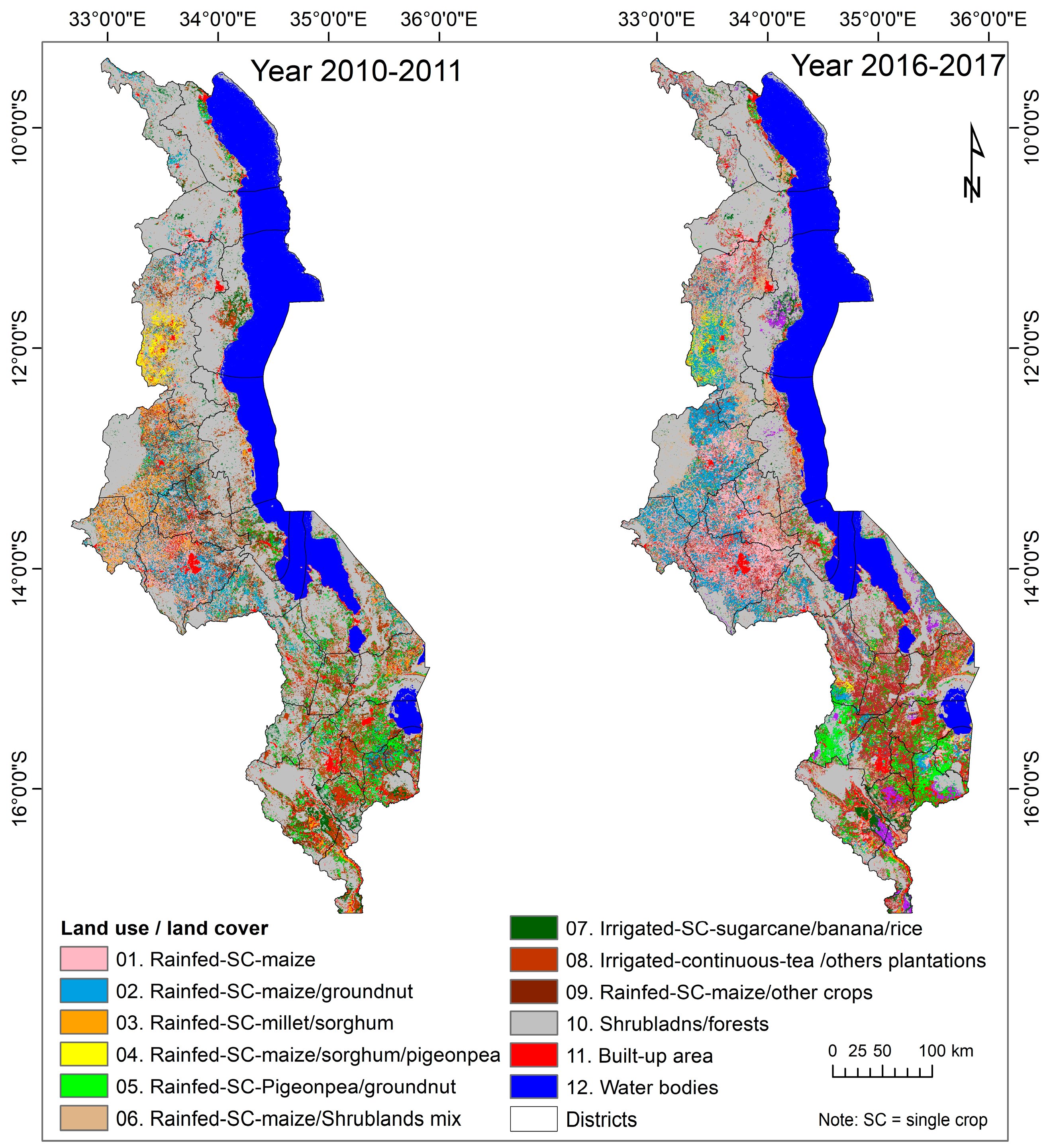In this study, we were able to surpass the atmospheric aberrations by using NDVI monthly MVCs [2]. The monthly MVC of NDVI time series classification successfully delineated cropping pattern in Malawi, as well as other land cover. Twelve classes have been identified from MODIS 250 m time series data (Figure 4) using SMTs. Almost 5.1 Mha of cropland was labelled as containing some portion of cultivation based on FPAs. However, when cropland area fractions were used, the actual (sub-pixel) area was 3.5 M ha for 2016–2017 (

Table 2. Cropland area for each class, providing an understanding of sub-pixel fractions for the 12 final classes in Malawi for the crop year 2016-2017.

LULC Fraction Categories	Full Pixel Areas (FPA) in ha	LULC Fraction (%)						Cropped Area
		Cropland	Trees	Grasses	Shrubs	Water	Other LULC
01. Rainfed-SC-maize	745,836	84	1	2	13	0	1	623,661
02. Rainfed-SC-maize/groundnut	874,807	75	1	0	20	0	4	654,311
03. Rainfed-SC-millet/sorghum/maize	98,302	63	0	3	33	0	1	62,258
04. Rainfed-SC-maize/sorghum/pigeonpea	103,757	95	2	0	2	0	1	98,829
05. Rainfed-SC-pigeonpea/groundnut/sorghum	472,419	85	2	0	11	0	2	402,029
06. Rainfed-SC-maize/shrub lands mix	786,944	69	1	0	29	1	1	542,429
07. Irrigated-SC-sugarcane/banana/rice	207,942	45	1	0	53	0	1	93,574
08. Irrigated-continuous-tea/other plantations	153,146	99	1	0	0	0	0	151,615
09. Rainfed-SC-maize/other crops	1,713,859	52	1	0	29	0	1	891,207
10. Scrublands/forests	4,044,605	NA	NA	NA	NA	NA	NA
11. Built-up area	335,354	NA	NA	NA	NA	NA	NA
12. Water bodies	2,300,270	NA	NA	NA	NA	NA	NA
Total cropped area								3,519,911

and

Table 3. Cropland area for each class, providing an understanding of sub-pixel fractions for the five important crops in Malawi for the crop year 2010–2011.

LULC#	Ground Data Sample Size	Cropped Area [49] (000ha)	Crop Fractions (%)					Crop Area (‘000 ha)
			Maize	Groundnut	Pigeonpea	Sorghum	Millet	Maize	Groundnut	Pigeonpea	Sorghum	Millet
01. Rainfed-SC-maize	19	301	0.8	0.2	0.0	0.0	0.0	253	32	0	0	0
02. Rainfed-SC-maize/groundnut	14	338	1.0	0.5	0.1	0.2	0.0	338	169	34	68	0
03. Rainfed-SC-millet/sorghum/maize	7	207	0.3	0.0	0.0	0.5	0.3	69	0	0	103	69
04. Rainfed-SC-maize/sorghum/pigeonpea	5	52	1.0	0.0	0.0	0.4	0.0	52	0	0	21	0
05. Rainfed-SC-pigeonpea/groundnut/sorghum	7	310	0.1	0.6	0.9	0.1	0.0	44	133	266	44	0
06. Rainfed-SC-maize/shrub lands mix	7	416	1.0	0.0	0.0	0.0	0.0	416	0	0	0	0
07. Irrigated-SC-sugarcane/banana/rice	2	202	0.0	0.0	0.0	0.0	0.0	0	0	0	0	0
08. Irrigated-continuous-tea/others plantations	7	112	0.8	0.0	0.0	0.0	0.0	0	0	0	0	0
09. Other crops	28	1138	0.4	0.0	0.0	0.0	0.0	566	0	0	0	0
Total area (ha)								1740	334	300	236	69

). The final class name was given based on the predominance of a specific land use (e.g., 02. Rainfed-SC-maize/groundnut) (Figure 4). Each class has several LULC types (see Table 3 and

Table 4. Cropland area for each class, providing an understanding of sub-pixel fractions for the 12 final classes in Malawi for the crop year 2010–2011.

LULC Fraction Categories	FPA (ha)	LULC Fraction (%)						Cropped Area
		Cropland	Trees	Grasses	Shrubs	Water	Other LULC
01. Rainfed-SC-maize	328,462	92	1	2	4	0	2	300,975
02. Rainfed-SC-maize/groundnut	493,539	69	1	0	29	1	1	338,427
03. Rainfed-SC-millet/sorghum/maize	245,723	84	2	0	13	0	1	206,758
04. Rainfed-SC-maize/sorghum/pigeonpea	679,22	77	1	2	19	0	0	524,36
05. Rainfed-SC-pigeonpea/groundnut/sorghum	365,132	85	2	0	1	0	12	310,362
06. Rainfed-SC-maize/shrub lands mix	483,984	86	1	0	13	0	0	416,226
07. Irrigated-SC-sugarcane/banana/rice	213,631	95	5	0	0	0	1	201,881
08. Irrigated-continuous-tea/other plantations	165,671	68	2	0	30	0	0	112,183
09. Rainfed-SC-maize/other crops	1,423,119	80	1	0	26	0	4	1,138,495
10. Scrublands/forests	5,414,178	NA	NA	NA	NA	NA	NA
11. Built-up area	330,464	NA	NA	NA	NA	NA	NA
12. Water bodies	2,304,482	NA	NA	NA	NA	NA	NA
Total cropped area								3,077,744

). For example, class 01 was described as Rainfed-SC-maize. Within this class, there were various other LULC, such as 1% trees, 2% grass, 4% shrubs and 2% other LULC (weeds, rocks, and built-up lands) and cultivable area (92%). In these cultivable areas, maize was the predominant crop, whereas groundnut was the next most dominant crop (

Table 5. Cropland area for each class, providing an understanding of sub-pixel fractions for the five important crops in Malawi for the crop year 2016–2017.

LULC#	Ground Data Sample Size	Cropped Area [49] (000ha)	Crop Fractions (%)					Crop Area (‘000 ha)
			Maize	Groundnut	Pigeonpea	Sorghum	Millet	Maize	Groundnut	Pigeonpea	Sorghum	Millet
01. Rainfed-SC-maize	21	624	0.7	0.1	0.0	0.0	0.0	445	89	0	0	0
02. Rainfed-SC-maize/groundnut	40	654	0.7	0.1	0.1	0.0	0.0	458	65	33	0	0
03. Rainfed-SC-millet/sorghum/maize	3	62	0.3	0.0	0.0	0.3	0.3	21	0	0	21	21
04. Rainfed-SC-maize/sorghum/pigeonpea	4	99	0.8	0.0	0.3	0.1	0.0	74	0	25	12	0
05. Rainfed-SC-pigeonpea/groundnut or sorghum	6	402	0.6	0.3	0.7	0.1	0.0	223	134	268	45	0
06. Rainfed-SC-maize/shrub lands mix (30%)	14	542	0.4	0.0	0.0	0.0	0.1	232	0	0	0	39
07. Irrigated-SC-sugarcane/banana/rice	2	94	0.0	0.0	0.0	0.0	0.0	0	0	0	0	0
08. Irrigated-continuous-tea/other plantations	25	152	0.0	0.0	0.0	0.0	0.0	0	0	0	0	0
09. Other crops	18	891	0.6	0.1	0.1	0.1	0.0	545	99	50	50	0
Total area (ha)								1999	388	375	127	59

).

Using the same approach, total cropland area was estimated to be 3,519,911 ha, which included irrigation by lake (245,188 ha). In Figure 4b, it was observed that maize was predominantly grown throughout Malawi (Figure 4b). Pigeonpea and sorghum were grown in the southern regions (Mualanje, Mwanza, Zomba and Chikwawa). Sorghum and millet are grown in southern Malawi, in the dry land areas of Nsanje, and Plantations (class 08) were located in Thyolo and Chickwawa.

4.2. Spatio-Temporal Changes in Pigeonpea and Groundnut

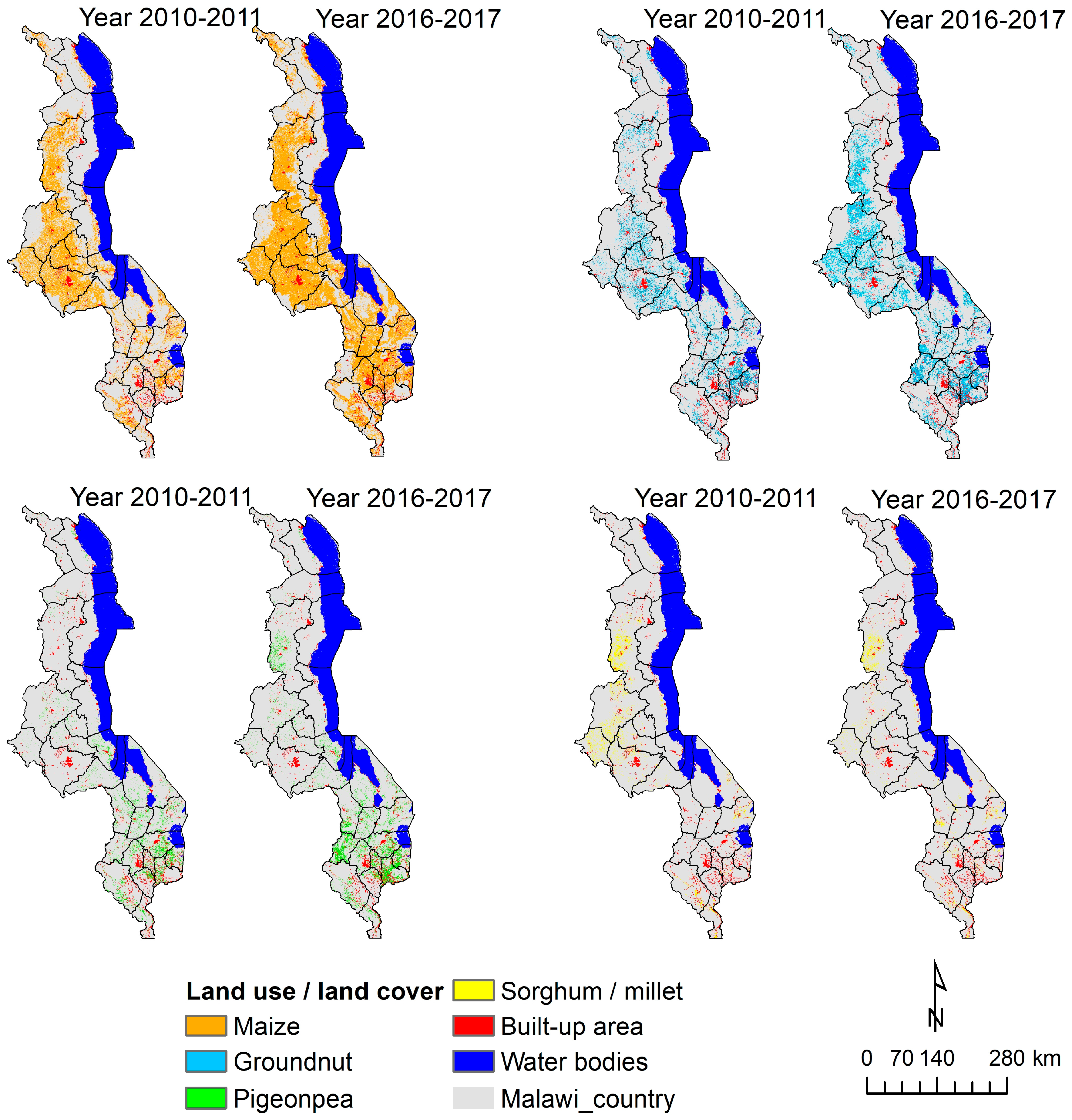
The areas planted with maize, pigeonpea, groundnut, and sorghum/millet for each district in Malawi for 2010–2011 and 2016–2017 are presented in Figure 5 and

Table 6. District-wise cropped areas (ha) extracted from MODIS-derived areas for 2010–2011 and 2016–2017.

District	Maize (ha)		Groundnut (ha)		Pigeonpea (ha)		Sorghum (ha)		Millet (ha)
	2010–2011	2016–2017	2010–2011	2016–2017	2010–2011	2016–2017	2010–2011	2016–2017	2010–2011	2016–2017
Balaka	36,147	62,176	8920	14,657	14,749	16,302	3206	6188	86	194
Blantyre	26,334	51,536	9001	11,517	14,287	14,760	3177	4706	30	859
Chikwawa	51,086	72,726	10,793	16,758	20,253	19,778	9429	7395	3917	2911
Chiradzulu	15,780	23,975	4053	7697	7045	11,975	1496	2851	71	307
Chitipa	33,383	35,558	7981	5011	3420	3415	3217	1552	164	1685
Dedza	92,478	93,772	23,639	16,983	12,629	11,752	10,570	3579	1458	1627
Dowa	64,815	119,662	12,240	21,507	4280	7033	7656	2727	2482	1716
Karonga	19,081	21,943	4162	3550	4567	4167	3252	2036	1165	1979
Kasungu	201,318	225,790	25,034	35,524	11,517	17,554	31,075	6373	15,105	6639
Lilongwe	222,150	202,463	41,563	34,505	6826	7877	24,822	4989	7781	2778
Machinga	55,968	72,463	12,218	16,166	19,376	19,383	9951	8682	3818	3770
Mangochi	81,277	106,251	20,156	22,121	24,298	24,791	10,093	8527	2075	2271
Mchinji	113,386	103,420	12,033	16,605	4280	7269	20,919	3973	11,824	3095
Mulanje	28,637	53,331	13,851	20,835	19,486	35,606	5575	6774	444	173
Mwanza	16,801	53,294	5099	23,806	8718	43,926	1766	8254	8	4
Mzimba	259,727	261,862	21,671	26,538	4695	24,010	40,789	14,731	8678	15,333
Nkhata Bay	5829	7373	41	676	40	350	151	375	90	664
Nkhotakota	38,780	44,573	1920	4518	1772	3052	3106	2790	1610	4428
Nsanje	16,684	24,096	3286	5043	6413	6324	5351	3553	2848	2189
Ntcheu	44,782	80,605	13,015	16,538	17,692	19,891	4754	6757	96	728
Ntchisi	48,079	54,827	8114	9477	4065	3775	3677	1200	530	1247
Phalombe	30,102	45,433	14,545	13,290	21,196	17,713	6232	3959	748	408
Rumphi	26,961	24,657	6382	4245	3125	2646	1990	1048	135	972
Salima	39,693	49,111	10,143	11,687	14,215	12,883	3869	3733	186	835
Thyolo	8888	28,562	5346	6633	10,603	9550	1788	2619	2	1328
Zomba	47,404	74,148	18,883	20,696	31,722	28,035	7483	7603	665	1157
Total	1,625,569	1,993,605	314,088	386,582	291,268	373,819	225,391	126,973	66,014	59,295

. Maize was the major crop grown across Malawi (Figure 5) with an increased area in 2016–2017 compared to 2010–2011, mainly in the southern districts and a slight increase in other districts. Pigeonpea was mainly grown in districts like Mzimba, Salima, Balaka, Mwanza, Zomba, Phalmobe, Mulanje, Machinga, Blantyre, and Chikwawa. There was a high increase in pigeonpea area during 2016–2017 mainly in Mwanza and Mzimba compared to the 2010–2011. Table 6 shows the district-wise cropped areas for the crop years 2010–2011 and 2016–2017. Groundnut was mainly grown in almost all the districts. There was a high increase mainly in Mzimba, Kasungu, Mchinji, Liongwe, and Mwanze and a less increase in some parts of other districts in 2016-2017 compared to 2010-2011. Sorghum/millet was grown in districts like Mzimba, Kasungu, and Mchinji and sparsely in other parts. A decrease in sorghum/millet area during 2016–2017 was observed mainly in Kasungu, Mchinji, and Lilongwe compared to 2010–2011. Majority of sorghum/millet was replaced by maize/groundnut. In some parts of Mzimba district, maize/sorghum/pigeonpea was replaced with pigeonpea/groundnut. Considering the distribution of cropland area under each class, a total of about 442,167 ha was added to cropped area in 2016–2017.

A close look at the distribution of agricultural area from 2010–2011 to 2016–2017 (Figure 5) shows that the LULC fraction (%) increased mainly in the following classes: Rainfed—SC-maize/sorghum/pigeonpea from 77% to 95 percent, Rainfed-SC-maize/groundnut from 69% to 75%, and Irrigated-continuous-tea/others plantations from 68% to 99%. It decreased mainly in classes like Rainfed-SC-maize from 92% to 84%, Rainfed-SC-millet/sorghum/maize from 84% to 63%, Rainfed-SC-maize/shrub lands mix from 86% to 69%, Irrigated-SC-sugarcane/banana/rice from 95% to 45%, and Rainfed-SC-maize/other crops from 80% to 52%. However, there was an increase in cropped area [49] mainly in classes like Rainfed-SC-maize from 300,975 ha to 623,661 ha, Rainfed-SC-maize/groundnut from 338,427 ha to 654,311 ha, Rainfed-SC-maize/sorghum/pigeonpea from 52,43 6ha to 98,829 ha, Rainfed-SC-pigeonpea/groundnut/sorghum from 310,362 ha to 402,029 ha, Rainfed-SC-maize/shrub lands mix from 416,226 ha to 542,429 ha, and Irrigated-continuous-tea/others plantations from 112,183 ha to 151,615 ha. There was a decrease in cropped area mainly in classes like Rainfed-SC-millet/sorghum/maize from 206,758 ha to 62,258 ha, Irrigated-SC-sugarcane/banana/rice from 201,881 ha to 92,574 ha, and Rainfed-SC-maize/other crops from 1,138,495 ha to 891,207 ha. Spatial variations are shown in Figure 5.

Considering the crop fractions (%) in LULC from 2010–2011 to 2016–2017 (Table 3 and Table 5), there was an increase of pigeonpea in Rainfed-SC-maize/sorghum/pigeonpea from 0.0% to 0.3%, and other crops from 0.0% to 0.1%. For maize, there was a slight decrease in crop fractions, i.e., Rainfed-SC-maize from 0.8% to 0.7%, Rainfed-SC-maize/groundnut from 1.0% to 0.7%, Rainfed-SC-maize/sorghum/pigeonpea from 1.0% to 0.8%, and Rainfed-SC-maize/shrub lands mix from 1.0% to 0.4%. For groundnut, there was also a decrease in crop fractions i.e., Rainfed-SC-maize from 0.2% to 0.1%, Rainfed-SC-maize/groundnut from 0.5% to 0.1%, and Rainfed-SC-pigeonpea/groundnut/sorghum from 0.6% to 0.3%. For sorghum, there was a decrease in crop fractions, i.e., Rainfed-SC-maize/groundnut from 0.2% to 0.0%, Rainfed-SC-millet/sorghum/maize from 0.5% to 0.3%, and Rainfed-SC-maize/sorghum/pigeonpea from 0.4% to 0.1%. There were no changes in the crop fractions for pearl millet.

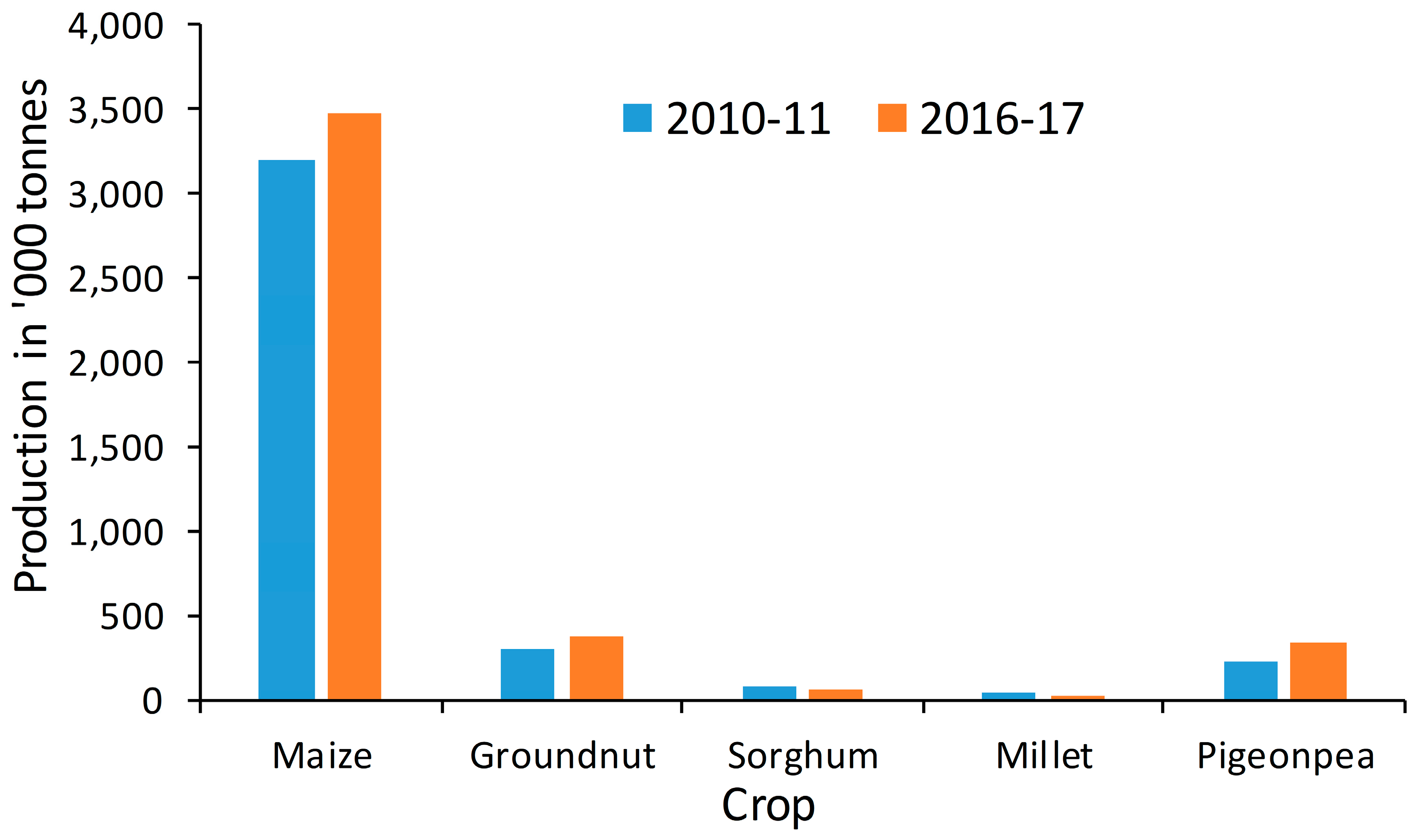
The changes in five major crops from 2010–2011 to 2016–2017 revealed that there was an increase in crop area under maize from 1,740,000 ha to 1,999,000 ha, Groundnut area increased from 334,000 ha to 388,000 ha, pigeonpea from 300,000 ha to 375,000 ha, a considerable decrease in sorghum area from 236,000 ha to 127,000 ha, and millet area from 69,000 ha to 59,000 ha. The area increase in pigeonpea was attributed to the rising demand for export to South Asia driven by the increasing population and income in South Asia. Mwaiwathu alimi (ICEAP 00557) is a climate-resilient medium-duration variety released in Malawi. This variety also has a trait preferred by traders, i.e., the plum cream-colored grain. This variety has therefore provided an opportunity to expand pigeonpea area into the livestock-dominant central region and short growing season in northern Malawi. During the same period, several donors supported legumes research and development efforts, including seed systems, which gave a fillip to the expansion of both of the legumes. Furthermore, improved versions of Mwaiathu alimi were recently registered, namely, Chitedze Pigeonpea 1 (ICEAP 01514/15) and Chitedze Pigeonpea 2 (ICEAP 01485/3), which are expected to contribute to further expansion of pigeonpea in Malawi.

4.3. Accuracy Assessment

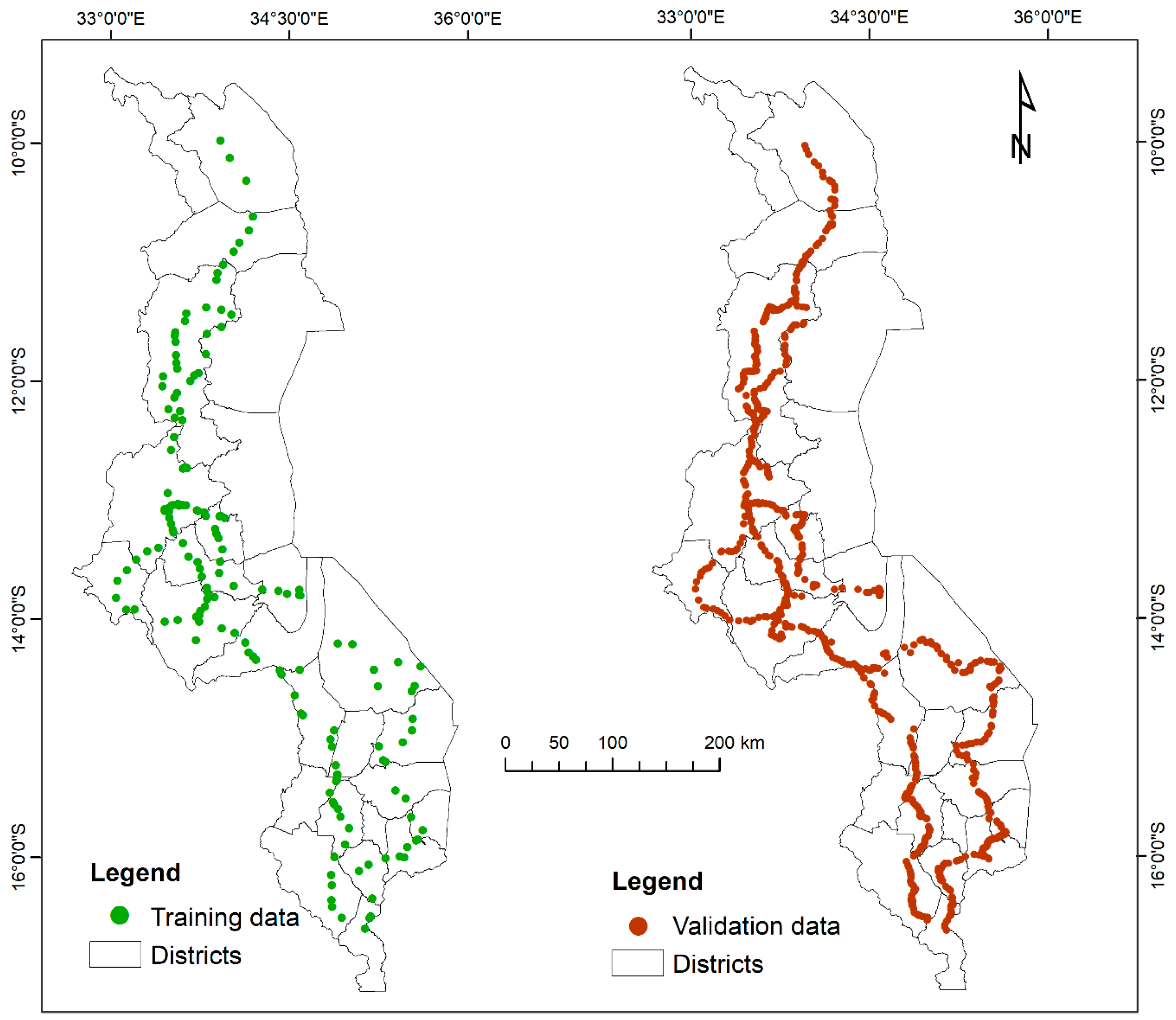
Accuracy assessment was carried out using 614 ground samples (Figure 2). An error matrix (

Table 7. Accuracy assessment using ground survey data using error matrix method for the year 2016-2017.

Classified Data	Reference Data (Ground Survey Data)												Classified Totals	Number Correct	Producer Accuracy (%)	Users Accuracy (%)	Kappa
	CL_1	CL_2	CL_3	CL_4	CL_5	CL_6	CL_7	CL_8	CL_9	CL_10	CL_11	CL_12
CL_1	96	0	1	7	1	0	0	0	0	4	0	0	109	96	75	88	0.8
CL_2	18	99	1	3	0	0	0	0	2	12	0	0	135	99	97	73	0.7
CL_3	1	0	5	0	0	0	0	0	0	0	0	0	6	5	63	83	0.8
CL_4	0	0	0	8	0	0	0	0	0	4	0	0	12	8	40	67	0.7
CL_5	5	1	0	1	34	0	0	0	6	2	1	0	50	34	56	68	0.6
CL_6	4	1	0	0	0	48	0	0	0	8	0	0	61	48	100	79	0.8
CL_7	0	1	0	0	2	0	16	3	0	1	0	0	23	16	100	70	0.7
CL_8	1	0	0	0	0	0	0	10	0	0	0	0	11	10	77	91	0.9
CL_9	3	0	1	1	24	0	0	0	86	4	0	0	119	86	91	72	0.7
CL_10	0	0	0	0	0	0	0	0	0	70	0	0	70	70	67	100	1.0
CL_11	0	0	0	0	0	0	0	0	0	0	15	0	15	15	94	100	1.0
CL_12	0	0	0	0	0	0	0	0	0	0	0	3	3	3	100	100	1.0
Column Total	128	102	8	20	61	48	16	13	94	105	16	3	614	614

Overall Classification Accuracy = 79.80%; Overall Kappa Statistics = 0.7648.

) showing the agreement (and disagreement) between the classified map and the ground points was prepared. Two measures of accuracy—Overall accuracy and Kappa coefficient—were computed. Though overall accuracy gives an estimate of the overall correctness of the map as a whole, it cannot provide a measure for the accuracy of individual LULC classes. Since the classes occupy different extents on the map, the overall accuracy is high when the class occupying a large area is correctly classified, in spite of the other classes being wrongly interpreted. This is corrected by the Kappa coefficient, which takes into account the user’s and producer’s accuracies of each class. It is calculated using Equation (4).

$$\kappa =\frac{N{\sum }_{i=1}^r{x}_{ii} - {\sum }_{i=1}^r\left(x_{i+ } \times x_{+i }\right)}{N^2 -{\sum }_{i=1}^r\left(x_{i+ } \times x_{+i }\right)}$$

(4)

where N is the total number of sites in the error matrix, r is the number of rows in the error matrix, x_ii is the number in row i and column i, x_+i is the total for row i, and x_i+ is the total for column i [50].

The overall classification accuracy for the map of the year 2016–2017 was 79.8% and the overall Kappa coefficient was 0.76. Majority classes showed producer’s accuracy and user’s accuracy of more than 70%. Some classes with mixed crops, class 4 for example, had low accuracy level, 40% producer’s accuracy and 67% user’s accuracy because there was a mix of pigeonpea, maize and sorghum. Ground data collected did not coincide with the assigned class (average land holding size is 1.2 ha) as the imagery used was of coarse resolution. Classes with low accuracies can be improved by taking the following measures: (a) collecting extensive ground sample data; (b) undertaking regional analysis; (c) taking land related information like soils, slope and elevation into consideration in the analysis; (d) taking care while collecting mixed crop ground sample data; (e) resolving mixed classes; and (f) using higher resolution time series data like Landsat 30 m. Spectral matching techniques have limitations where there are few ideal spectra signatures. This occurs when particular classes have very few ground survey points because the areas are located in interior areas with no road access [29,30]. Another limitation is collecting ground survey data, which is time consuming and expensive. Time can be saved and data can be less error-prone when ground data is captured using mobile applications (crops, global croplands, etc.). Ground survey data were also used to address the problem of coarse resolution (MODIS) when the coarser resolution is used to map and characterize ground sample that are smaller than pixel areas where multiple crops are present in the same pixel [29,30]. It is important to note that lower accuracy is also due to coarse spatial resolution of MODIS (each pixel is 250 m on each side and larger than many agricultural fields in the study area). Many pixels can have multiple land use/land cover types because of small holdings. High resolution imagery such as sentinel-2 with 5-day intervals in the same geometry and, multiband synthetic aperture radar (SAR) with 12-day interval data offers new possibilities for accurate mapping and avoiding these gaps [51].

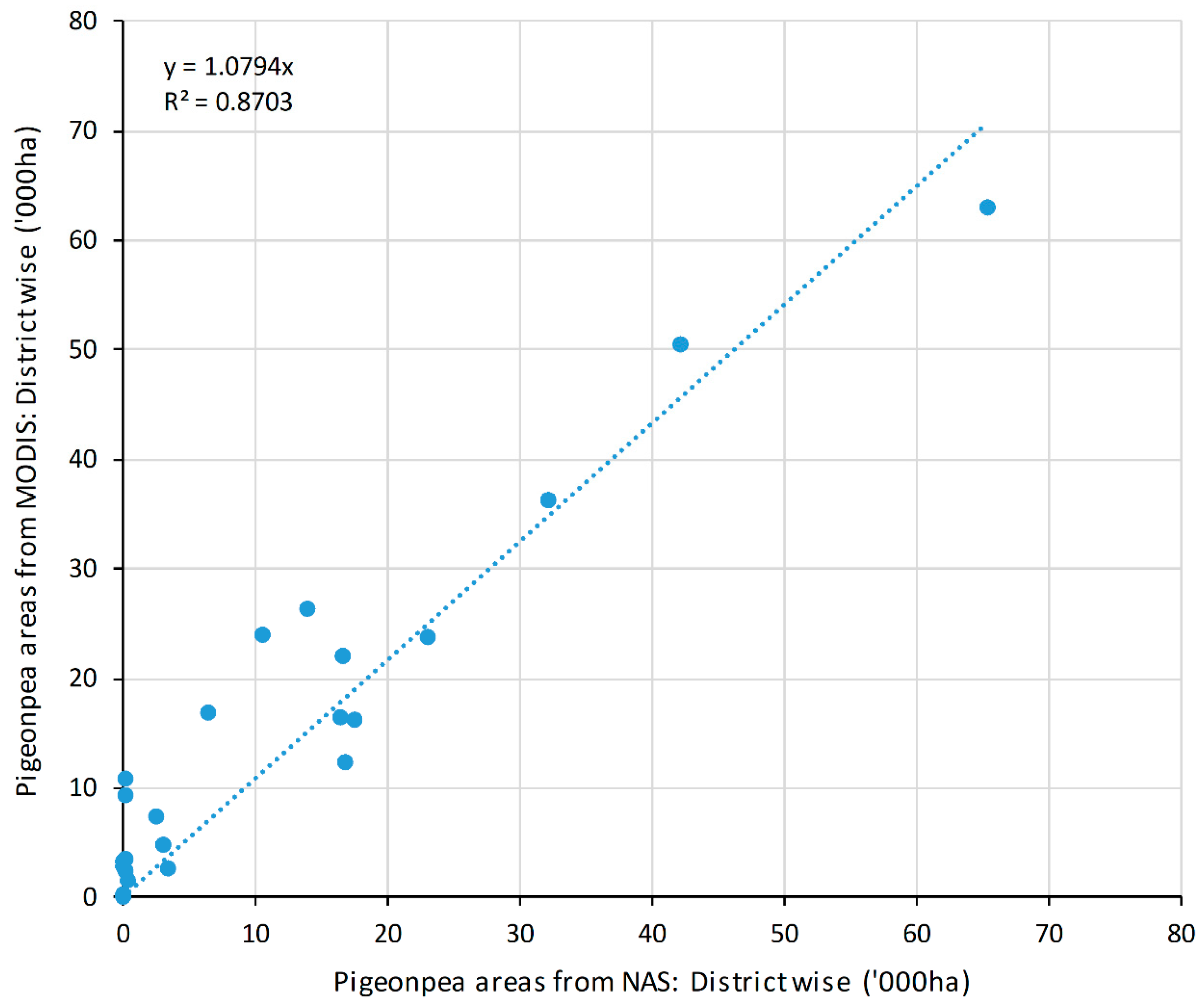
4.4. Comparison with Sub-National Statistics

Pigeonpea is one of the major crops in Malawi and its net sown area is increasing rapidly. The district-wise areas derived from our study (MODIS) for the year 2016 were plotted with national agricultural statistics (NAS) [40], and Pearson’s coefficient of correlation was computed. There was a significant and positive linear correlation with an R² value of 0.870 and the slope coefficient of 1.08 (Figure 6).

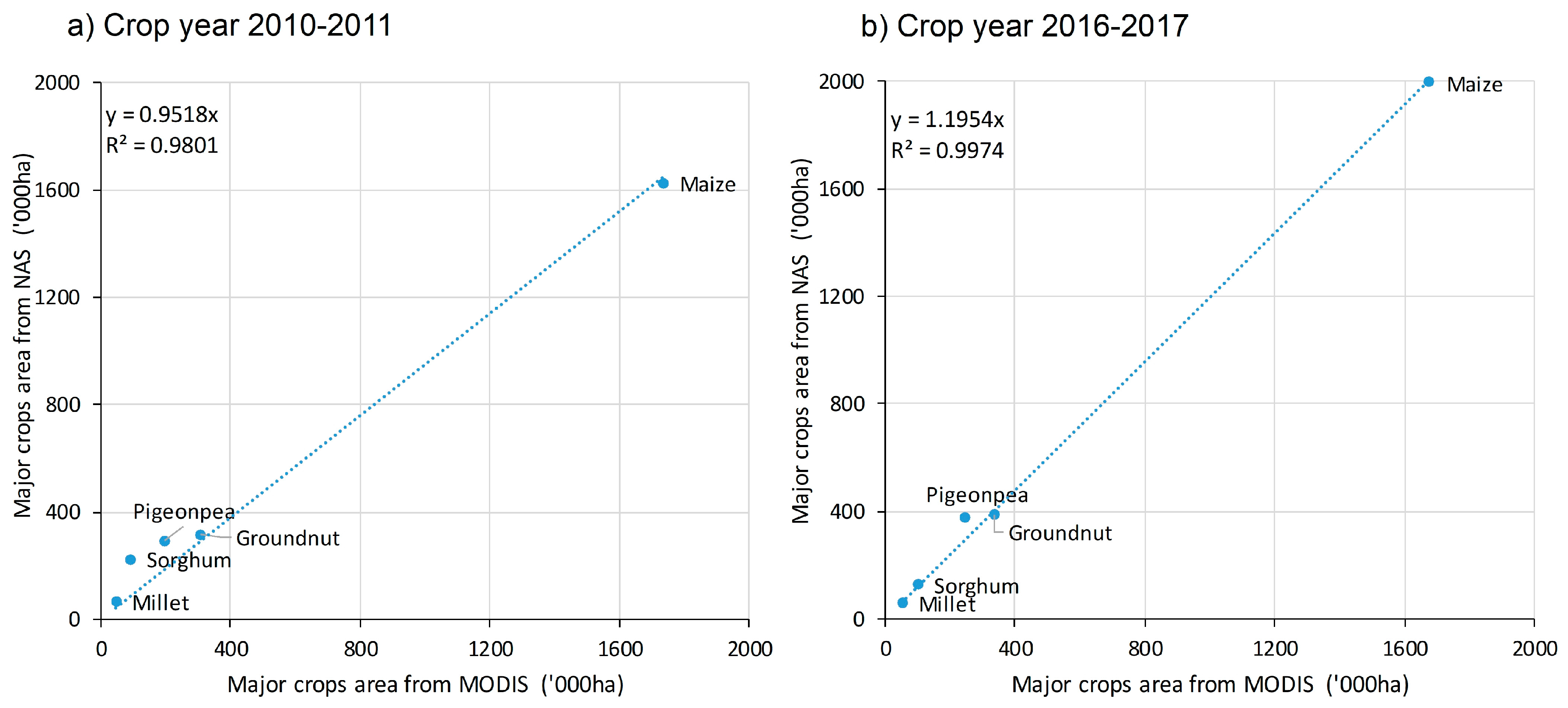
The areas of cultivation of Malawi’s five important crops (maize, pigeonpea, groundnut, sorghum, and millet) taken from the NAS were plotted against the data obtained from the MODIS imagery, and a significant and positive correlation was seen with R² values of 0.98 and 0.99 for the crop years 2010–2011 and 2016–2017, respectively (Figure 7). For 2010–2011, there was a major difference in maize, pigeonpea, and sorghum due to mixed cropping and a slight difference among other crops. For 2016–2017, there were major differences in the maize and pigeonpea because with the growth in agricultural area in Malawi (Figure 8), the cultivation of mixed crops had been increasing along with the maize area.

A comparison of cultivated areas in 2010–2011 and 2016–2017 showed that for 2016–2017, there was an appreciable increase in pigeonpea cultivation in many districts of Malawi along with some other crops (Table 6). Data from some districts showed large difference due to intermixing of various classes. The coarse resolution of the image data may have caused the mixing of classes.

4.5. Impact of ICRISAT Technologies on the Extensification and Productivity Enhancement of Groundnut and Pigeonpea

Groundnut and pigeonpea are two important dryland legumes that earn large export revenue and provide high returns to smallholder farmers of Malawi. The adoption of new technologies in crops developed by DARS under the auspices of ICRISAT was initially slow due to low awareness, the absence of organized seed systems and a biased government extension towards maize, the staple cereal crop. ICRISAT’s groundnut breeding hub not only provided improved groundnut varieties during its three-decade presence in Malawi but also introduced its improved pigeonpea technologies as a strategy to improve the nutritional security by adding plant protein to the food basket. The ICRISAT-led Tropical Legumes II project, which ended in 2015 was a major contributor to development and delivery of the improved groundnut and pigeonpea varieties. After the government realized the importance of farmer participatory varietal selection and breeding in the late 90′s, farmers were enabled to select desirable traits suited to local production systems and market demand, leading to the adoption of the new varieties (

Table 8. Pigeonpea varieties released in Malawi and their characteristics.

Variety	Pedigree	Year	Special Varietal Attributes	Recommended Agro Ecologies	Yield (kg/ha)
Sauma	ICP 9145	1987	Long duration, fusarium wilt resistant	High altitude area	1500
Kachangu	ICEAP 00040	2000	Long duration, large seeded	High altitude area	2000
ICPL 87105	ICPL 87105	2003	Short duration, multiple cropping	Low to medium altitude areas	2000
ICPL 93027	ICPL 93,027	2003	Short duration, multiple cropping	Low to medium altitude areas	2000
Mwaiwathualimi	ICEAP 00557	2009	Medium duration	Low to medium altitude areas	2500
Chitedze Pigeonpea 1	ICEAP 01514/15	2011	Medium duration, high yielding	Low to medium altitude areas	2500
Chitedze Pigeonpea 2	ICEAP 01485/3	2014	Medium duration, high yielding	Low to medium altitude areas	2500

Source: Tropical Legumes II project report [52].

) [52].

The major areas growing of pigeonpea are Mwanza and Mulanje in the southern region. This region accounts for 92% of the total pigeonpea area contributing up to about 20% of farmers’ incomes. Intercropping with maize is a widely adopted practice. In the northern districts of Karonga and Chitipa and in the central districts of Slima, Kasungu, Lilongwe and Mchingji, there is great potential for medium duration varieties. ICRISAT’s contribution of medium duration pigeopnpea to these new areas has not only helped fulfil pigeonpea demand in Malawi but has also contributed to the economic recovery program of its government [52].

4.6. Economic Factors

Since 2010–2011, pigeonpea productivity and production of pigeonpea have been increasing with the release and adoption of ICRISAT-bred medium-duration varieties, farmers’ access to quality seed through a revolving seed scheme, and the government’s support to inputs, including seeds. During the study period, it recorded positive trends in both productivity (34.6% increase) and production (68.7%). About 35% of the produce is sold through formal markets, with most sales going to the export market [53]. It is exported either as whole grain or as processed grain, i.e., split decorticated grain known in India as dhal. Whole grain is exported to India, whereas the dhal is mainly exported to the South Asian people in Europe (mainly the UK) and the USA. About 10% of the dhal stays in Malawi for domestic consumption [54]. Malawi is the fourth largest exporter of pigeonpea to India, contributing to about 35% of the country’s requirement. While pigeonpea prices in India peak in November–December, its harvesting between July and September in Malawi and export coincide with India’s period of relative shortage and high prices [53].

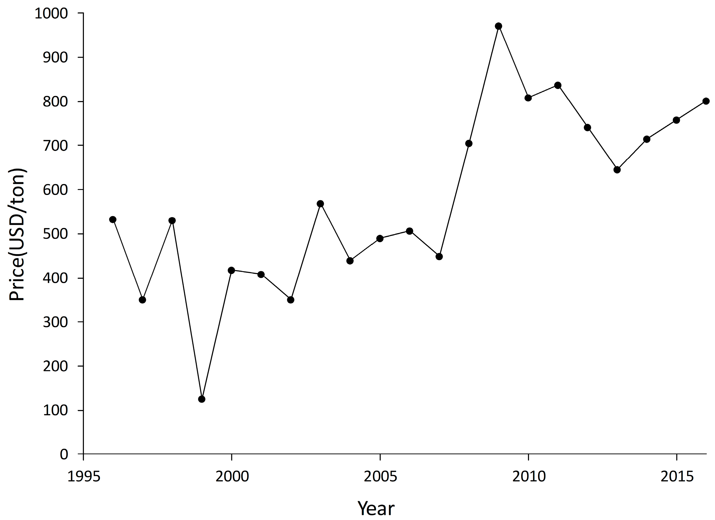
Producer prices of pigeonpea in Malawi show a positive trend with year-to-year variations (Figure 9). A poor harvest in India increases the demand for imports, resulting in high prices that encourage Malawian growers to increase the area planted with the crop. While there are remarkable variations depending on weather conditions in India, there is generally an increasing trend due to rising population and income levels among consumers in India, which has been driving the expansion of pigeonpea area in Malawi.

Malawi’s pigeonpea export is handicapped by its landlocked location, resulting in high transportation costs. Freight charges from Malawi are USD 130 per ton, compared to USD 50 per ton for Mozambique, for instance [9]. Nonetheless, Malawian producers have managed to compete in the world market for three reasons, the government subsidizes exports by giving a 25% rebate on freight charges from taxable profits; its pigeonpea is considered to be of good quality and a recognizable brand and exporters can earn a premium price for white pigeonpea grain, while red/speckled grain reduces the price by 5–10%. There is a price difference of USD 150 per ton between the price of Burmese lemon pigeonpea and Malawian white pigeonpea [9].

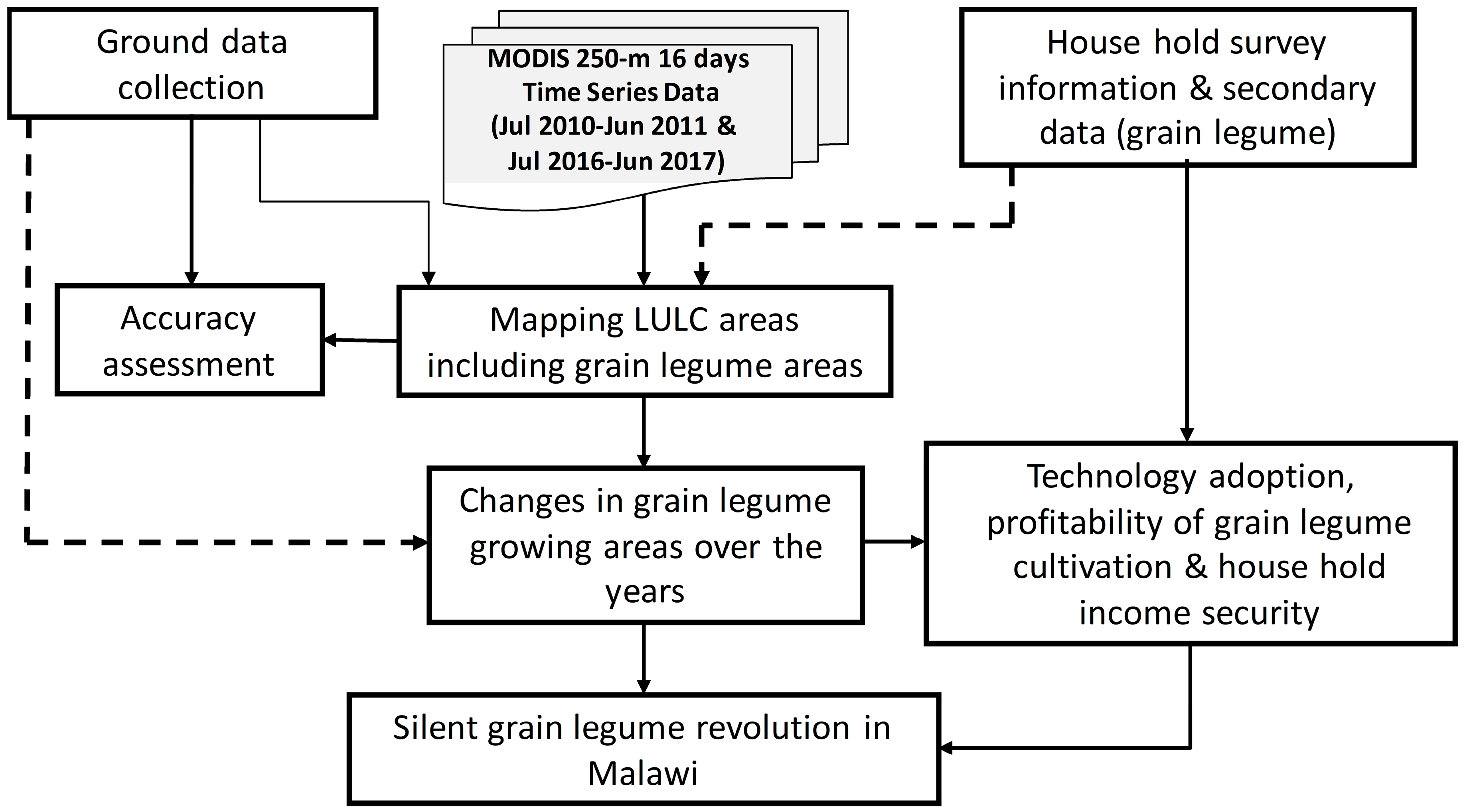
4.7. Income, Livelihood Security and Profitability of Grain Legume Cultivation in Malawi

A number of studies have been conducted in Malawi to assess measures adopted by smallholder farmers to enhance incomes and livelihood security at the household level [55,56]. These measures include both on-farm and off-farm activities. On-farm activities are these that bring income to the household through the production of crops and keeping livestock on one’s own farm or garden. Off-farm activities are done outside one’s farm, e.g., obtaining income from temporary employment and operating a small business enterprise to supplement income from on-farm activities. Most smallholder farmers in Malawi largely depend on tobacco, cereal and legume cultivation for sustenance, incomes and livelihood security at the household level. The government has also been encouraging farmers to diversify crop production in order to avert the adverse impacts of climate variability and climate change as well as to tackle malnutrition arising from maize-dominant diets. Thus, in addition to growing maize, farmers are encouraged to grow drought-tolerant and nutritious crops such as potato, cassava, sorghum, millet and legumes. Although production of sorghum and millet has declined, production of legume crops has dramatically increased (e.g., Table 6) owing to the market opportunities.

Grain legumes continue to play an important role in human nutrition as a source of protein, vitamins and minerals [57,58]. Legumes improve soil fertility by fixing nitrogen in the atmosphere there by playing a dual role. The discourse in this section focuses on profitability of grain legumes cultivation in Malawi with regard to their respective gross margins.

Farmers in Malawi are interested in growing legume crops for consumption as well as for sale in the market. The produce is not only marketable for profit, but there is also an awareness about the need for demand-driven technologies. This has led to many transformations in society, including gender equity. The area, yield and production of common bean, groundnut and soybean fluctuated between 1990 and 2012, showing an upward trend [59]. The implementation of government subsidies, market access, demand for local consumption, availability of suitable traits in improved seeds and finally the attractive price have all contributed to increasing the area and production of these legumes in Malawi.

5. Conclusions

Pigeonpea and groundnut crops have made inroads into the cereal dominated farming systems of Malawi, improving soil fertility, human nutrition, productivity and income earning opportunities. This study provided a comprehensive assessment of cropping patterns and major cropland changes in Malawi at national and sub-national levels using remotely sensed data. Spatio-temporal cropland changes are useful for monitoring, supporting diffusion and value addition of cash crops like pigeonpea. For crop breeders, tracking the spread of released varieties and genetic gain are key metrics. Results show that the area planted with pigeonpea increased by 75,000 ha from 2010–2011 to 2016–2017, maize by 259,000 ha and groundnut by 54,000 ha. On the other hand, sorghum and millet areas decreased by 109,000 ha and 10,000 ha, respectively, during the same period. By mapping information on the cropping patterns of major crops using satellite imagery at the national and sub-national level, suitable locations can be identified to demonstrate and scale up best-bet management practices, and to promote better varieties of crops.

References

1. FAO. National Investment Profile. Water for Agriculture and Energy: Malawi. 2015. Available online: www.Fao.Org/fileadmin/user_upload/agwa/docs/nip_malawi_final.Pdf (accessed on 12 May 2019).
2. Bank, W. Malawi Agricultural Sector Memorandum: Strategy Options in the 1990s; World Bank: Washington, DC, USA, 1995. [Google Scholar]
3. FAO. Fao/wfp Crop and Food Supply Assessment Mission to Malawi. 2018. Available online: http://www.Fao.Org/docrep/005/y9667e/y9667e00.Htm (accessed on 23 September 2018).
4. Tsusaka, T.W.; Msere, H.W.; Siambi, M.; Mazvimavi, K.; Okori, P. Evolution and impacts of groundnut research and development in malawi: An ex-post analysis. Afr. J. Agric. Res. 2016, 11, 139–158. [Google Scholar]
5. Giertz, A.; Caballero, J.; Galperin, D.; Makoka, D.; Olson, J.; German, G. Malawi Agricultural Sector Risk Assessment; Agriculture global practice technical assistance paper; World Bank: Washington, DC, USA, 2015; Available online: https://openknowledge.worldbank.org/handle/10986/23678 (accessed on 21 June 2019).
6. Smith, A.; Snapp, S.; Dimes, J.; Gwenambira, C.; Chikowo, R. Doubled-up legume rotations improve soil fertility and maintain productivity under variable conditions in maize-based cropping systems in Malawi. Agric. Syst. 2016, 145, 139–149. [Google Scholar] [CrossRef]
7. Ministry of Agriculture, Irrigation and Water Development (MoAIWD). Global Agriculture and Food Security Programme: Support to Malawi’s Agricultural Sector Wide Approach (Aswap): Proposal from Malawi Government; Agricultural Communication Branch: Lilongwe, Malawi, 2012.
8. FAOSTAT. United Nation’s Food and Agriculture Organization. Rome, Italy. 2018. Available online: http://www.fao.org/faostat/en/#data/pp (accessed on 11 May 2018).
9. Orr, A.; Amede, T.; Tsusaka, T.; Tiba, Z.; Dejen, A.; Deneke, T.T.; Phiri, A. Smallholder Risk Management Solutions (Srms) in Malawi and Ethiopia: Risk Management Scoping Study; Oxford Policy Management: Oxford, UK, 2017; p. 58. [Google Scholar]
10. Singh, A.K.; Singh, S.; Prakash, V.; Kumar, S.; Dwivedi, S. Pulses production in india: Present status, sent status, bottleneck and way forward. J. AgriSearch 2015, 2, 75–83. [Google Scholar]
11. Thenkabail, P.S.; Knox, J.W.; Ozdogan, M.; Gumma, M.K.; Congalton, R.G.; Wu, Z.; Milesi, C.; Finkral, A.; Marshall, M.; Mariotto, I. Assessing future risks to agricultural productivity, water resources and food security: How can remote sensing help? Photogramm. Eng. Remote Sens. 2012, 78, 773–782. [Google Scholar]
12. Thiruvengadachari, S.; Sakthivadivel, R. Satellite Remote Sensing for Assessment of Irrigation System Performance: A Case Study in India. Research Report 9; International Irrigation Management Institute: Colombo, Sri Lanka, 1997. [Google Scholar]
13. Lobell, D.B.; Asner, G.P.; Ortiz-Monasterio, J.I.; Benning, T.L. Remote sensing of regional crop production in the yaqui valley, mexico: Estimates and uncertainties. Agric. Ecosyst. Environ. 2003, 94, 205–220. [Google Scholar] [CrossRef]
14. Thenkabail, P.; Hanjra, M.; Dheeravath, V.; Gumma, M. A holistic view of global croplands and their water use for ensuring global food security in the 21st century through advanced remote sensing and non-remote sensing approaches. Remote Sens. 2010, 2, 211–261. [Google Scholar] [CrossRef]
15. Ayele, G.T.; Demessie, S.S.; Mengistu, K.T.; Tilahun, S.A.; Melesse, A.M. Multitemporal land use/land cover change detection for the batena watershed, rift valley lakes basin, Ethiopia. In Landscape Dynamics, Soils and Hydrological Processes in Varied Climates; Springer International Publishing: Cham, Switzerland, 2016; pp. 51–72. [Google Scholar]
16. Fu, P.; Weng, Q. A time series analysis of urbanization induced land use and land cover change and its impact on land surface temperature with landsat imagery. Remote Sens. Environ. 2016, 175, 205–214. [Google Scholar] [CrossRef]
17. Li, J.; Jiang, H.; Bai, Y.; Alatalo, J.M.; Li, X.; Jiang, H.; Liu, G.; Xu, J. Indicators for spatial–temporal comparisons of ecosystem service status between regions: A case study of the taihu river basin, China. Ecol. Indic. 2016, 60, 1008–1016. [Google Scholar] [CrossRef]
18. Xia, T.; Wu, W.; Zhou, Q.; Verburg, P.H.; Yu, Q.; Yang, P.; Ye, L. Model-based analysis of spatio-temporal changes in land use in northeast China. J. Geogr. Sci. 2016, 26, 171–187. [Google Scholar] [CrossRef]
19. Gaur, A.; Biggs, T.W.; Gumma, M.K.; Parthasaradhi, G.; Turral, H. Water scarcity effects on equitable water distribution and land use in a major irrigation project—Case study in India. J. Irrig. Drain. Eng. 2008, 134, 26–35. [Google Scholar] [CrossRef]
20. Biggs, T.W.; Gangadhara Rao, P.; Bharati, L. Mapping agricultural responses to water supply shocks in large irrigation systems, southern India. Agric. Water Manag. 2010, 97, 924–932. [Google Scholar] [CrossRef]
21. Gumma, M.K.; Andrew, N.; Thenkabail, P.S.; Amrendra, N.S. Mapping rice areas of south asia using modis multitemporal data. J. Appl. Remote Sens. 2011, 5, 053547. [Google Scholar] [CrossRef]
22. Xu, Y.; Yu, L.; Zhao, F.R.; Cai, X.; Zhao, J.; Lu, H.; Gong, P. Tracking annual cropland changes from 1984 to 2016 using time-series landsat images with a change-detection and post-classification approach: Experiments from three sites in africa. Remote Sens. Environ. 2018, 218, 13–31. [Google Scholar] [CrossRef]
23. Liu, F.; Zhang, Z.; Zhao, X.; Wang, X.; Zuo, L.; Wen, Q.; Yi, L.; Xu, J.; Hu, S.; Liu, B. Chinese cropland losses due to urban expansion in the past four decades. Sci. Total Environ. 2019, 650, 847–857. [Google Scholar] [CrossRef] [PubMed]
24. Lin, M.; Huang, Q. Exploring the relationship between agricultural intensification and changes in cropland areas in the us. Agric. Ecosyst. Environ. 2019, 274, 33–40. [Google Scholar] [CrossRef]
25. Singh, A. Review article digital change detection techniques using remotely-sensed data. Int. J. Remote Sens. 1989, 10, 989–1003. [Google Scholar] [CrossRef]
26. Coppin, P.; Jonckheere, I.; Nackaerts, K.; Muys, B.; Lambin, E. Review articledigital change detection methods in ecosystem monitoring: A review. Int. J. Remote Sens. 2004, 25, 1565–1596. [Google Scholar] [CrossRef]
27. Lu, D.; Mausel, P.; Brondizio, E.; Moran, E. Change detection techniques. Int. J. Remote Sens. 2004, 25, 2365–2401. [Google Scholar] [CrossRef]
28. García-Mora, T.J.; Mas, J.-F.; Hinkley, E.A. Land cover mapping applications with modis: A literature review. Int. J. Digit. Earth 2012, 5, 63–87. [Google Scholar] [CrossRef]
29. Gumma, M.K.; Deevi, K.; Mohammed, I.; Varshney, R.; Gaur, P.; Whitbread, A. Satellite imagery and household survey for tracking chickpea adoption in Andhra Pradesh, India. Int. J. Remote Sens. 2016, 37, 1955–1972. [Google Scholar] [CrossRef]
30. Teluguntla, P.; Thenkabail, P.S.; Xiong, J.; Gumma, M.K.; Congalton, R.G.; Oliphant, A.; Poehnelt, J.; Yadav, K.; Rao, M.; Massey, R. Spectral matching techniques (smts) and automated cropland classification algorithms (accas) for mapping croplands of australia using modis 250-m time-series (2000–2015) data. Int. J. Digit. Earth 2017, 10, 944–977. [Google Scholar] [CrossRef]
31. Xiong, J.; Thenkabail, P.S.; Gumma, M.K.; Teluguntla, P.; Poehnelt, J.; Congalton, R.G.; Yadav, K.; Thau, D. Automated cropland mapping of continental africa using google earth engine cloud computing. ISPRS J. Photogramm. Remote Sens. 2017, 126, 225–244. [Google Scholar] [CrossRef]
32. Dong, J.; Xiao, X. Evolution of regional to global paddy rice mapping methods: A review. ISPRS J. Photogramm. Remote Sens. 2016, 119, 214–227. [Google Scholar] [CrossRef] [Green Version]
33. Tong, X.; Brandt, M.; Hiernaux, P.; Herrmann, S.M.; Tian, F.; Prishchepov, A.V.; Fensholt, R. Revisiting the coupling between ndvi trends and cropland changes in the sahel drylands: A case study in Western Niger. Remote Sens. Environ. 2017, 191, 286–296. [Google Scholar] [CrossRef]
34. Qiu, B.; Lu, D.; Tang, Z.; Chen, C.; Zou, F. Automatic and adaptive paddy rice mapping using landsat images: Case study in Songnen plain in northeast China. Sci. Total Environ. 2017, 598, 581–592. [Google Scholar] [CrossRef] [PubMed]
35. FAO. Wto Agreement on Agriculture: The Implementation Experience—Developing Country Case Studies. 2003. Available online: http://www.Fao.Org/3/y4632e/y4632e00.Htm#contents (accessed on 12 May 2019).
36. Anhuf, D.; Ledru, M.-P.; Behling, H.; Da Cruz, F., Jr.; Cordeiro, R.; Van der Hammen, T.; Karmann, I.; Marengo, J.; De Oliveira, P.; Pessenda, L. Paleo-environmental change in amazonian and african rainforest during the lgm. Palaeogeogr. Palaeoclimatol. Palaeoecol. 2006, 239, 510–527. [Google Scholar] [CrossRef]
37. Kamanga, P.; Vedeld, P.; Sjaastad, E. Forest incomes and rural livelihoods in chiradzulu district, malawi. Ecol. Econ. 2009, 68, 613–624. [Google Scholar] [CrossRef]
38. Gumma, M.K.; Thenkabail, P.S.; Teluguntla, P.; Rao, M.N.; Mohammed, I.A.; Whitbread, A.M. Mapping rice-fallow cropland areas for short-season grain legumes intensification in south asia using modis 250 m time-series data. Int. J. Digit. Earth 2016, 9, 981–1003. [Google Scholar] [CrossRef]
39. LPDAAC. The Land Processes Distributed Active Archive Center—See More at. 2014. Available online: https://lpdaac.Usgs.Gov/#sthash.Mxerolvs.Dpuf (accessed on 15 April 2014).
40. MoA. Crop Production Estmates of Malawi. 2017. Available online: http://www.Agriculture.Gov.Mw/ (accessed on 15 May 2018).
41. Gumma, M.K.; Kajisa, K.; Mohammed, I.A.; Whitbread, A.M.; Nelson, A.; Rala, A.; Palanisami, K. Temporal change in land use by irrigation source in tamil nadu and management implications. Environ. Monit. Assess. 2015, 187, 1–17. [Google Scholar] [CrossRef]
42. Thenkabail, P.S.; GangadharaRao, P.; Biggs, T.; Krishna, M.; Turral, H. Spectral matching techniques to determine historical land use/land cover (lulc) and irrigated areas using time-series avhrr pathfinder datasets in the krishna river basin, india. Photogramm. Eng. Remote Sens. 2007, 73, 1029–1040. [Google Scholar]
43. Thenkabail, P.S.; Schull, M.; Turral, H. Ganges and indus river basin land use/land cover (lulc) and irrigated area mapping using continuous streams of modis data. Remote Sens. Environ. 2005, 95, 317–341. [Google Scholar] [CrossRef]
44. Thenkabail, P.S.; Biradar, C.M.; Noojipady, P.; Dheeravath, V.; Li, Y.; Velpuri, M.; Gumma, M.; Gangalakunta, O.R.P.; Turral, H.; Cai, X.; et al. Global irrigated area map (giam), derived from remote sensing, for the end of the last millennium. Int. J. Remote Sens. 2009, 30, 3679–3733. [Google Scholar] [CrossRef]
45. Biggs, T.W.; Thenkabail, P.S.; Gumma, M.K.; Scott, C.A.; Parthasaradhi, G.R.; Turral, H.N. Irrigated area mapping in heterogeneous landscapes with modis time series, ground truth and census data, krishna basin, india. Int. J. Remote Sens. 2006, 27, 4245–4266. [Google Scholar] [CrossRef]
46. Cohen, J. A coefficient of agreement for nominal scales. Educ. Psychol. Meas. 1960, 20, 36–47. [Google Scholar] [CrossRef]
47. Gumma, M.K.; Thenkabail, P.S.; Deevi, K.C.; Mohammed, I.A.; Teluguntla, P.; Oliphant, A.; Xiong, J.; Aye, T.; Whitbread, A.M. Mapping cropland fallow areas in myanmar to scale up sustainable intensification of pulse crops in the farming system. GISci. Remote Sens. 2018, 55, 926–949. [Google Scholar]
48. Congalton, R.G. Remote sensing and geographic information system data integration: Error sources and. Photogramm. Eng. Remote Sens. 1991, 57, 677–687. [Google Scholar]
49. King, M.D.; Closs, J.; Spangler, S.; Greenstone, R.E. Eos Data Products Handbook, 1st ed.; Nasa Goddard Space Flight Center: Greenbelt, MD, USA, 2003.
50. Jensen, J.R. Introductory Digital Image Processing: A Remote Sensing Perspective; Prentice Hall: Upper Saddle River, NJ, USA, 1996. [Google Scholar]
51. Gumma, M.K.; Thenkabail, P.S.; Maunahan, A.; Islam, S.; Nelson, A. Mapping seasonal rice cropland extent and area in the high cropping intensity environment of bangladesh using modis 500m data for the year 2010. ISPRS J. Photogramm. Remote Sens. 2014, 91, 98–113. [Google Scholar] [CrossRef]
52. Monyo, E.; Gowda, C. Grain Legumes Strategies and Seed Roadmaps for Select Countries in Sub-Saharan Africa and South Asia: Tropical Legumes II Project Report; International Crops Research Institute for the Semi-Arid Tropics: Patancheru, India, 2014. [Google Scholar]
53. Lo Monaco, G. Competitiveness of African Pigeonpea Exports in International Markets, Paper Series No. 15; International Crops Research Institute for the Semi-Arid Tropics: Bulawayo, Zimbabwe, 2003. [Google Scholar]
54. Makoka, D. Small Farmers’ Access to High-Value Markets: What Can We Learn from the Malawi Pigeopea Value Chain? 2009. Available online: https://mpra.Ub.Uni-muenchen.De/15397/?Referer=www.Clickfind.Com.Au (accessed on 11 May 2018).
55. Takane, T.; Gono, H. Smallholder livelihood diversification and income inequality in rural Malawi. Adv. Soc. Sci. Res. J. 2017, 40–53. [Google Scholar] [CrossRef]
56. FEWSNET. Femine Early Warning Systems Network, Malawi Livelihood Baseline Profiles National Overview Report 2015 Malawi. 2016. Available online: http://fews.net/ (accessed on 5 July 2018).
57. Singh, U.; Singh, B. Tropical grain legumes as important human foods. Econ. Bot. 1992, 46, 310–321. [Google Scholar] [CrossRef] [Green Version]
58. Graham, P.H.; Vance, C.P. Legumes: Importance and constraints to greater use. Plant Physiol. 2003, 131, 872–877. [Google Scholar] [CrossRef]
59. Rusike, J.; van den Brand, G.; Boahen, S.; Dashiell, K.; Katengwa, S.; Ongoma, J.; Mongane, D.; Kasongo, G.; Jamagani, Z.; Aidoo, R. Value Chain Analyses of Grain Legumes in N2africa: KENYA, Rwanda, Eastern Drc, Ghana, Nigeria, Mozambique, Malawi and Zimbabwe. Available online: https://www.n2africa.org/ (accessed on 5 July 2018).
Figure 1. Study area in Malawi showing agro-ecological zones with sub-national boundaries.
Remotesensing 11 01475 g001
Figure 2. The distribution of ground survey data locations in the study area. The precise location of the 250 m × 250 m spread across the study area are shown on a Malawi district boundary (4200 km).
Remotesensing 11 01475 g002
Figure 3. An overview of the methodology used for mapping LULC areas using MODIS data.
Remotesensing 11 01475 g003
Figure 4. Spatial distribution of land use/land cover along with major cropping pattern for both crop year 2010–2011 and crop year 2016–2017.
Remotesensing 11 01475 g004
Figure 5. Spatial distribution of major cropping pattern for both crop year 2010–2011 and crop year 2016–2017.
Remotesensing 11 01475 g005
Figure 6. District-level pigeonpea areas derived using MODIS time series data compared with national statistics data for the agricultural year 2016–2017.
Remotesensing 11 01475 g006
Figure 7. State-level cropland areas derived using MODIS time series data compared with FAO statistics data for agricultural year 2010–2011 and 2016–2017.
Remotesensing 11 01475 g007
Figure 8. Production of important crops in Malawi [40].
Remotesensing 11 01475 g008
Figure 9. Producer price of pigeonpea in Malawi, 1996–2016.
Remotesensing 11 01475 g009