Remotely Sensed Spatial Structure as an Indicator of Internal Changes of Vegetation Communities in Desert Landscapes

Argonne National Laboratory, 9700 S Cass Ave, Lemont, IL 60439, USA
*
Author to whom correspondence should be addressed.
Remote Sens. 2019, 11(12), 1495; https://doi.org/10.3390/rs11121495
Submission received: 9 May 2019
/
Revised: 5 June 2019
/
Accepted: 18 June 2019
/
Published: 24 June 2019
(This article belongs to the Special Issue Remote Sensing in Dryland Assessment and Monitoring)
Abstract
:Desert environments are sensitive to disturbances, and their functions and processes can take many years to recover. Detecting early signs of disturbance is critical, but developing such a capability for expansive remote desert regions is challenging. Using a variogram and 15-cm resolution Visible Atmospherically Resistant Index (VARI) imagery, we examined the usefulness of the spatial structure of desert lands for monitoring early signs of habitat changes using the Riverside East solar energy zone located within Riverside County, California. We tested the method on four habitat types in the region, Parkinsonia florida–Olneya tesota, Chorizanthe rigida–Geraea canescens, Larrea tridentata–Ambrosia dumosa, and Larrea tridentata–Encelia farinosa alliances. The results showed that the sill, range, form, and partial sill of the variogram generated from VARI strongly correlate with overall vegetation cover, average canopy size, canopy size variation, and spatial structure within a dryland habitat, respectively. Establishing a baseline of variogram parameters for each habitat and comparing to subsequent monitoring parameters would be most effective for detecting internal changes because values of variogram parameters would not match absolute values of landscape properties. When monitoring habitats across varying landscape characteristics, a single appropriate image resolution would likely be the resolution that could adequately characterize the habitat dominated by the smallest vegetation. For the variogram generated from VARI, which correlates to vegetation greenness, the sills may indicate the health of vegetation communities. However, further studies are warranted to determine the effectiveness of variograms for monitoring habitat health. Remotely sensed landscape structure obtained from variograms could provide complementary information to traditional methods for monitoring internal changes in dryland vegetation communities.
Keywords:
high resolution imagery; desert; dryland; VARI; variogram; vegetation community; arid land
1. Introduction
Deserts cover nearly one third of the Earth’s land surface [1,2]. The biome supports surprisingly high biodiversity despite stressful environmental conditions. Desert environments are sensitive to environmental shifts, and reversing environmental impacts can take decades or even centuries [3]. Many desert lands in the world undergo significant changes caused by various forces, including climate change [4], exotic species invasion [5], over grazing [6], excessive recreational use [7], and extensive development [8]. In the United States, the desert southwest region has been experiencing considerable pressure from energy development, such as pipelines, transmission lines, wind farms, and solar energy facilities. Solar energy development in the United States arid desert areas has been a particular focus over the past decade, and guidance has been developed to mitigate impacts from solar development on public lands [9]. Despite the benefits of solar energy for decreasing greenhouse gas emissions in comparison with fossil-fuel based energy sources [8], some impacts of large-scale solar energy development on desert environments are of concern because of the large development footprint and potential to impact microclimates and land cover [10,11]. Degradation of desert ecosystems is a serious concern in other parts of the world. For example, exotic species invasion has led to significant reduction or extinction of native plant species in the Middle Eastern deserts [5]. Plant diversity and productivity have severely declined due to sheep grazing in the desert steppe of northern China [6]. To combat the widespread degradation of desert lands, developing the ability to detect early signs of habitat disturbance and to monitor changes efficiently over time is critical to ensuring mitigation of the initial impact and prevention of further degradation [12].
Researchers and land resource managers strategize to monitor desert-land changes effectively and sustainably. In the United States, the U.S. Department of Interior, Bureau of Land Management (BLM) has established standardized monitoring protocols based on field surveys, known as the Assessment, Inventory, and Monitoring (AIM) protocol [13]. The monitoring protocols primarily consist of systematic field surveys of plant functional groups, canopy height, presence of non-native species, and canopy gaps. These field data are used to calculate fractional cover to indicate landscape conditions. A group of researchers in Europe also developed a standardized procedure to monitor 130 habitat types, known as General Habitat Categories, or GHCs, including the desert biome [14]. This landscape-level monitoring protocol adopted the concept of plant life-form types that has been widely applied in biogeography since the 19th century. Visually estimated fractional cover of plant life-form types or species (when cover >30%) is recorded in areas larger than 400 m2. This protocol aims to inform policy making and research objective decisions and has been rigorously tested at field sites across Europe.
Many researchers and land managers, including the group supporting AIM monitoring efforts, have been actively looking into applications of the use of remote sensing in conjunction with field survey data to expand areal coverage of desert-land monitoring [12,15,16]. For example, researchers found a strong relationship between percent cover of shrubs, herbaceous vegetation, and bare ground that were collected in the field and the same metrics derived from remotely sensed imagery [17]. The cover metrics derived using the two methods were most similar for wood and shrub cover types. There was less correspondence between the two methods for herbaceous vegetation cover due to difficulties in distinguishing herbaceous vegetation in the imagery [17].
Using remote sensing, researchers have studied conditions of vegetated landscapes often based on plant species abundance [18] and richness [19], plant life-form fractional cover [18,19,20,21,22], the amount of exposed soil [18], the amount of aboveground biomass [20], and the presence of invasive plant species [22]. While those studies focus on the presence or abundance of vegetation as an indicator for community conditions, other studies characterize vegetation communities based on spatial structure of the landscape, such as surface cover patterns, spatial arrangement of plants, and heterogeneity of soil resources, and use the information to evaluate the conditions of vegetation communities [23,24,25,26]. The use of spatial structure is considered particularly promising for the desert environment because of its seemingly distinguishable vegetation types and distribution patterns across a landscape.
Researchers have quantitatively characterized spatial structure or arrangement of individual plants or patches within an arid landscape by applying a variogram analysis for remotely sensed imagery [23,27]. The variogram is a geostatistical tool that measures spatial continuity and quantitatively characterizes spatial autocorrelation in the data [28]. For example, researchers examined spatial characteristics of five major desert shrubland and grassland communities in the state of New Mexico using the Normalized Difference Vegetation Index (NDVI), derived from 1 m resolution multispectral images [23]. They determined a suitable sampling interval for vegetation mapping using <1 m resolution videography. Using variograms generated from images with pixel size incrementally coarsened from 50 cm to 16 m, the authors found that community-specific characteristics became obscured when the pixel size exceeded the average canopy size of the communities. Another group of researchers studied spatial patterns of vegetation communities within the Mojave Desert in California based on the parameters of variograms [27]. By applying the canopy width as a guide to compute the variograms, the authors successfully quantified distinct spatial patterns across the vegetation community types that were dominated by different shrub species (e.g., creosote bush and bush sweepweed). They also found that each variogram parameter could indicate distinct vegetation community properties, such as the average plant canopy size and its variability in the landscape.
More recent studies have characterized the spatial distribution of NDVI across the landscape using a variogram analysis of red and near infrared bands in fine spatial resolution images. To examine bias in remotely sensed estimates of land surface variables, a research group characterized the scale of spatial variation on which the processes of landscape structure operate using the variogram [29]. Another group unveiled spatial and temporal trends in the change rate of fractional vegetation cover using a variogram analysis in conjunction with Landsat images and vegetation index products derived from Moderate Resolution Imaging Spectroradiometer or MODIS [30]. Variograms have also been applied to land management activities. For example, variograms were used to examine how grazing treatments affected the scale of patchiness across multiple vegetation cover types, as well as how spatial autocorrelation varied by season, and for native and non-native species [31]. These studies clearly demonstrated the utility of the variogram applied to remotely sensed imagery to examine the spatial structures of arid vegetation communities.
The goal of this study was to determine relationships between observable remotely sensed landscape structures using a variogram method by identifying the linkage between variogram parameters and characteristics of dryland vegetation communities. Objectives were to (1) gain insight into whether or not a variogram technique is capable of detecting subtle changes in arid landscape properties, which may indicate impending irreversible habitat conversion; (2) understand trade-offs between spatial resolution of images and detectable changes within each vegetation habitat type representative of desert landscapes; and (3) determine considerations for the application of a variogram method for monitoring arid environments. We conducted this study in the context of long-term monitoring of desert lands to support sustainable utility-scale solar energy development in desert regions of Southern California using a very high spatial resolution (VHSR) multispectral aerial image.
2. Methods
2.1. Study Area
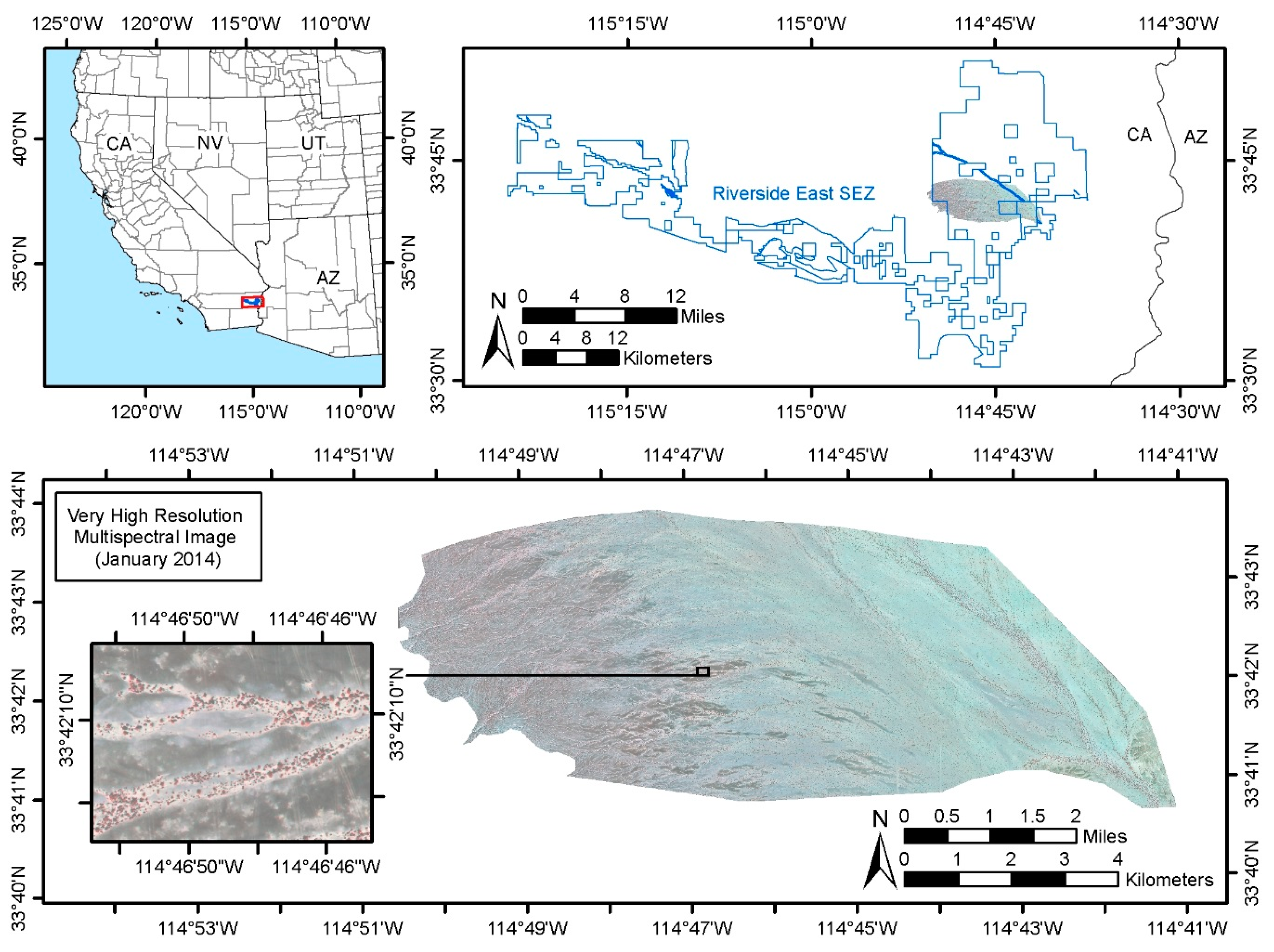
The study area is located in Palo Verde Mesa in eastern Riverside County, California (Figure 1). It covers approximately 60 km2 within the Riverside East solar energy zone [32]. Riverside East solar energy zone was identified in 2012 and includes a total area of approximately 600 km2 [9]. As of November 2018, the Riverside East solar energy zone included areas of four operational solar energy facilities (totaling 1285 MW operating capacity), as well as four projects with projected capacity of up to 1400 MW that are in the pre-construction stages (i.e., pending or approved) [33].
The ground surface of the study area consists mainly of erodible soils mixed with desert pavement and sparsely distributed vegetation. Approximately 25% of the area to the west shows rugged terrain having the highest elevation of 315 m. The rest of study area has a gentle slope toward dry wash (the McCoy Wash) at the foothills to the east with the lowest elevation of 185 m [32,34]. The study area falls within the Sonoran Desert, which exhibits two distinct wet seasons, a summer monsoon season having intense storms and a winter rainy season having scattered low-intensity precipitation [35]. The average annual precipitation of the area is 9.7 cm. The average maximum temperature in the warmest month and the average minimum temperature in the coldest month are 42.5 °C in July and 3.5 °C in January, respectively [36].
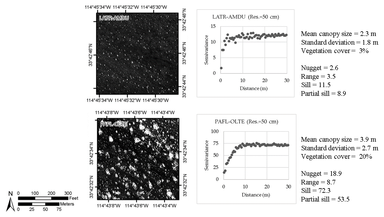
The area is primarily covered by bare ground with sparsely distributed vegetation that consists of desert scrub species (e.g., creosote bush (Larrea tridentata) and white bursage (Ambrosia dumosa)), microphyll trees (e.g., blue palo verde (Parkinsonia florida) and ironwood (Olneya tesota)), perennial grass, such as galleta grass (Pleuraphis rigida or Hilaria rigida), and annual forbs, such as desert sunflower (Geraea canescens). Four vegetation alliances (Chorizanthe rigida–Geraea canescens (CHRI–GECA), Larrea tridentata–Ambrosia dumosa (LATR–AMDU), Larrea tridentate–Encelia farinosa (LATR–ENFA), and Parkinsonia florida–Olneya tesota (PAFL–OLTE)) represent dominant habitat types in the study area (Table 1). LATR–ENFA is a shrub-dominant habitat that exhibits small yet moderate cover of vegetation having directional patterns associated with slope. The habitat occurs in mountain-front areas located in the western portion of the study area. PAFL–OLTE is a major riparian habitat within dry wash in the eastern portion of the study area. The habitat exhibits larger canopy sizes characterized by microphyll trees mixed with varying-size shrubs and herbaceous plants. CHRI–GECA and LATR–AMDU cover areas between LATF–ENFA at the highest elevation and PAFL–OLTE at the lowest elevation in the study area. CHRI–GECA is a herb-dominant habitat occurring east of LATE–ENFA. The habitat contains linear distributions of plants concentrated along ephemeral streams. LATR–AMDU is the most abundant shrub-dominant habitat occuring just west of PAFL–OLTE. The habitat exhibits repetitive patterns of shrubs with constant spacing across the landscape.
2.2. Data
For our previous study [32], VHSR multispectral images of the study area were collected on January 15 and 16, 2014, from a lightweight, fixed-wing sport aircraft approximately 1350 m above the ground. The 15 cm resolution images consisted of four spectral bands within the visible and near-infrared (NIR) spectral regions. A total of 1572 image frames were radiometrically corrected, mosaicked, orthorectified, and clipped to the study extent. The time of image collection, while unconventional for a vegetation study, is consistent with the recommendations of a recent report published by a land management agency summarizing a long-term environmental monitoring strategy for the study area [12].
To select and sample vegetation alliances, we used the vegetation alliance map available from the California Department of Fish and Wildlife, Vegetation Classification and Mapping Program, which was generated by digitizing vegetation alliances found on 2010 National Agricultural Imagery Program (NAIP) imagery [37]. We used the land cover classification map generated in our previous study [32] to obtain contextual information about the vegetation alliances. The land cover classes represented in the map include tree, shrub, desert varnish, pebble, and bare soil.
Plant canopy diameter was recorded in the field from a total of 37 plots in March 2015 using the three-transect method [38,39] and a 30 m transect. For areas with no clear physical transition in landscape, we used a plot with a spoke design containing three transects (circular plot); for areas containing ephemeral channels or riparian corridors, we adopted a design consisting of three transects perpendicular to the channel or corridor (riparian plot) [32]. Despite the 13-month time lag between image collection and field survey, the field data could serve as a reference dataset for this study because arid vegetation, particularly woody plants, grows very slowly, and its properties, such as average canopy size and spatial distribution, are relatively stable over time without catastrophic events (e.g., historical drought, flood, and land clearing) [40,41].
2.3. Image Preparation
In the previous study [32], the 8-bit VHSR imagery having pixel values ranging from 0 to 255 was transformed to represent surface reflectance ranging from 0 to 100 using surface reflectance values collected during the field work from clearly identifiable pseudo-invariant features in the image. In the same study, the Visible Atmospherically Resistant Index (VARI) was computed using the reflectance image based on Equation (1) [42]:
where Rgreen, Rred, and Rblue are reflectance or pixel values of the green, red, and blue spectral band of the image, respectively. In the previous study [32], we examined ten widely utilized spectral vegetation indices for their ability to identify vegetation in arid environments in order to map vegetation cover in the study area. The results from two independent years indicated that the VARI had higher accuracy in detecting vegetation features in the desert landscape, and its detection accuracy was most consistent across the two years of the ten indices tested. Thus, the VARI was selected for this study instead of other vegetation indices. To create study plots, we overlaid a 150 m × 150 m grid on the VARI image to partition the landscape into 22,500 m2 plots. This plot size provided sufficient areal extent to capture spatial patterns in each alliance.
2.4. Analyses
The spatial structure of the four vegetation alliances—LATR–ENFA, CHRI–GECA, LATR–AMUD, and PAFL–OLTE—was analyzed using variograms. The variogram is a geostatistical tool that measures spatial continuity and quantitatively describes spatial autocorrelation in the data [28,43]. The measured spatial pattern is often expressed as semivariance (γ). Semivariance is one half the average squared difference of data values for every pair of locations, and it is calculated using Equation (2):
where xi is a location of a data point, Z(x) is the data value at location x, h is a unit distance between a set of points that defines the lag h, and N is the number of data pairs that are h distance apart (Table 2). The lag or lag increment defines the distance at which a variogram is computed. Because the distance between two points may not exactly match the lag, bins (which are defined by the lag and a lag tolerance) are used instead of exact distances when constructing the variogram [44]. The lag tolerance is typically isotropic and often is half the distance between lags so that all possible pairs are included. The semivariances are plotted against the distance between locations to construct a variogram. Using the variogram generated from actual data (experimental variogram), a modeled variogram was formulated by fitting an appropriate theoretical variogram model that is associated with known mathematical properties. Increasing the lag tends to smooth the variogram because the bin width, which defines the distance for averaging semivariances, linearly correlates to the lag. We examined the sensitivity of the variogram parameters to increased lag sizes and investigated how those sensitivities of the variogram parameters would affect its indicative power of intrinsic spatial structure of desert vegetation communities.
The variogram that is derived from remotely sensed imagery provides graphical representation of overall variability in the image as a function of the distance between pixels [23,45]. When a variogram is generated using a spectral vegetation index, its parameters are indicative of the spatial structure of vegetated landscape [23,45]. When internal structures of vegetation communities change, the variogram properties—such as range, sill, and form—change accordingly; thus, they would be useful indicators for monitoring the internal conditions of vegetation alliances.
Three VARI image plots were selected within each of the four vegetation alliances [46]. To analyze the spatial patterns of vegetation, the VARI values in the plots were extracted, and the data that shared a common vegetation alliance were pooled to create a single dataset for each alliance. Experimental variograms were calculated for each alliance using the pooled data by applying nine lags—15 cm, 30 cm, 50 cm, 1 m, 1.5 m, 2.5 m, 5 m, 10 m, and 15 m. For each alliance, an appropriate model variogram was selected interactively by fitting the experimental variogram. Variogram parameters, such as form, nugget, range, sill, and partial sill, were identified and related to the landscape properties associated with each alliance.
To examine the effects of image resolution on interpretability of intrinsic spatial structure of the vegetation alliances, we generated VARI images having four spatial scales—30 cm, 50 cm, 1 m, and 1.5 m—by spatially aggregating the original 15-cm resolution image into the target resolutions. All pixel values within each target spatial scale were averaged first, and then the index was computed. For each spatial scale, VARI values in the plots were extracted, and the data that shared a common vegetation alliance were pooled to create a single dataset for each alliance. Using the datasets, we calculated an experimental variogram, selected the best fit variogram model, and extracted variogram parameters (i.e., form, range, nugget, sill, and partial sill) for each vegetation alliance. We examined how well the landscape structures that were observed at the original image resolution were preserved to determine appropriate spatial resolutions for monitoring changes in the vegetation alliances. All variograms were computed using the ESRI ArcMap 10.7 semivariogram tool (http://desktop.arcgis.com/en/arcmap/latest/extensions/geostatistical-analyst/modeling-a-semivariogram.htm).
3. Results and Discussion
3.1. Variogram Parameters for Vegetation Alliances Across Lags
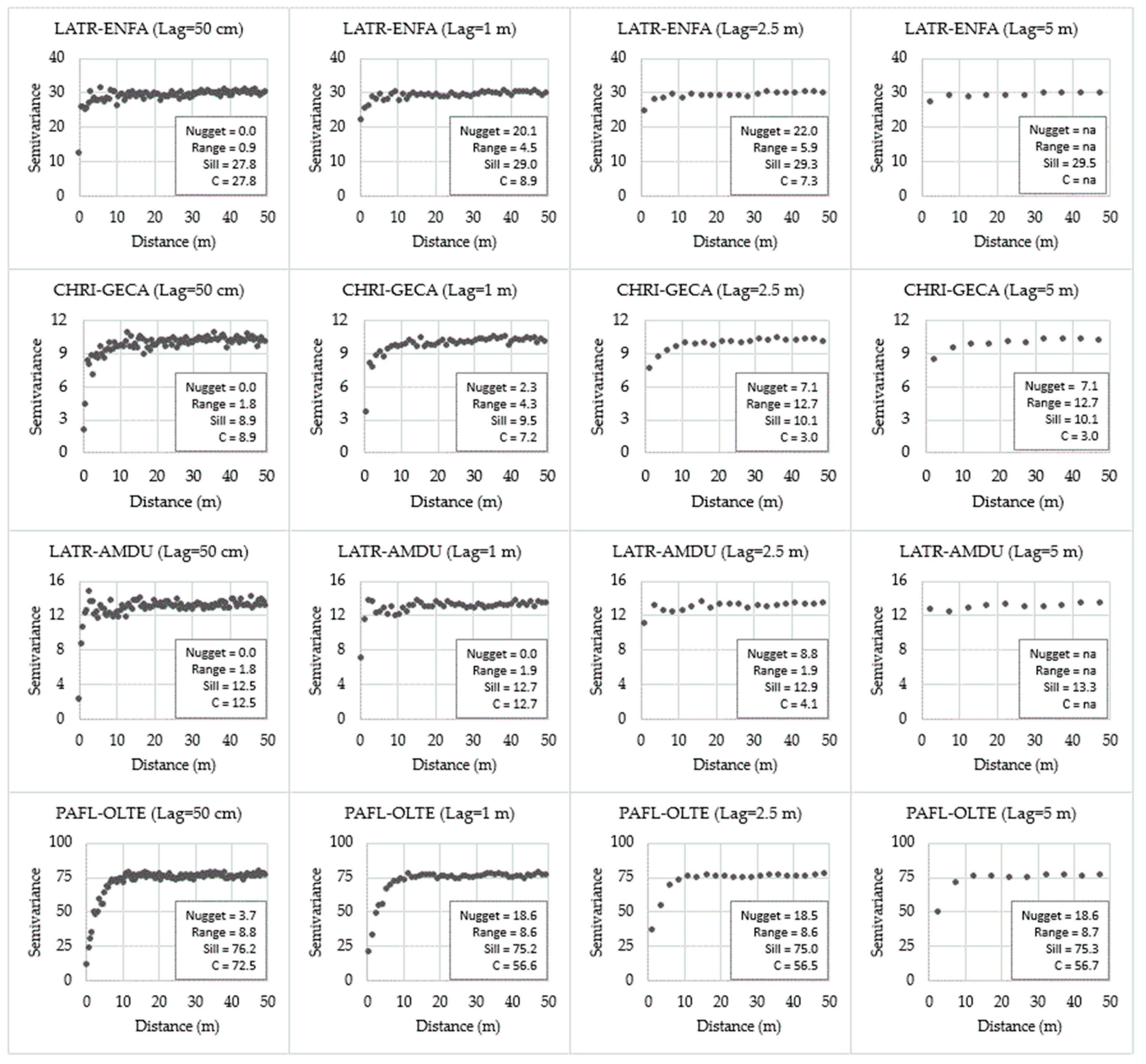
Experimental variograms for the four vegetation alliances—LATR–ENFA, CHRI–GECA, LATR–AMUD, and PAFL–OLTE—with selected lags—50 cm, 1 m, 2.5 m and 5 m—are shown in Figure 2. Experimental variograms for all lags examined are presented in Supplemental Material (Figure S1). All variograms for the four alliances show either spherical or exponential form across most of the lags. The spherical form is characterized by the semivariance increasing at a relatively constant rate and plateauing when reaching the sill. The exponential form is characterized by the semivariance gradually increasing and forming a smooth curve when reaching the sill. Alliances dominated by shrubs and forbs, such as LATR–ENFA, CHRI–GECA, and LATR–AMDU, share a spherical form, while PAFL–OLTE has an exponential form, which likely reflects varying canopy size within the habitat (Figure S1). In fact, the standard deviation of canopy size for PAFL–OLTE is the greatest of all alliances (2.7 m, Table 1). The shape and characteristics of variograms become obscure as the lag increases.
The sill remains nearly constant across the lags for all alliances, which indicates that the sill is relatively insensitive to averaging of semivariances through increasing the bin widths or lag sizes. Thus, intrinsic vegetation density or cover of each alliance can be captured with any lag sizes within the lags examined (Figure 2). The partial sill becomes increasingly smaller as the lag size increases, which suggests that variation within the landscape associated with spatial structure becomes difficult to observe when a large lag size is applied. Spatial structure becomes indistinguishable across the shrub- or forb-dominant habitats (i.e., LATR–ENFA, CHRI–GECA, and LATR–AMUD) when a lag of 1 m or greater is used. Very sparsely vegetated alliances, such as CHRI–GECA (7%) and LATR–AMDU (3%), tend to have sills lower than 13 (Table 1 and Figure 2), which is considerably low compared with LATR–ENFA (18%) and PAFL-OLTE (20%), where sills are higher than 27 (Table 1 and Figure 2).
At the 50 cm lag, the range relates to the average canopy size across the alliances. LATR–ENFA, which is characterized by small shrubs (average canopy diameter = 1.5 m) has the smallest range (0.9 m), and PAFL–OLTE that consists of trees and large shrubs (average canopy diameter = 3.9 m) has the largest range (8.8 m) (Table 1 and Figure 2). However, the relationship begins to dissipate at the 1 m lag; thus, the range calculated with a lag of 1 m or greater would not be indicative of the average canopy size within the alliance.
LATR–ENFA, which is characterized by moderate cover of small shrubs (Table 1), appears to lose its characteristic variogram parameters beyond the 50 cm lag, such as the range indicative of canopy size and the partial sill indicative of spatial structure (Figure 2). This suggests that the range and partial sill of this alliance are sensitive to smoothing, and a lag of 50 cm or smaller would be needed in order to observe spatial structure of the alliance. However, the sill indicative of vegetation cover remains constant around 20, regardless of the lag.
PAFL–OLTE containing trees and large shrubs (Table 1) maintains its distinct variogram parameters even at the 5 m lag, including range, sill, and partial sill, despite the noticeable changes in nugget and partial sill when transposing the lag from 50 cm to 1 m (Figure 2). This means that those variogram parameters are relatively robust to smoothing, and the habitat characteristics, such as canopy size, vegetation cover, and spatial structure, can be examined using a relatively large lag compared to other alliances.
CHRI–GECA, characterized by very sparse herbaceous cover, and LATR–AMDU, characterized by very sparse shrub cover (Table 1), appear to mostly maintain their characteristic variogram parameters with lags up to 1 m (Figure 2). Thus, the habitat characteristics, such as canopy size, vegetation cover, and spatial structure, could be characterized using a lag up to 1 m for these two sparsely vegetated alliances.
Based on the observations above, the lag analysis confirmed that the published relationships between variogram parameters and landscape properties [23,45] hold true for the desert landscape examined in this study. When using a remotely-sensed vegetation index, variogram parameters are indicative of the spatial structure of vegetation in the landscape. The variogram form indicates variability of plant canopy sizes, the sill corresponds to overall vegetation cover or density within each alliance, and the range relates to the average canopy size in a relative sense.
Averaging effects or smoothing of semivariances associated with bin widths or lag sizes has varying impacts on the variogram parameters and on alliance types. While the sill appears relatively insensitive, the partial sill is sensitive to increased bin widths because the nugget (indicating random variation in the data) becomes increasingly high when averaging over a larger bin width. These observations suggest that overall vegetation cover would be characterized relatively well, regardless of the lag across the community types, but characterizing spatial structure of the communities would require a small lag. The range appears sensitive to smoothing, and the intrinsic range quickly dissipates when a larger bin width is applied. This suggests that the average canopy size within the communities needs to be considered when selecting an appropriate lag. When considering the average canopy size, the variogram parameters of the alliance having the largest average canopy size (PAFL–OLTE) appear insensitive, while those of the alliance having the smallest average canopy size (LATR–ENFA) exhibit extreme sensitivity to smoothing. This observation clearly suggests that a small lag (~50 cm) would be required to effectively characterize intrinsic landscape structure of habitats dominated by small plants. Overall, quantifying characteristic spatial structure for each of the four alliances in a single image would require a 50 cm or smaller lag.
3.2. Variogram Parameters for Vegetation Alliances Across Image Resolutions
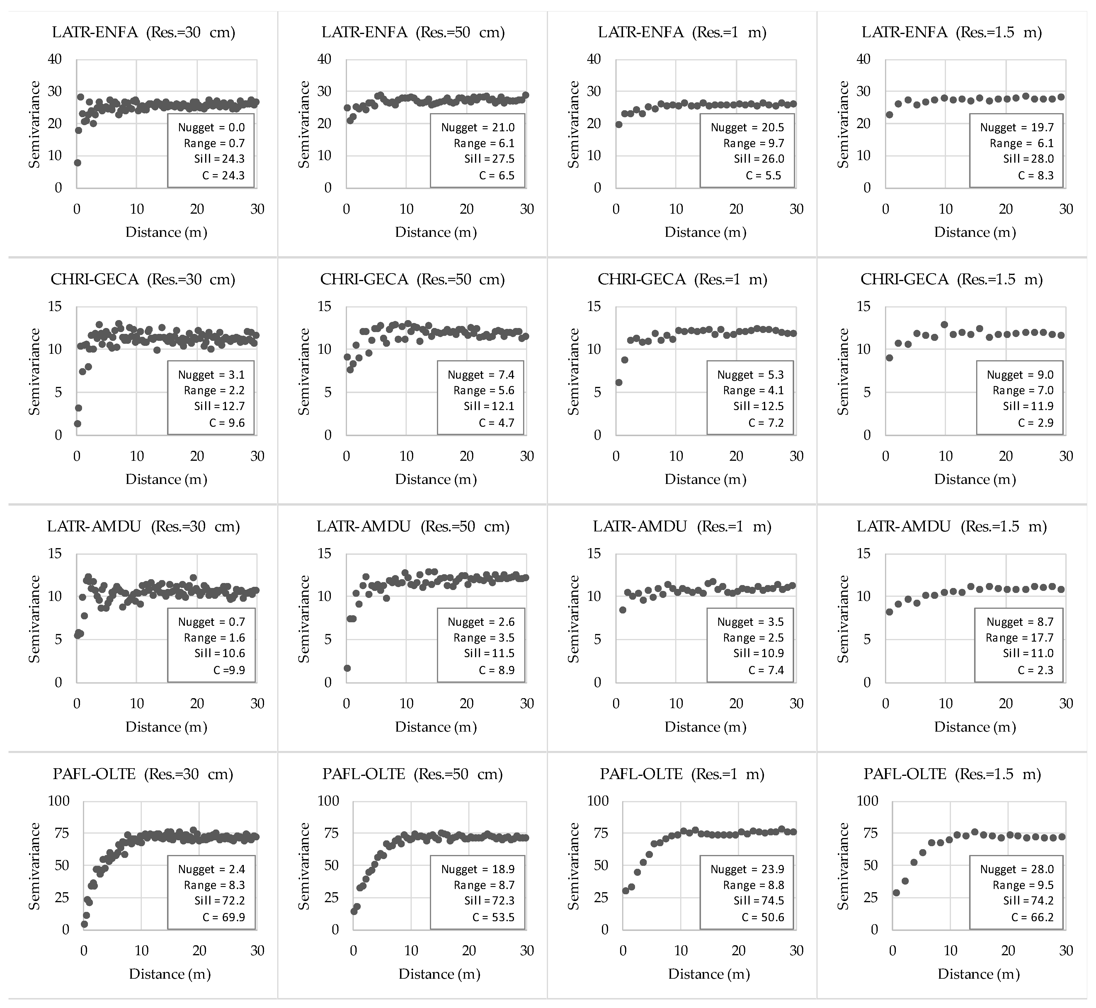
Experimental variograms for the four vegetation alliances—LATR–ENFA, CHRI–GECA, LATR–AMUD, and PAFL–OLTE—examined at four spatial resolutions—30 cm, 50 cm, 1 m, and 1.5 m—are shown in Figure 3. Characteristic variogram parameters of each alliance, such as the range indicative of average canopy size and the partial sill indicative of spatial structure, become increasingly obscure as spatial resolution coarsens. This suggests that characteristic landscape properties and structure are not observable when using images having coarse spatial resolution. The sill remains constant across the spatial resolutions examined, which indicates that the vegetation cover or density can be characterized even at 1.5 m resolution.
When comparing the spatial-resolution analysis (Figure 3) and the lag analysis (Figure 2 and Figure S1), the variogram parameters at a comparable unit distance (e.g., 1 m spatial resolution and 1 m lag) are not comparable. For example, the partial sill is consistently higher with the 50 cm lag than that with 50 cm resolution. The range is smaller with 50 cm lag than with 50 cm resolution, except for PAFL–OLTE. These patterns indicate that landscape characteristics, such as the average canopy size and spatial structure, which are observed in a fine resolution image with 50 cm lag would not be observable in a 50-cm resolution image. The sill, on the other hand, is comparable when comparing the variogram parameters at a comparable unit distance. The partial sill generally decreases as the resolution becomes coarser across the alliances. This indicates that detection of landscape variation associated with spatial structure decreases as spatial resolution coarsening. Particularly, at spatial resolution of 1 m or coarser, variation within the landscape becomes indistinguishable among the shrub- or forb-dominant alliances (i.e., LATR–ENFA, CHRI–GECA, and LATR–AMDU). The same pattern is observed in the lag analysis (Figure 2).
For LATR–ENFA characterized by moderate cover (18%, Table 1) of small shrubs and forbs, the partial sill decreases from 24.3 to 6.5 when coarsening the spatial resolution from 30 cm to 50 cm (Figure 3). This indicates that the habitat’s intrinsic variation associated with spatial structure is no longer captured at the spatial resolution beyond 30 cm, although its overall vegetation cover is characterized by the sill, regardless of the spatial resolution. For PAFL–OLTE consisting of trees and large shrubs, the partial sill remains between 50.6 and 69.9 across the spatial resolutions, which is noticeably greater than that of other alliances (Figure 3). This suggests that for this vegetation alliance, landscape variation associated with spatial structure can be detected with 1.5 m or finer spatial resolution. The shape of the variogram appears exponential compared to that of other alliances, indicating greater canopy size variation (standard deviation = 2.7, Table 1).
3.3. Synthesis
It is clear that the LATR–ENFA alliance characterized by a small canopy size would require 50 cm or finer resolution to capture most of its inherent landscape characteristics. The CHRI–GECA and LATR–AMDU alliances that share similarities in landscape properties produced very similar variogram parameters. Although this could present a limitation when classifying habitat types, this result would be an indication of robust relationships between variogram parameters and landscape properties, regardless of habitat types.
The PAFL–OLTE alliance has consistent variogram parameters across a range of image resolutions. Thus, a variogram technique applied using publicly available imagery, such as NAIP imagery (60 cm~1 m), could provide useful information for detecting and monitoring internal changes in the alliance, such as changes in overall vegetation cover and canopy (e.g., degradation of shrubs, reduction of tree canopy size). Contrasting variogram forms between the tree-dominant PAFL–OLTE alliance and other shrub- and herb-dominant alliances suggests that the variogram form of PAFL–OLTE is expected to shift from an exponential form to a spherical form when canopy size diversity declines. In the context of monitoring of the Riverside East solar energy zone, a possible scenario that could be detected would be a reduction in tree abundance and size and an increase in shrub dominance in a part of the major ephemeral stream due to a change in surface water flow.
One of the most promising landscape properties that can be monitored using a variogram technique is vegetation cover within an alliance. Despite smoothing effects induced by large lags and coarse spatial resolutions, the sill appears to maintain its intrinsic height across the vegetation alliances. Thus, changes in vegetation cover can likely be detected using a range of lags and spatial resolutions. However, it should be noted that the sill cannot be directly interpreted as absolute fractional vegetation cover. In this study, the LATR–ENFA and PAFL–OLTE alliances that have similar vegetation cover (18% and 20%, respectively, Table 1) had very different sills (Figure 2 and Figure 3). Therefore, it is essential to establish a baseline sill for each alliance as an indicator of fractional vegetation cover at the initiation of monitoring. Very different sills for comparable vegetation cover may be partly attributed to differences in vegetation greenness since variograms were generated from a spectral vegetation index. If this is true, the sill could indicate habitat health, as well as vegetation cover within the habitat. This hypothesis warrants further study.
When monitoring the four alliances using a single image, LATR–ENFA—having the smallest average canopy size—would determine an appropriate image resolution, which is likely the least cost-effective image type due to its fine image resolution. For sustainable long-term monitoring, this consideration is important for prioritizing monitoring efforts, such as what or how many habitats, how often, and how extensively to monitor using a variogram technique.
The comparison of variogram parameters between the lag analysis and the image-resolution analysis revealed a potential problem with determining an appropriate image resolution for applying a variogram technique to monitoring landscape structure changes. A lag up to 50 cm with a 15 cm resolution image appeared to have good potential for detecting changes in characteristic spatial structure for each of the four alliances in a single image. However, it is unlikely that a 50 cm resolution image indicates the same landscape properties for the alliances, and thus an image having a finer spatial resolution would be required, particularly for habitats characterized by small canopy sizes and sparse vegetation. This discrepancy suggests that the smoothing effect induced by increased lag sizes and that induced by degraded image resolutions do not have equal impacts on the variogram. Images having 30 cm spatial resolution or finer may be useful for monitoring internal landscape changes for dryland habitats because at this resolution, variogram parameters were relatively stable across the vegetation alliances examined (Figure 3).
It should be noted that the results in this study may have been affected by the 13-month time span between image collection and field survey. However, because of desert vegetation characterized by slow-growth and drought-tolerant nature, the impact of the time lag is considered minimal.
4. Conclusions
By utilizing a fine-resolution spectral vegetation index, we examined the variogram technique for quantifying spatial structure of dryland environments using the four most abundant vegetation alliances in the Riverside East solar energy zone—one habitat characterized by moderate cover of small plants (LATR–ENFA), two habitats with very sparse vegetation cover of small or small to medium size canopies (LATR–AMDU and CHRI–GECA), and one habitat with moderate vegetation cover consisting of a range of plant sizes (PAFL–OLTE). Our aims were to (1) gain insights into whether or not a variogram technique has the potential to detect subtle changes in properties of desert vegetation habitats; (2) understand trade-offs between image resolution and detectable changes within each desert habitat type; and (3) determine considerations for the application of a variogram method for dryland monitoring. The findings from this study conducted in the desert region of the southwestern United States could apply to other desert environments. Key findings likely applicable for many desert regions are summarized as follows:
- Variogram parameters that are generated from a spectral vegetation index using fine resolution imagery can provide information about unique, intrinsic characteristics of dryland habitats. The sill, range, form, and partial sill of the variogram relate to overall vegetation cover or density, average canopy size, canopy size variation, and spatial structure of plants within a habitat, respectively, which are consistent with published studies [23,27,45].
- Establishing a baseline of variogram parameters for each habitat is an important first step of monitoring because variogram parameters do not indicate absolute values of landscape properties, and they may be similar or indistinguishable between habitat types that have a similar canopy size. Comparing variogram parameters of each habitat against their baselines could indicate internal change within the habitat (e.g., vegetation cover, average canopy size, and canopy size variation). However, understanding the magnitude of changes detectable using variogram parameters requires additional studies.
- For the variogram generated from a spectral vegetation index, the sill may be influenced by vegetation greenness, which could indicate the health of vegetation communities. If we can successfully detect changes in habitat conditions using remote sensing, it could greatly contribute to monitoring of extensive desert lands over time in a financially sustainable manner by substantially reducing field-based monitoring costs. To determine the effectiveness of variograms for monitoring vegetation community health, further studies are warranted.
For monitoring landscape changes, field survey and traditional image processing methods would continue to play an important role in monitoring landscape changes. The variogram technique demonstrated in this study could provide complementary knowledge on the spatial structure of the vegetated landscape, which is difficult to obtain from traditional monitoring methods.
Once the baseline variogram is established, periodic variogram analysis using publicly available imagery (e.g., 60 cm resolution NAIP imagery), commercially available fine spatial resolution imagery (e.g., 30~50 cm resolution WorldView-3 imagery), or custom very fine resolution imagery using unmanned aerial systems, or UASs, could reduce the required frequency of field data collection. Because of the accessibility of these fine resolution image options, a variogram technique is now considered a viable option for cost-effective long-term environmental monitoring. A combination of land cover information obtained from existing monitoring methods and spatial structure information extracted from the variogram analysis could improve effectiveness and timeliness of detection and monitoring of desert land landscape changes.
Supplementary Materials
The following are available online at https://www.mdpi.com/2072-4292/11/12/1495/s1, Figure S1. Semivariograms of the LATR ENFA, CHRI–GECA, LATR–AMDU, and PAFL–OLTE alliances with all lags tested—15 cm, 30 cm, 50 cm, 1 m, 1.5 m, 2.5 m, 5 m, 10 m and 15 m.
Author Contributions
Conceptualization, Y.H.; Data curation, K.S.; Formal analysis, Y.H.; Funding acquisition, H.M.H.; Investigation, Y.H.; Methodology, Y.H.; Project administration, M.G. and H.M.H.; Supervision, M.G.; Validation, Y.H.; Visualization, K.S.; Writing—original draft, Y.H.; Writing—review & editing, K.S., M.G. and H.M.H.
Funding
This research was funded by the U.S. Department of Interior, Bureau of Land Management, agreement number L17PG00209.
Acknowledgments
The authors thank all anonymous reviewers who provided valuable feedback and constructive criticism to improve the quality of the article.
Conflicts of Interest
The authors declare no conflict of interest.
References
- Le Houerou, H.N. Climate change, drought and desertification. J. Arid Environ. 1996, 24, 133–185. [Google Scholar] [CrossRef]
- Oerter, E.; Mills, J.V.; Maurer, G.E.; Lammers, L.N.; Amundson, R. Greenhouse Gas Production and Transport in Desert Soils of the Southwestern United States. Glob. Biogeochem. Cycles 2018, 32, 1703–1717. [Google Scholar] [CrossRef]
- Intergovernmental Panel on Climate Change (IPCC). Climate Change 2013: The Physical Science Basis; Contribution of Working Group I to the Fifth Assessment Report of the IPCC; Stocker, T.F., Qin, D., Plattner, G.-K., Tignor, M., Allen, S.K., Boshung, J., Nauels, A., Xia, Y., Bex, V., Midgley, P.M., Eds.; Cambridge University Press: Cambridge, UK, 2013; 1533p. [Google Scholar] [CrossRef]
- Intergovernmental Panel on Climate Change (IPCC). Summary for policymakers. In Climate Change 2014: Impacts, Adaptation, and Vulnerability. Part A: Global and Sectoral Aspects; Contribution of Working Group II to the Fifth Assessment Report of the IPCC; Field, C.B., Barros, V.R., Dokken, D.J., Mach, K.J., Mastrandrea, M.D., Bilir, T.E., Chatterjee, M., Ebi, K.L., Estrada, Y.O., Genova, R.C., et al., Eds.; Cambridge University Press: Cambridge, UK, 2014; 151p. [Google Scholar] [CrossRef]
- Thomas, J.; El-Sheikh, M.A.; Alfarhan, A.H.; Alatar, A.A.; Sivadasan, M.; Basahi, M.; Al-Obaidm, S.; Rajakrishnan, R. Impact of alien invasive species on habitats and species richness in Saudi Arabia. J. Arid Environ. 2016, 127, 53–65. [Google Scholar] [CrossRef]
- Zhang, R.; Wang, Z.; Han, G.; Schellenberg, M.P.; Wu, Q.; Gu, C. Grazing induced changes in plant diversity is a critical factor controlling grassland productivity in the Desert Steppe, Northern China. Agric. Ecosyst. Environ. 2018, 265, 73–83. [Google Scholar] [CrossRef]
- Rowe, H.I.; Tluczek, M.; Broatch, J.; Gruber, D.; Jones, S.; Langenfeld, D.; McNamara, P.; Weinstein, L. Comparison of trailside degradation across a gradient of trail use in the Sonoran Desert. J. Environ. Manag. 2018, 207, 292–302. [Google Scholar] [CrossRef]
- Amponsah, N.Y.; Troldborg, M.; Kington, B.; Aalders, I.; Hough, R.L. Greenhouse gas emissions from renewable energy sources: A review of lifecycle considerations. Renew. Sustain. Energy Rev. 2014, 39, 461–475. [Google Scholar] [CrossRef]
- Bureau of Land Management (BLM). Approved Resource Management Plan Amendments/Record of Decision (ROD) for Solar Energy Development in Six Southwestern States; U.S. Department of the Interior, BLM: Washington, DC, USA, 2012.
- Barron-Gafford, G.A.; Minor, R.L.; Allen, N.A.; Cronin, A.D.; Borrks, A.E.; Pavao-Zuckerman, M.A. The Photovoltaic Heat Island Effect: Larger solar power plants increase local temperatures. Sci. Rep. 2016, 6, 35070. [Google Scholar] [CrossRef] [Green Version]
- Hernandez, R.R.; Hoffacker, M.K.; Murphy-Mariscal, M.L.; Wu, G.C.; Allen, M.F. Solar energy development impacts on land cover change and protected areas. Proc. Natl. Acad. Sci. USA 2015, 112, 13579–13584. [Google Scholar] [CrossRef] [Green Version]
- BLM. Riverside East Solar Energy Zone Long Term Monitoring Strategy: Final Report; U.S. Department of Interior, BLM: Washington, DC, USA, March 2016.
- Taylor, J.J.; Kachergis, E.J.; Toves, G.R.; Karl, J.W.; Bobo, M.R.; Karl, M.; Millar, S.; Spurrier, C.S. AIM-Monitoring: A Component of the BLM Assessment, Inventory, and Monitoring Strategy; Technical Note 445; U.S. Department of the Interior, Bureau of Land Management, National Operations Center: Denver, CO, USA, 2014.
- Bunce, R.G.H.; Metzger, M.J.; Jongman, R.H.G.; Brandt, J.; De Blust, G.; Elena-Rossello, R.; Groom, G.B.; Halada, L.; Hofer, G.; Howard, D.C.; et al. A standardized procedure for surveillance and monitoring European habitats and provision of spatial data. Landsc. Ecol. 2008, 23, 11–25. [Google Scholar] [CrossRef]
- McCord, S.E.; Buenemann, M.; Karl, J.W.; Browning, D.M.; Hadley, B.C. Integrating remotely sensed imagery and existing multiscale field data to derive rangeland indicators: Application of Bayesian additive regression trees. Rangel. Ecol. Manag. 2017, 70, 644–655. [Google Scholar] [CrossRef]
- Ksiksi, T.S.; El-Keblawy, A.A. Floral diversity in desert ecosystems: Comparing field sampling to image analyses in assessing species cover. BMC Ecol. 2013, 13. [Google Scholar] [CrossRef]
- Duniway, M.C.; Karl, J.W.; Schrader, S.; Baquera, N.; Herrick, J.E. Rangeland and Pasture Monitoring: An Approach to Interpretation of High-Resolution Imagery Focused on Observer Calibration for Repeatability. Environ. Monit. Assess. 2012, 184, 3789–3804. [Google Scholar] [CrossRef]
- Kilpatrick, A.D.; Lewis, M.M.; Ostendorf, B. Rangeland condition monitoring: A new approach using cross-fence comparisons of remotely sensed vegetation. PLoS ONE 2015, 10, e0142742. [Google Scholar] [CrossRef]
- Godinez-Alvarez, H.; Herrick, J.E.; Mattocks, M.; Toledo, D.; Van Zee, J. Comparison of three vegetation monitoring methods; their relative utility for ecological assessment and monitoring. Ecol. Indic. 2009, 9, 1001–1008. [Google Scholar] [CrossRef]
- Ustin, S.L.; Jacquemond, S.; Palacios-Orueta, A.; Li, L.; Whiting, M.L. Remote sensing based assessment of biophysical indicators for land degradation and desertification. In Recent Advances in Remote Sensing and Geoinfomration Processing for Land Degradation Assessment; Roeder, A., Hill, J., Eds.; ISPRS Series: London, UK, 2009; pp. 15–44. [Google Scholar] [Green Version]
- Hamada, Y.; Stow, D.A.; Robert, D.A.; Franklin, J.; Kyriakidis, P.S. Assessing and monitoring semi-arid shrublands using object-based image analysis and multiple endmember spectral mixture analysis. Environ. Monit. Assess. 2013, 185, 3173–3190. [Google Scholar] [CrossRef] [PubMed]
- Frieswyk, C.B.; Johnston, C.A.; Zedler, J.B. Identifying and characterizing dominant plans as an indicator of community condition. J. Great Lakes Res. 2007, 33 (Suppl. 3), 125–135. [Google Scholar] [CrossRef]
- Phinn, S.; Franklin, J.; Hope, A.; Stow, D.; Huenneke, L. Biomass distribution mapping using airborne digital video imagery and spatial statistics in a semi-arid environment. J. Environ. Manag. 1996, 47, 139–164. [Google Scholar] [CrossRef]
- Schlesinger, W.H.; Reynolds, J.F.; Cunningham, G.L.; Huenneke, L.F.; Jarrell, W.J.; Virginia, R.A.; Whitford, W.G. Biological feedbacks in global desertification. Science 1990, 247, 1043–1048. [Google Scholar] [CrossRef]
- Roughgarden, J.; Running, S.W.; Matson, P.A. What does remote sensing do for ecology? Ecology 1991, 72, 1918–1922. [Google Scholar] [CrossRef]
- Ustin, S.L.; Smith, M.O.; Adams, J.B. Remote sensing of ecological processes: A strategy for developing and testing ecological models using spectral mixture analysis. In Scaling Physiological Processes: Leaf to Globe; Ehleringer, J.R., Field, C.B., Eds.; Academic Press: San Diego, CA, USA, 1993; pp. 339–357. [Google Scholar]
- Wallace, C.S.; Watts, J.J.; Yool, S.R. Characterizing the spatial structure of vegetation communities in the Mojave Desert using geostatistical techniques. Comput. Geosci. 2000, 26, 397–410. [Google Scholar] [CrossRef]
- Cressie, N. Statistics of Spatial Data; Wiley: New York, NY, USA, 1993; 900p. [Google Scholar]
- Garrigues, S.; Allard, D.; Baret, F.; Morisette, J. Multivariate quantification of landscape spatial heterogeneity using variogram models. Remote Sens. Environ. 2008, 112, 216–230. [Google Scholar] [CrossRef]
- Guo, H.; Jiapaera, G.; Baoa, A.; Li, X.; Huanga, Y.; Ndayisaba, F.; Menga, F. Effects of the Tarim River’s middle stream water transport dike on the fractional cover of desert riparian vegetation. Ecol. Eng. 2017, 99, 333–342. [Google Scholar] [CrossRef]
- Raynor, E.J.; Griffith, C.D.; Twidwell, D.; Schacht, W.H.; Wonkka, C.L.; Roberts, C.P.; Bielski, C.L.; Debinski, D.M.; Miller, J.R. The emergence of heterogeneity in invasive-dominated grassland: A matter of the scale of detection. Landsc. Ecol. 2018, 33, 2013–2119. [Google Scholar] [CrossRef]
- Hamada, Y.; Grippo, M.A.; Smith, K.P. Long-Term Monitoring of Utility-Scale Energy Development and Application of Remote Sensing Technologies: Summary Report; ANL/EVS-14/12; Argonne National Laboratory: Lemont, IL, USA, 2014. [Google Scholar]
- BLM. Solar Energy Project Information. Available online: https://www.blm.gov/sites/blm.gov/files/energy_renewable_SolarProjectInfo_november%202018%20%282%29_0.xlsx (accessed on 22 June 2019).
- Hamada, Y.; O’Connor, B.L.; Orr, A.B.; Wuthrich, K.K. Mapping ephemeral stream networks in desert environments using very-high-spatial-resolution multispectral remote sensing. J. Arid Environ. 2016, 130, 40–48. [Google Scholar] [CrossRef] [Green Version]
- Reynolds, J.F.; Kemp, P.R.; Ogle, K.; Fernández, R.J. Modifying the Pulse-Reserve’ Paradigm for Deserts of North America: Precipitation Pulses, Soil Water, and Plant Responses. Oecologia 2004, 141, 194–210. [Google Scholar] [CrossRef]
- Western Regional Climate Center. Available online: https://wrcc.dri.edu/cgi-bin/cliMAIN.pl?cablyt+sca (accessed on 31 May 2016).
- California Department of Fish and Wildlife (CDFW). California Desert Vegetation Map and Accuracy Assessment in Support of the Desert Renewable Energy Conservation Plan; CDFW: Sacramento, CA, USA, 2013. [Google Scholar]
- Herrick, J.E.; Van Zee, J.W.; Havstad, K.M.; Burkett, L.M.; Whitford, W.G. Monitoring Manual for Grassland, Shrubland and Savanna Ecosystems, Vol. I: Quick Start; USDA-ARS Jornada Experimental Range: Las Cruces, NM, USA, 2005. [Google Scholar]
- Herrick, J.E.; Van Zee, J.W.; Havstad, K.M.; Burkett, L.M.; Whitford, W.G. Monitoring Manual for Grassland, Shrubland and Savanna Ecosystems, Vol. II: Design, Supplementary Methods for Interpretation; USDA-ARS Jornada Experimental Range: Las Cruces, NM, USA, 2005. [Google Scholar]
- Cody, M.L. Slow-motion population dynamics in Mojave Desert perennial plants. J. Veg. Sci. 2000, 11, 351–358. [Google Scholar] [CrossRef]
- Munson, S.M.; Webb, R.H.; Housman, D.C.; Veblen, K.E.; Nussear, K.E.; Beever, E.A.; Hartney, K.B.; Miriti, M.N.; Phillips, S.L.; Fulton, R.E.; et al. Long-term plant responses to climate are moderated by biophysical attributes in a North American desert. J. Ecol. 2015, 103, 657–668. [Google Scholar] [CrossRef]
- Gitelson, A.A.; Kaufman, Y.J.; Stark, R.; Rundquist, D. Novel algorithms for remote estimation of vegetation fraction. Remote Sens. Environ. 2002, 80, 76–87. [Google Scholar] [CrossRef] [Green Version]
- Wackernagel, H. Multivariate Geostatistics: An Introduction with Applications, 3rd ed.; Springer: Berlin, Germany, 2013; pp. 45–55. [Google Scholar]
- Deutsch, C.V.; Journel, A.G. GSLIB Geostatistical Software Library and User’s Guide, 2nd ed.; Applied Geostatistics Series; Oxford University Press: New York, NY, USA, 1998. [Google Scholar]
- Woodcock, C.E.; Strahler, A.H.; Jupp, D.L. The use of variograms in remote sensing: I. Scene models and simulated images. Remote. Sens. Environ. 1988, 25, 323–348. [Google Scholar] [CrossRef]
- Hamada, Y.; Rollins, K.E. Long-Term Monitoring of Desert Land and Natural Resources and Application of Remote Sensing Technologies: Final Report; ANL/EVS-16/1; Argonne National Laboratory: Lemont, IL, USA, 2016. [Google Scholar]
Figure 1.
Study area and 15-cm resolution multispectral image.

Figure 2.
Semivariograms of the LATR–ENFA, CHRI–GECA, LATR–AMDU, and PAFL–OLTE alliances with selected lags—50 cm, 1 m, 2.5 m, and 5 m. na = not applicable.
Figure 2.
Semivariograms of the LATR–ENFA, CHRI–GECA, LATR–AMDU, and PAFL–OLTE alliances with selected lags—50 cm, 1 m, 2.5 m, and 5 m. na = not applicable.

Figure 3.
Semivariograms of the LATR–ENFA, CHRI–GECA, LATR–AMDU, and PAFL–OLTE alliances with selected spatial resolutions of imagery—30 cm, 50 cm, 1 m, and 1.5 m. na = not applicable.
Figure 3.
Semivariograms of the LATR–ENFA, CHRI–GECA, LATR–AMDU, and PAFL–OLTE alliances with selected spatial resolutions of imagery—30 cm, 50 cm, 1 m, and 1.5 m. na = not applicable.


Table 1.
Summary of four vegetation alliances examined in this study.
| Alliance (Acronym) | Visible Atmospherically Resistant Index (VARI) Image | Average Vegetation Cover | Canopy Diameter | |
|---|---|---|---|---|
| Mean | Standard Deviation | |||
| Larrea tridentata–Encelia farinosa (LATR–ENFA) |  | 18% | 1.5 m | 0.8 m |
| Chorizanthe rigida–Geraea canescens (CHRI–GECA) |  | 7% | 2.5 m | 2.2 m |
| Larrea tridentata–Ambrosia dumosa (LATR–AMDU) |  | 3% | 2.3 m | 1.8 m |
| Parkinsonia florida–Olneya tesota (PAFL–OLTE) |  | 20% | 3.9 m | 2.7 m |
Table 2.
Summary of variogram and its parameters (adapted from [28]).
Table 2.
Summary of variogram and its parameters (adapted from [28]).
| Variogram | Parameter and Definition | Indication |
|---|---|---|
 | Form: Nature of spatial variability within the data | Pattern of features in the landscape and variance distribution of landscape features |
| Range: Distance over which data are correlated | Size of dominant features in the landscape | |
| Sill: Total variation in the data | Density of features or background in the landscape | |
| Nugget: Level of random variation in the data | Variation in the landscape NOT explained by distance | |
| Partial sill: Variation associated with spatial structure defined as [Sill]–[Nugget] | Variation in the landscape explained by distance or associated with spatial autocorrelation |
© 2019 by the authors. Licensee MDPI, Basel, Switzerland. This article is an open access article distributed under the terms and conditions of the Creative Commons Attribution (CC BY) license (http://creativecommons.org/licenses/by/4.0/).
Share and Cite
MDPI and ACS Style
Hamada, Y.; Szoldatits, K.; Grippo, M.; Hartmann, H.M. Remotely Sensed Spatial Structure as an Indicator of Internal Changes of Vegetation Communities in Desert Landscapes. Remote Sens. 2019, 11, 1495. https://doi.org/10.3390/rs11121495
AMA Style
Hamada Y, Szoldatits K, Grippo M, Hartmann HM. Remotely Sensed Spatial Structure as an Indicator of Internal Changes of Vegetation Communities in Desert Landscapes. Remote Sensing. 2019; 11(12):1495. https://doi.org/10.3390/rs11121495
Chicago/Turabian StyleHamada, Yuki, Katherine Szoldatits, Mark Grippo, and Heidi M. Hartmann. 2019. "Remotely Sensed Spatial Structure as an Indicator of Internal Changes of Vegetation Communities in Desert Landscapes" Remote Sensing 11, no. 12: 1495. https://doi.org/10.3390/rs11121495
Note that from the first issue of 2016, this journal uses article numbers instead of page numbers. See further details here.