GPU-Based Lossless Compression of Aurora Spectral Data using Online DPCM


1
School of Electronic Engineering, Xidian University, Xi’an 710071, China
2
Department of Embedded Systems Engineering, Incheon National University, Incheon 22012, Korea
*
Author to whom correspondence should be addressed.
Remote Sens. 2019, 11(14), 1635; https://doi.org/10.3390/rs11141635
Submission received: 25 May 2019
/
Revised: 2 July 2019
/
Accepted: 7 July 2019
/
Published: 10 July 2019
(This article belongs to the Special Issue GPU Computing for Geoscience and Remote Sensing)
Abstract
:It is well known that aurorae have very high research value, but the data volume of aurora spectral data is very large, which brings great challenges to storage and transmission. To alleviate this problem, compression of aurora spectral data is indispensable. This paper presents a parallel Compute Unified Device Architecture (CUDA) implementation of the prediction-based online Differential Pulse Code Modulation (DPCM) method for the lossless compression of the aurora spectral data. Two improvements are proposed to improve the compression performance of the online DPCM method. One is on the computing of the prediction coefficients, and the other is on the encoding of the residual. In the CUDA implementation, we proposed a decomposition method for the matrix multiplication to avoid redundant data accesses and calculations. In addition, the CUDA implementation is optimized with a multi-stream technique and multi-graphics processing unit (GPU) technique, respectively. Finally, the average compression time of an aurora spectral image reaches about 0.06 s, which is much less than the 15 s aurora spectral data acquisition time interval and can save a lot of time for transmission and other subsequent tasks.
1. Introduction
Aurorae are considered some of the most beautiful wonders in nature, which are colorful and constantly changing. When the high-energy charged particles in space are carried by the solar wind to the earth, they are attracted by geomagnetic fields to the poles of the earth, colliding with the molecules and atoms in the upper atmosphere, and finally resulting in an aurora [1]. Aurorae have very significant research value. They are helpful for the research of solar activities and their effects on the earth. Moreover, studying aurorae can provide a reference for studying other planets, which is because aurorae are a common phenomenon on planets with magnetic fields in the solar system.
Aurora spectral data is captured by the spectrometers mounted in the polar regions. As the exact occurrence time of an aurora is unknown, a spectrometer is required to capture aurora spectral data continuously at a very high frequency [2]. As a result, the amount of aurora spectral data is very large, which brings a huge challenge to storage and transmission. To address this problem, compression of aurora spectral data is indispensable, and lossless compression is preferred to lossy compression. There are two main reasons for this: one is that aurora spectral images have very high scientific value and their acquisition is quite expensive, so aurora spectral images have long-term preservation value; the other is that minor information loss may cause large errors in some applications [2], therefore, no information loss is allowed in aurora spectral image compression.
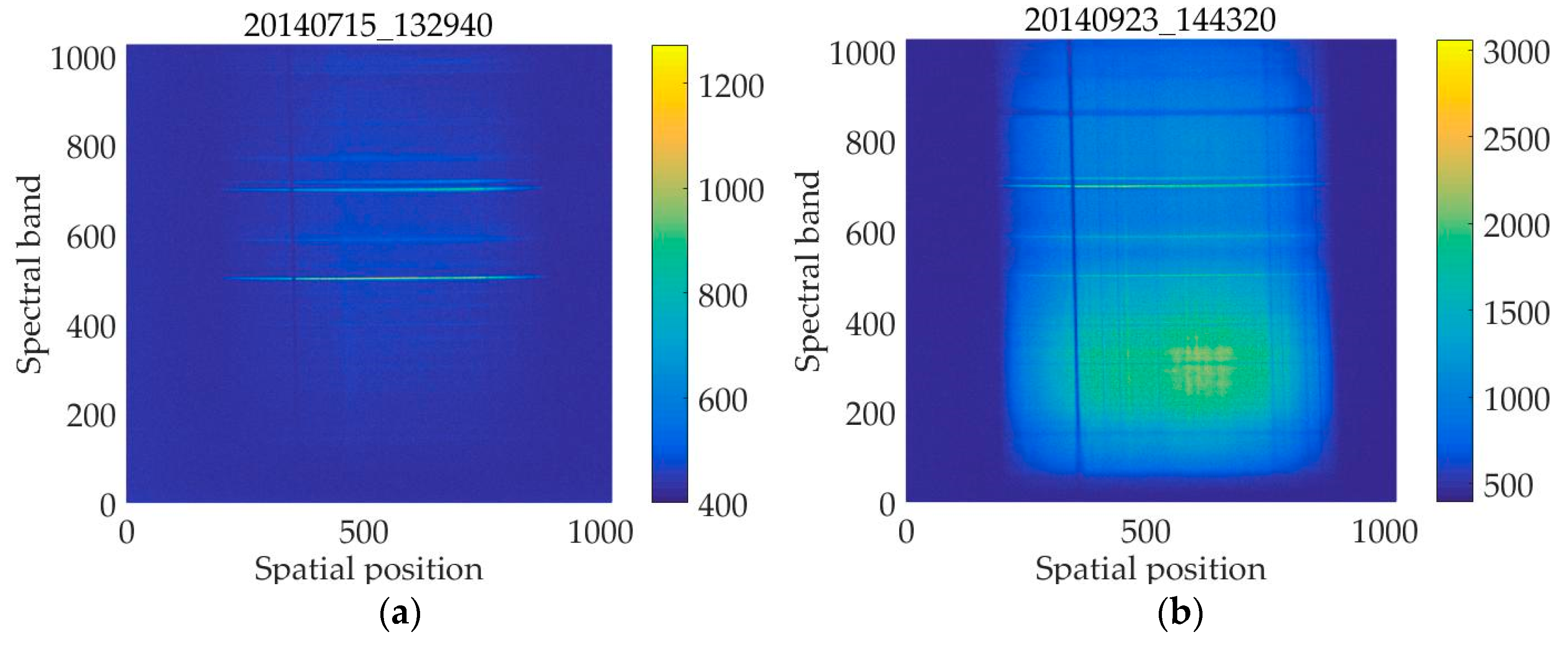
In this paper, the test dataset is the aurora spectral data collected at the Zhongshan Station in Antarctica in 2014. The temporal resolution of the camera is 15 s, i.e., an aurora spectral image is produced every 15 s. Each aurora spectral image is stored in Flexible Image Transport System (FITS) format [3] and is 1024 × 1024 in size. Each pixel is stored as a 16-bit unsigned integer. Figure 1a is an aurora spectral image captured at the Zhongshan Station on July 15, 2014, at 13:29:40, and is named as 20140715_132940. Figure 1b is an aurora spectral image captured on September 23, 2014, at 14:43:20, and is named as 20140923_144320. All the aurora spectral images referred to in the following contents will adopt this naming method. Since an aurora spectral image is produced every 15 s, the compression time must be within 15 s. Our scheme compresses the aurora spectral data using the online Differential Pulse Code Modulation (DPCM) method, and accelerate the algorithm on graphics processing units (GPUs) using Compute Unified Device Architecture (CUDA).
The idea of DPCM is to decorrelate data with linear regression prediction. Aiazzi et al. proposed two different linear regression prediction-based near-lossless and lossless still image compression algorithms. One is denoted as Relaxation-Labelled Prediction (RLP) [4], which partitions an image into small blocks and then calculates a linear predictor for each block. The other is named Fuzzy logic-based Matching Pursuit (FMP) [5], which computes the linear regression predictor through fuzzy-logic techniques. In addition, Aiazzi et al. proposed a context-based near-lossless or lossless coding method [6] for any causal DPCM scheme, which partitions prediction errors into homogeneous classes before arithmetic coding. Then, Mielikainen and Toivanen proposed a method named Clustered DPCM (C-DPCM) [7] for the lossless compression of hyperspectral images. The C-DPCM algorithm first clusters all of the spectral lines in a hyperspectral image into several classes, then computes the prediction coefficients of each spectral band of each class using the least square method (LSM), then calculates the residuals, and finally encodes the prediction coefficients and the residuals using the range coder [8]. The range coder is similar to the arithmetic coder, but is almost twice as fast as arithmetic coder.
Since both hyperspectral and aurora spectral images are spectral data, we apply the idea of DPCM to the lossless compression of aurora spectral images as well. However, an aurora spectral image has 1024 spectral bands, which is much more than the 220 or 224 spectral bands of the hyperspectral images introduced in a previous study [7], thus the total bitrate will be very large if the prediction coefficients of each band are encoded. To tackle this problem, the idea of online compression [9] is adopted in this paper. The main idea of online compression is to predict the current pixel using the already coded pixels, so that the decoder can calculate the prediction coefficients of the current pixel using the already decoded pixels, and there is no need to encode the prediction coefficients and transmit them to the decoder. Consequently, when using the online DPCM for the compression of the aurora spectral data, the only data that needs to be encoded and transmitted to the decoder is the residual. In addition, we proposed two improvements to improve the compression performance of the original online DPCM method [9]: one is on the establishment of the linear system of equations when computing the prediction coefficients, and the other is on the encoding of the residual.
In addition to DPCM, there are many other lossless compression algorithms, such as JPEG-LS (JPEG is the acronym for Joint Photographic Experts Group, and the JPEG-LS is the new standard for lossless and near-lossless compression of continuous-tone images), JPEG2000 (JPEG2000 is the successor of the JPEG with superior compression performance), and CALIC (Context-based, Adaptive, Lossless Image Codec). The core algorithm of JPEG-LS is LOw COmplexity LOssless COmpression for Images (LOCO-I) [10,11], in which a fixed predictor is used to detect vertical or horizontal edges, and the predicted value of a pixel can be seen as the median of the three candidate predicted values. JPEG2000 [12] is a wavelet-based still image compression standard, which can achieve both lossy and lossless compression within a common framework. The CALIC [13] uses a large number of modeling contexts to condition a nonlinear predictor, and the nonlinear predictor can adapt itself by learning from its past errors in a given context. However, JPEG-LS, JPEG2000, and CALIC were developed for common images, rather than spectral data.
Besides the two-dimensional (2-D) compression methods introduced above, there are also some three-dimensional (3-D) methods. Kim and Pearlman proposed the 3D-SPIHT (Three-Dimensional Set Partitioning In Hierarchical Trees) [14] for lossy video coding. Lucas et al. [15] proposed a method called 3D-MRP (Three-Dimensional Minimum Rate Predictors) for the lossless compression of medical images. Xiaolin and Memon extended the original CALIC to 3-D [16] for the lossless compression of multispectral images. Since hyperspectral images are usually very large and have high application value, many researchers have devoted their efforts to the compression of hyperspectral images using 3-D methods [17,18,19,20]. In fact, aurora spectral images can also be considered as 3-D images if the time dimension is added, and the 3-D methods can also be applied to the compression of aurora spectral images. However, the Antarctic Zhongshan Station is far from our country China and the transmission link is very limited [9], and larger files are more likely to cause transmission errors, therefore, aurora spectral images are usually compressed and transmitted frame by frame [2].
To speed up the online DPCM algorithm, this paper will take advantage of the powerful computing capability of the GPU. Traditionally, the GPU is only responsible for graphic rendering, and most of the processing is done by the central processing unit (CPU). Driven by the demand of the video game market and military scene simulation, GPU performance has rapidly improved, and now GPUs have developed into General Purpose GPUs (GPGPU). This also benefited from the development of CUDA, which is a general-purpose parallel computing platform and programming model, and allows programmers to program with the high-level programming language C. GPUs play a significant role in the fields of finance, petroleum, astronomy, signal processing, image processing, video compression, and others.
GPUs are specialized for high arithmetic intensity, high parallelism tasks. In our online DPCM aurora spectral data compression scheme, the computing of the predicted value of each pixel is independent, so that they can be calculated in parallel using GPUs. Furthermore, the prediction coefficients for each pixel are calculated using the least square method (LSM), and the main operations of LSM are matrix multiplication and matrix inversion, both of which are well-suited for acceleration with GPUs. Therefore, it is reasonable and suitable to accelerate the online DPCM algorithm in parallel with GPUs. Many researchers have utilized GPUs to speed up their algorithms. Simek and Asn [21] and Tenllado et al. [22] introduced parallel implementations of the 2-D Discrete Wavelet Transform (2D-DWT) on GPUs. The wavelet-based still image compression standard JPEG2000 was implemented on GPUs in a previous study [23]. Santos et al. [24] and Keymeulen et al. [25] used GPUs to speed up lossy and a lossless hyperspectral image compression algorithms, respectively. Wu et al. [26] implemented a GPU-based spatially adaptive hyperspectral image classification method.
The rest of the paper is structured as follows. Section 2 introduces the online DPCM method for aurora spectral data compression. Section 3 presents the detailed CUDA implementation of the online DPCM method. Section 4 analyzes the performance of the serial and the CUDA parallel implementations of the online DPCM algorithm, and optimizes the CUDA implementation using multi-stream and multi-GPU techniques, respectively. Finally, Section 5 summarizes this paper.
2. The Improved Online DPCM Method for Aurora Spectral Data Compression
2.1. Overview of the Online DPCM Method
The main steps of the online DPCM algorithm for aurora spectral image compression are as follows:
- Compute the prediction coefficients for each pixel;
- Calculate the prediction image and its difference from the original image, i.e., the residual;
- Encode the residual.
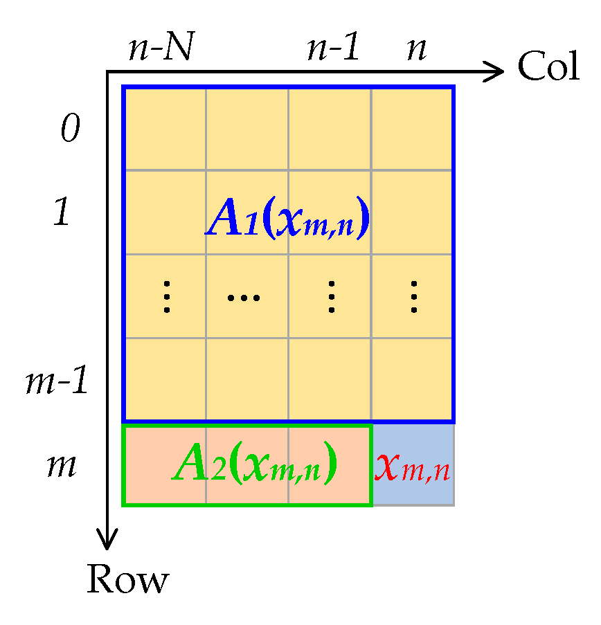
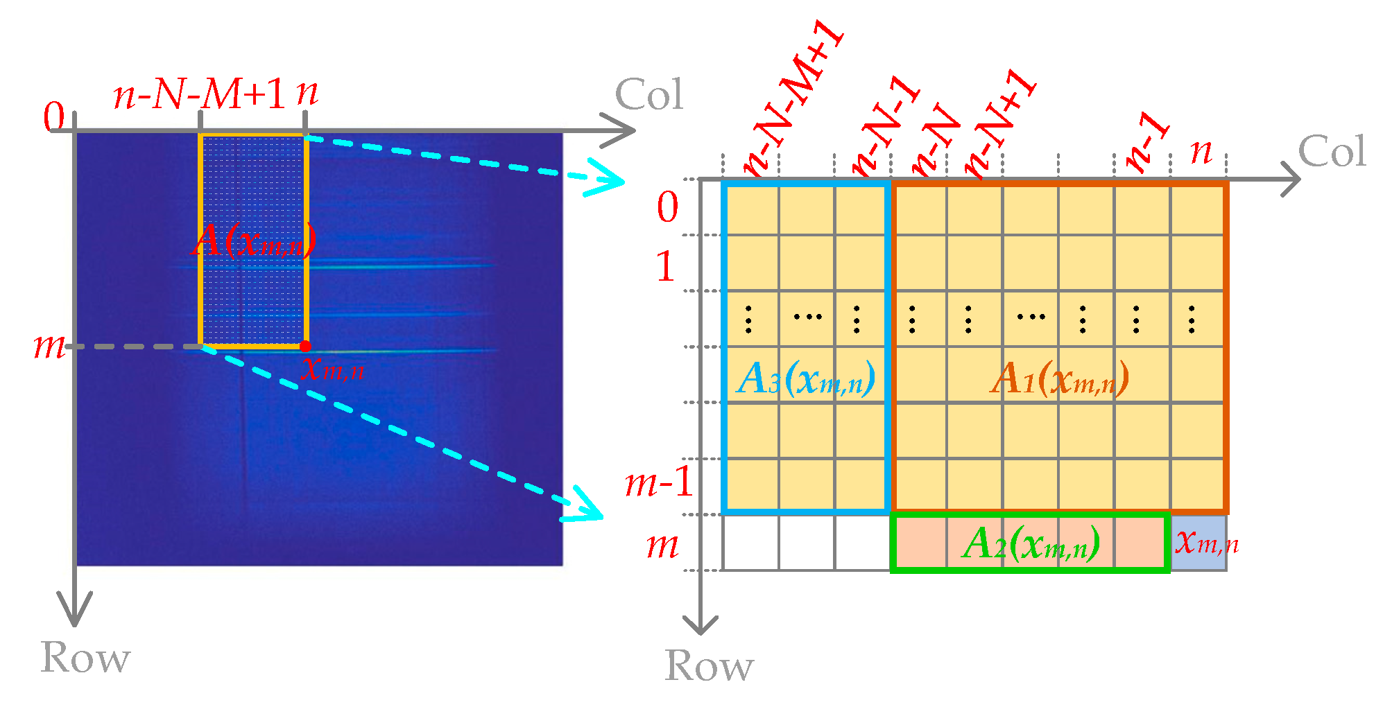
The prediction coefficients are calculated using the least square method (LSM). Figure 2 shows a pixel xm,n and the area used to predict it, and Equation (1) is the linear system of equations built to compute the prediction coefficients for xm,n. N is the prediction order, which defines how many previous columns were used to compute the prediction coefficients. The is the pixel at the ith row and the jth column, and is the prediction coefficient vector. It can be seen that the linear system of the equations involves all the pixels in area A1(xm,n), but does not involve the xm,n itself. Therefore, the decoder can also compute the prediction coefficients of xm,n using the pixels in A1(xm,n), and there is no need to transmit the prediction coefficients to the decoder. This is the idea of online compression.
Then, if we denote the first matrix in Equation (1) as C, denote the vector as , and denote the vector on the right of the equal sign as , we get the condensed format of Equation (1), that is, , and finally the coefficient vector can be computed using Equation (2) [2].
From Equation (2), the calculation of the prediction coefficients requires one matrix multiplication, one matrix inversion, and two matrix-vector multiplications (), and the calculation of the prediction coefficients is actually the most time-consuming part in DPCM. The computation of the predicted value of a pixel is much simpler, for example, the predicted value of the pixel xm,n in Figure 2 is the linear combination of the pixels in the area A2(xm,n). We use Equation (3) to describe this; is the predicted value of xm,n.
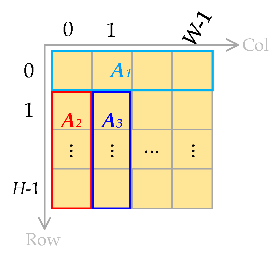
However, we cannot compute the predicted values for some edge pixels of an aurora image using Equation (3), such as the three regions A1, A2, and A3 shown in Figure 3, which is because we cannot build a linear system of equations, such as Equation (1), to compute the prediction coefficients for these edge pixels. In Figure 3, the H is the height of an aurora image, and W is the width, A1 is the row 0, and A2 is the column 0. Since there is no row before row 0 and no column before column 0, A1 and A2 cannot be predicted using LSM. A3 is column 1, since there is only one column before column 1; in other words, there is only one item on the left of the equal sign if we build a linear system of equations, and we will not predict A3 using the LSM. Equation (4) shows the prediction method for each area. The is the predicted value of xm,n. In A1 and A3, the predicted value of each pixel is the value of the adjacent pixel in the column direction, except the pixel x0,0. In A2, the predicted value of each pixel is the value of the adjacent pixel in the row direction.
The residual is the difference between the original value and the predicted value. The encode method is the range coder [8]. Since we are using the online DPCM method, the only data that needs to be encoded and transmitted to the decoder is the residual.
2.2. Our Improvement to the Original Online DPCM Method
Through experiments we found that the compression performance of the online DPCM algorithm can be improved by two improvements. One is on the establishment of the linear system of equations when computing the prediction coefficients, and the other is on the encoding of the residual.
2.2.1. The Improvement on the Establishment of the Linear System of Equations
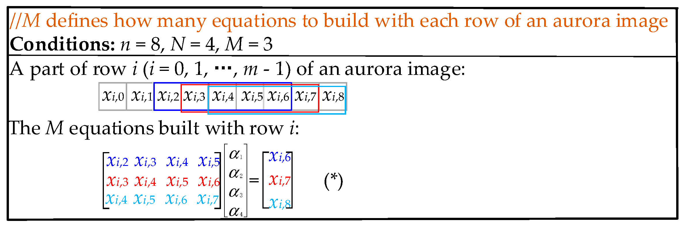
From Equation (1), only one equation is built with each of the previous rows of pixel xm,n, but through experiments we found that the compression performance can be improved when building multiple equations with each of the previous rows. We use the example shown in Figure 4 to illustrate how to build multiple equations with each row of an aurora image; xm,n is the pixel for which we are to compute its prediction coefficients. M is the number of equations built with each of the previous rows of xm,n. Suppose M = 3, the prediction order N = 4, and the column number n = 8, then the M equations built with row i (i = 0, 1, …, m − 1) are (*), shown in Figure 4. It is worth noting that these equations can be obtained when sliding a window of length N + 1 on a row.
Combining the equations built with each of the rows before the pixel xm,n, we get the complete linear system of equations used to compute the prediction coefficients of xm,n, and the linear system of equations is shown in Equation (5). The M equations in the red dashed box are built with one row of the aurora image. It can be seen that each red dashed box contains N + M different elements of a row of the aurora image, in other words, continuous N + M elements in each of the rows before row m will be used to compute the prediction coefficients of the xm,n. Figure 5 is used to explain this more clearly. Compared with Figure 2, the improved method requires more area, that is, A3(xm,n), whose number of columns is M − 1, and the total number of columns of A1(xm,n) and A3(xm,n) is N + M. Since Equation (5) is the improvement to Equation (1), we denote Equation (5) as as well, and C, and , which will be mentioned in the following contents, are the C, , and in Equation (5). Note that the number of columns of matrix C is the prediction order N, and the number of rows of matrix C is M × m, which varies with the row number m.
![Remotesensing 11 01635 i001]()

2.2.2. The Improvement on the Encoding of the Residual
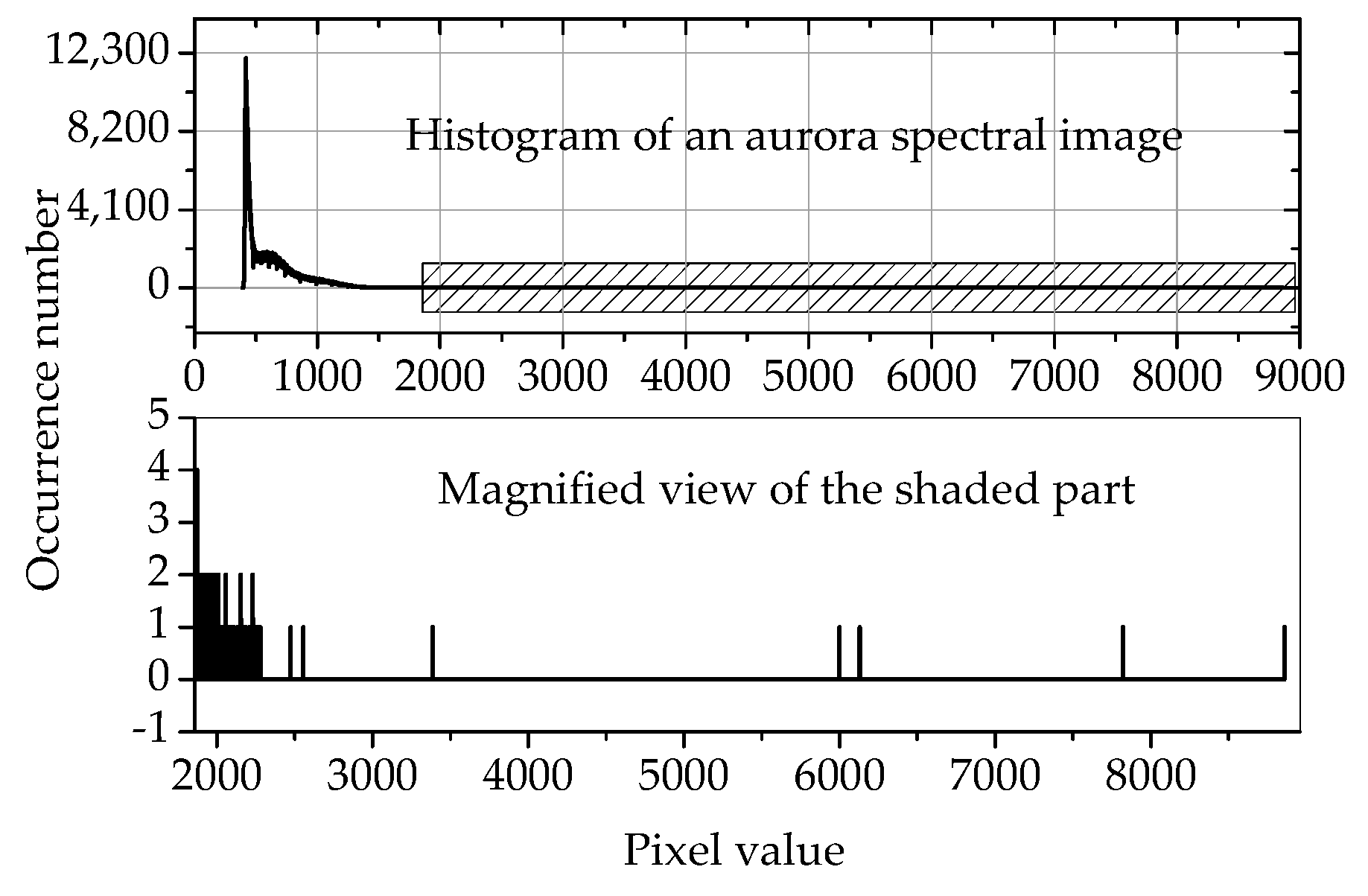
In this paper, the data to be compressed is the aurora spectral data captured at the Zhongshan Station in 2014, but we found that it had a shortcoming that would adversely affect the compression. Each aurora spectral image had some outliers that were much larger than other pixels, but only appear several times, as shown in Figure 6. These outliers are difficult to predict, consequently introducing very large residuals that have detrimental effects on compression. To handle this problem, we propose a dual threshold method that sets a threshold for positive and negative residuals, respectively. Only the residuals between the two thresholds will be encoded using the range coder, and other residuals will be stored intact in the compressed file.
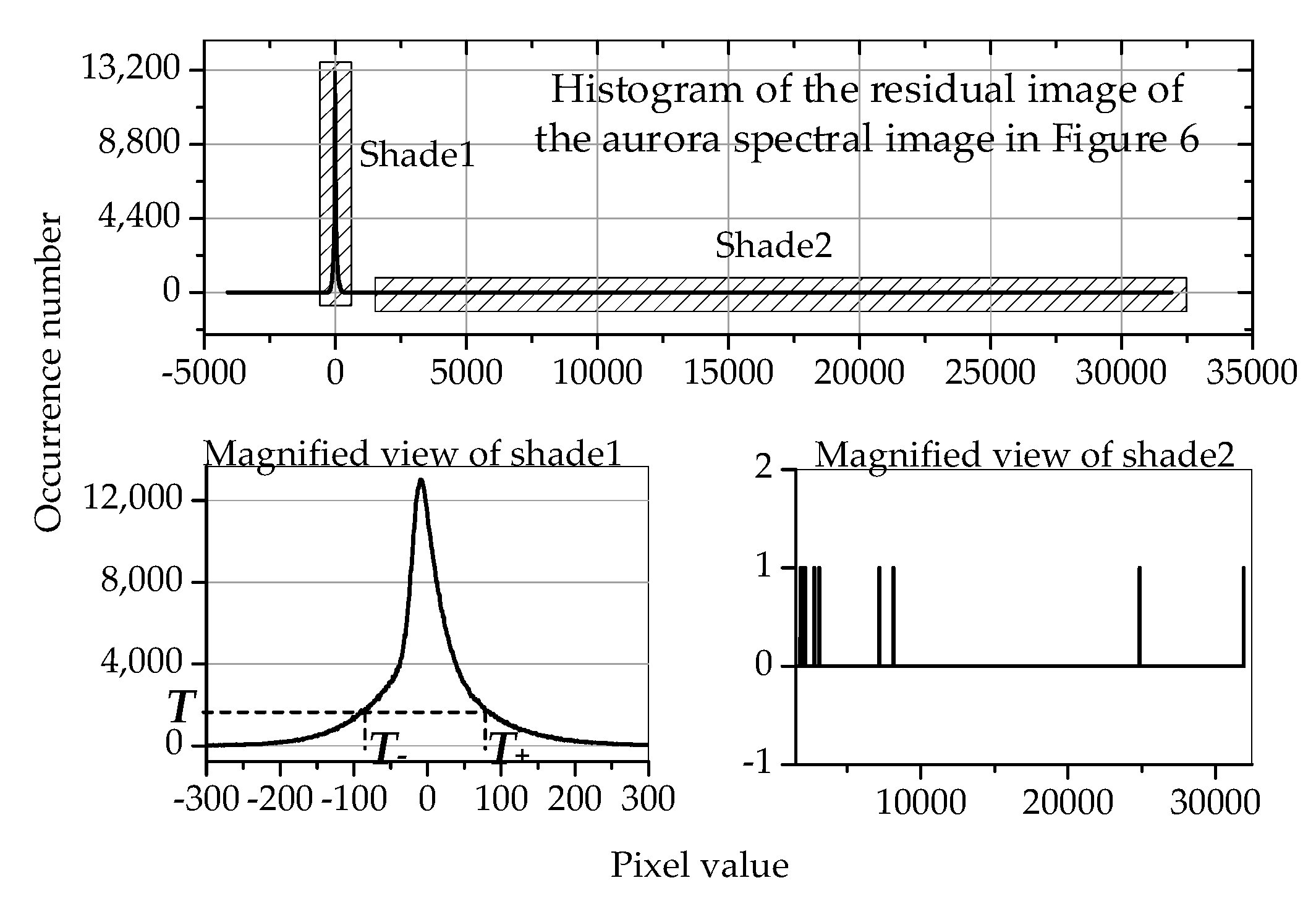
Figure 7 shows the details of the dual threshold method. The T is a threshold for the occurrence number of the residuals. T− is the first residual whose occurrence number is larger than or equal to T when searching from left to right, and T+ is the first residual whose occurrence number is larger than or equal to T when searching from right to left. Only the residuals between T− and T+ will be encoded using the range coder, and the remaining residuals will be stored intact in the compressed file.
2.3. Optimization of the Parameters N, M, and T
The parameter N determines how many columns to use to predict the current pixel and M defines how many equations to build with each row of an aurora spectral image. Both of these parameters have important impacts on the accuracy of the prediction. The threshold T determines the two thresholds T− and T+, which will affect the encoding. In order to get the best compression performance, we must optimize these parameters N, M, and T through experiments. The experimental data set is the 2014 aurora spectral data set. Since aurora does not appear every day, the 2014 aurora spectral data set has more than 20 days of data, and each day has hundreds of images. In order to reduce the amount of calculations, we evenly take 100 samples from the images of each day for experiments.
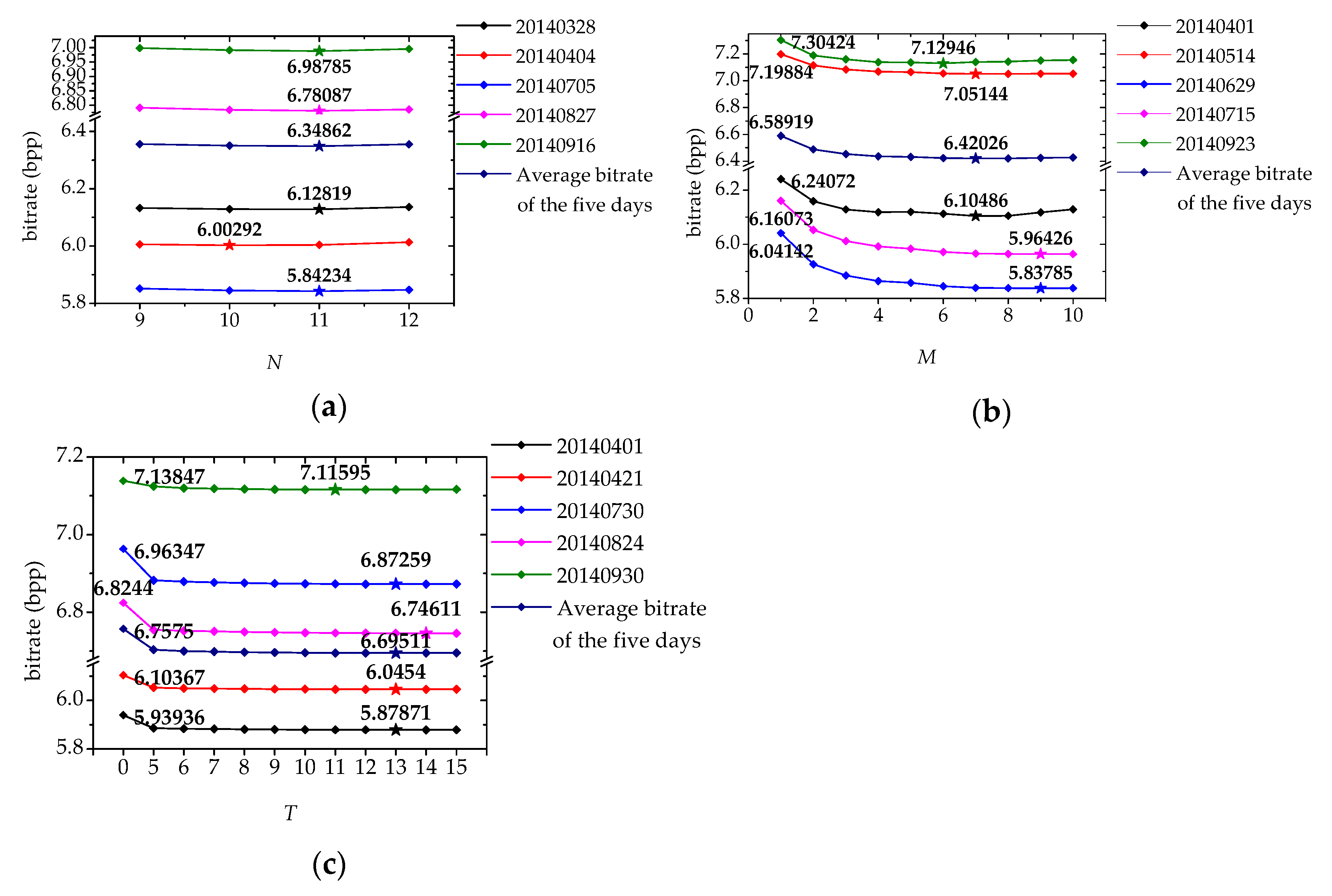
Figure 8a presents the variation of the bitrate with the prediction order N. The bitrate is the average bitrate of 100 samples evenly selected from the data of each day and is measured in bpp (bits per pixel). The four values on the horizontal ordinate, 9, 10, 11, and 12, are determined by preliminary experiments. The five-pointed star symbol on each line indicates the optimal N that minimizes the average bitrate of each day, and the number near the five-pointed star symbol is the minimum bitrate. It can be seen that the optimal N for four days is 11, and for one day is 10. In order to determine the final N that minimizes the average bitrate of each day, we averaged the bitrate of the five days, and the result is the third line from top to bottom in Figure 8a. We can see that N = 11 minimizes the average bitrate of the five days, and therefore, we take N = 11 as the prediction order for the 2014 aurora spectral data compression.
Figure 8b is similar to Figure 8a, but shows the variation of the bitrate with M, which defines how many equations to build with each row of an aurora spectral image. There are 10 values for M, 1, 2, …, 10. It can be seen that the optimal M that minimizes the bitrate of each day is different, but the M that minimizes the average bitrate of the five days is 7. Therefore, we take M = 7 for the compression of the 2014 aurora spectral data.
Note that the bitrate of each day when M = 1 is also presented near the first diamond node on each line in Figure 8b. The difference between the minimum bitrate and the bitrate when M = 1 ranges from more than 0.1 bpp to more than 0.2 bpp, and the average bitrate of the five days when M = 1 is about 0.17 bpp more than the minimum average bitrate of the five days. Consequently, we can conclude that the improvement to build multiple equations on each row of an aurora spectral image is beneficial to compression.
Figure 8c shows the variation of the bitrate with T, which determines the two encoding thresholds T− and T+. There are 12 values on the horizontal ordinate, 0, 5, 6, …, 15. T = 0 represents that there are no thresholds and all the residuals will be encoded using the range coder. It can be seen that the optimal T that minimizes the bitrate of each day is different, but the minimum of the average bitrate of the five days is achieved when T is 13. Therefore, we will choose T = 13 for the compression of the 2014 aurora spectral data. In addition, the bitrate of each day at T = 0 is shown near the first diamond node on each line. We can see that the bitrate at T = 0 is larger than the minimum bitrate on each line, and the average bitrate of the five days when T = 0 is about 0.06 bpp more than the minimum average bitrate of the five days. Therefore, the dual threshold method for encoding is effective.
3. The GPU Implementation of the Calculation of the Prediction Coefficients using the Improved Online DPCM Algorithm
The most time-consuming part of the online DPCM algorithm is the calculation of the prediction coefficients, which is because the prediction coefficients for each pixel are obtained by solving a linear system of equations. In addition, since this is an online method, the decoder also needs to compute the prediction coefficients for each pixel. Therefore, the calculation of the prediction coefficients must be accelerated, and this paper takes advantage of the powerful computing capability of GPUs.
From Equation (2), the main operations in the calculation of the prediction coefficients are matrix multiplication and matrix inversion. Hence, the rest of this section will focus on these two steps, but before that, we will introduce some basic concepts of GPU programming to facilitate the following descriptions.
3.1. Some Basic Concepts of GPU Programming
GPU is specialized for computation-intensive tasks. The programming model of GPU is CUDA, and the programming language is CUDA C. The kernel functions, which are much like the C functions but run on GPU, are labelled by hundreds of thousands of CUDA threads in parallel to handle the massive computations, and NVIDIA (a GPU corporation) denotes this architecture as Single Instruction Multiple Thread (SIMT).
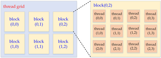
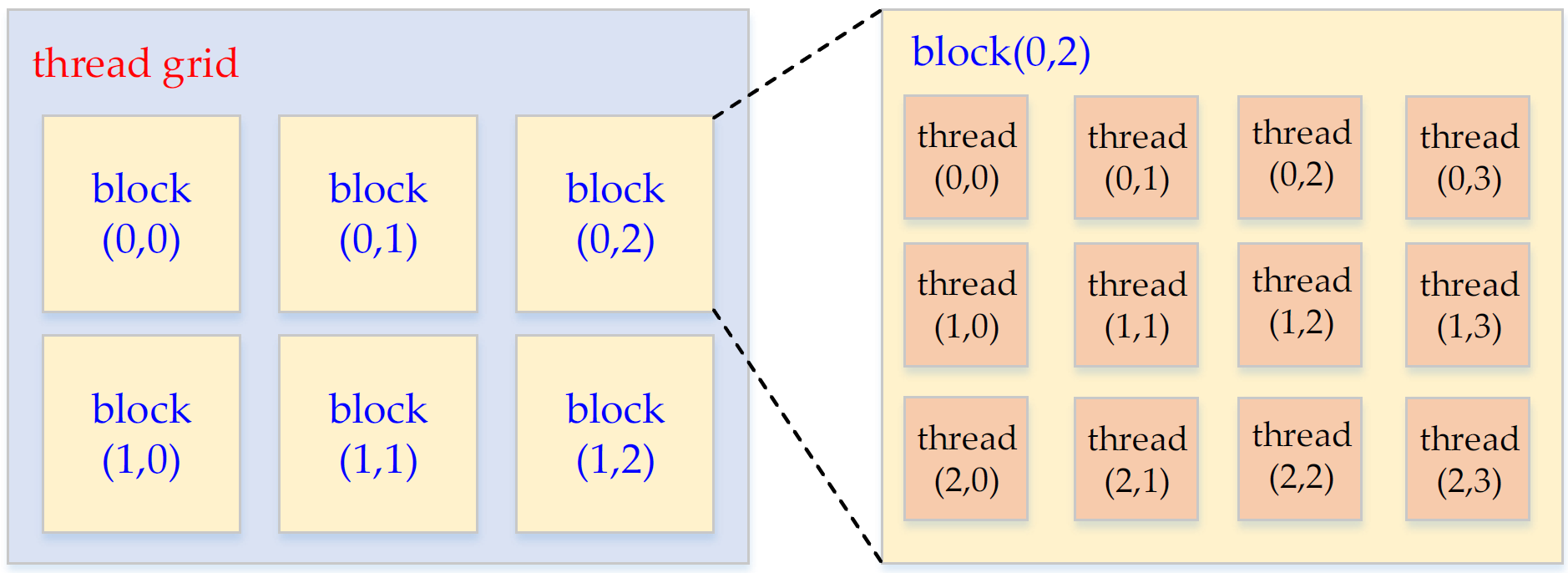
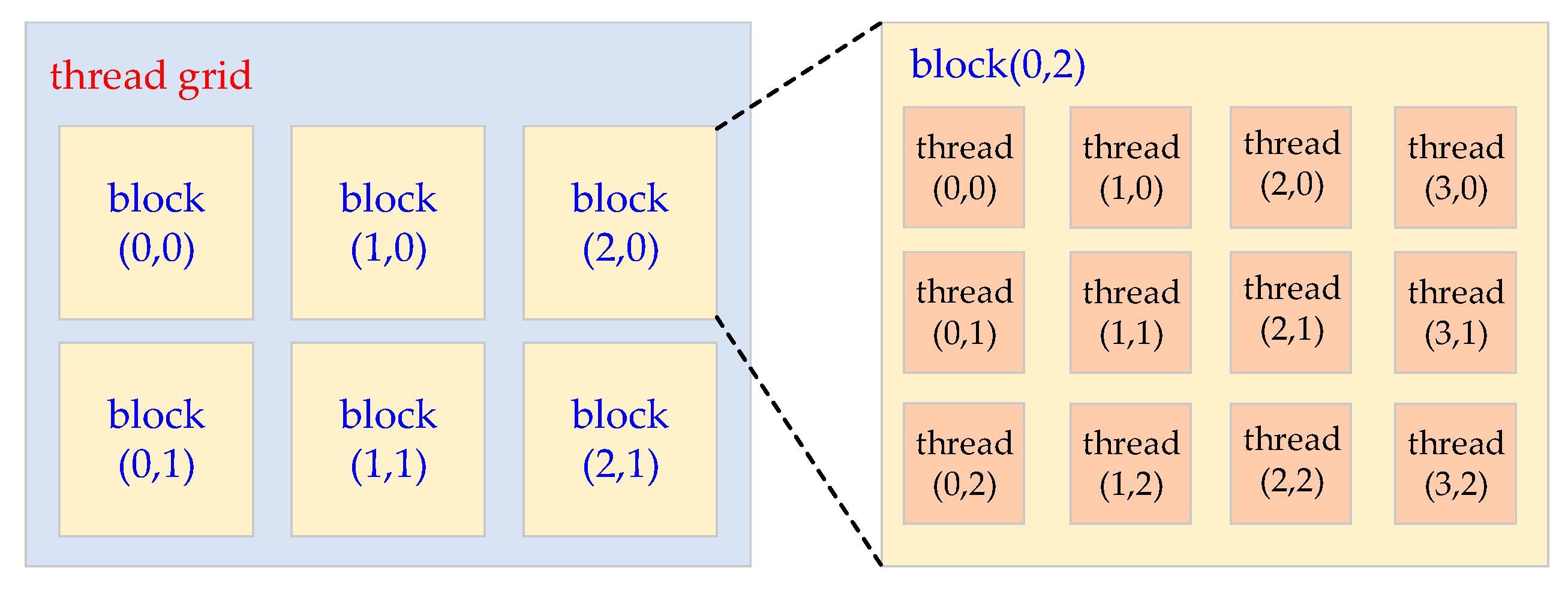
All the threads assigned to a kernel function are organized into a two-hierarchical grid structure. A number of threads form a thread block, and a number of thread blocks form a thread grid. The size of all the thread blocks in a thread grid is the same. Both a thread block and a thread grid can be one-dimensional, two-dimensional, or three-dimensional. Figure 9 presents an example describing the thread structure. The size of the thread grid is 3 × 2, and the size of each thread block is 4 × 3. The ordered pair in parentheses is the index of a thread or a thread block.
The typical processing flow of a CUDA program is: (1) copy the data to be processed from host (the CPU memory) to device (the GPU memory); (2) launch the kernel function to process the data on the GPU; (3) copy the result from device to host. In addition, there is a type of memory that is very critical to the performance of a CUDA program—shared memory. Shared memory is on-chip memory, and its access latency is only a few clock cycles, which is much less than the access latency of the hundreds of clock cycles of global memory. Furthermore, shared memory provides a means of communication for all of the threads in a thread block.
3.2. CUDA Implementation of the Multiplication of Matrices CT and C using a Decomposition Method
Matrix multiplication is a common operation in CUDA programming, and has been optimized very well. The Basic Linear Algebra Subprogram (cuBLAS) [27] is a linear algebra acceleration library for CUDA, which can process not only the matrix multiplication but also the matrix multiplication of a batch of matrices. In our case, the multiplication of matrices CT and C in Equation (2) is required to predict each pixel, and there are 1024 × 1024 pixels in each aurora spectral image. However, the multiplication of matrices CT and C cannot be batch processed using the cuBLAS library, which is because the size of matrix C is not fixed; it is determined by the row number of the pixel to be predicted, as shown in Equation (5), and the cuBLAS library can only process a batch of matrices with the same dimensions. In addition, if the multiplication of matrices CT and C for each pixel is performed individually using the cuBLAS matrix multiplication function, the launch overhead is too heavy. Therefore, the cuBLAS library is not adopted for the multiplication of matrices CT and C, and we must propose a scheme that is suitable for the situation in this paper.
From Equation (5), when predicting a pixel xm,n at the mth row and the nth column, all the rows before row m will be involved in its matrix C; let us label the matrix C as C(xm,n) for the simplicity of description. Similarly, all of the rows before row m + 1 will be involved in matrix C(xm+1,n) when predicting xm+1,n. Furthermore, the first m × M row in matrix C(xm+1,n) is exactly the matrix C(xm,n), so if the multiplication of matrix CT(xm,n) (the transposed matrices of C(xm,n)) and C(xm,n) and the multiplication of matrices CT(xm+1,n) and C(xm+1,n) are performed directly and individually, many repeated data access instances and calculations will be introduced, which will seriously affect the computational efficiency. Therefore, we proposed a decomposition method for the multiplication of matrix CT and C to handle this problem.
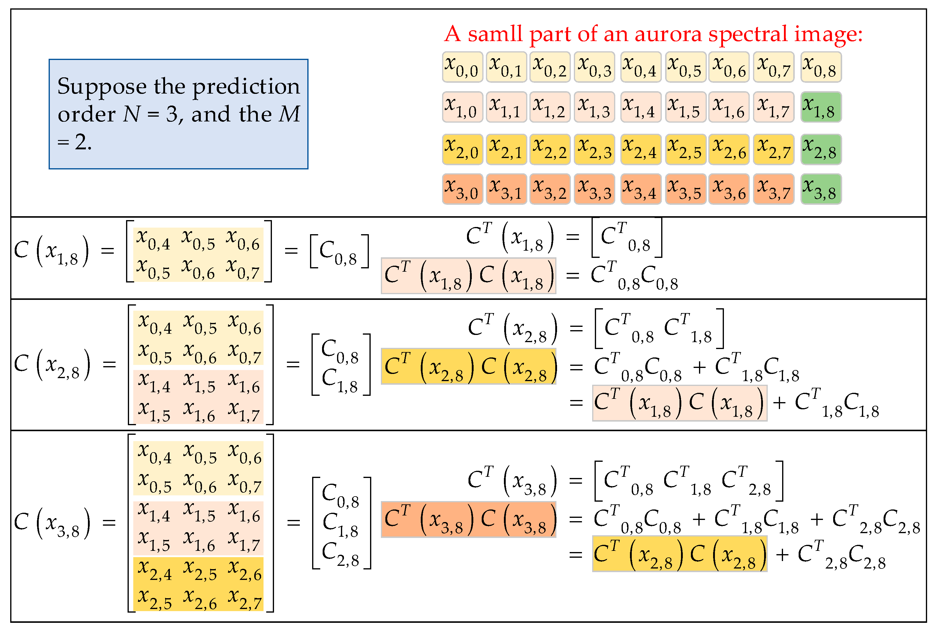
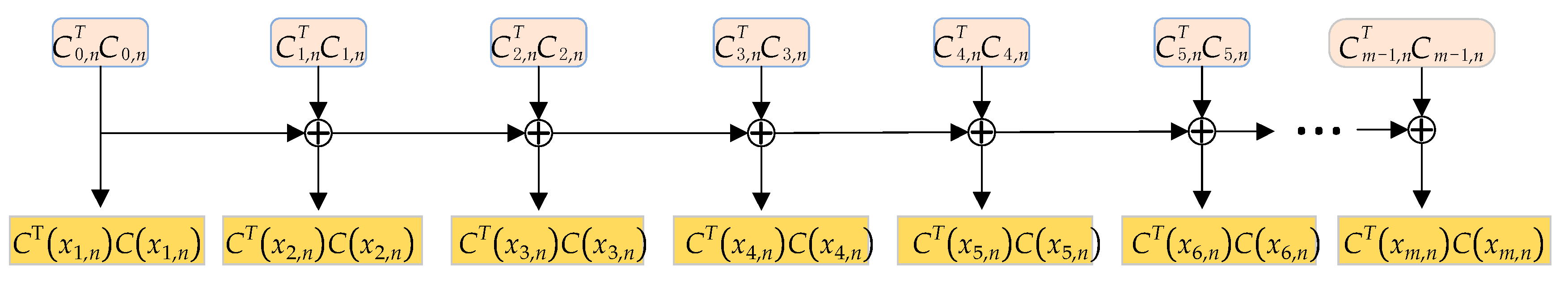
Figure 10 shows an example illustrating the decomposition method for the multiplication of matrices CT and C. A small part of the upper left corner of an aurora spectral image is shown in the upper right corner of Figure 10. For simplicity, we assume that N = 3 and M = 2, and that we are to predict three pixels, x1,8, x2,8, and x3,8. C(x1,8), C(x2,8), and C(x3,8) represent matrix C for the three pixels x1,8, x2,8, and x3,8, respectively, and CT(x1,8), CT(x2,8), and CT(x3,8) are the transposed matrices for C(x1,8), C(x2,8), and C(x3,8), respectively. The two rows of matrix C(x1,8) are grouped together and denoted as C0,8. The subscript “0” of C0,8 represents that the two rows are built with row 0 of the aurora image, and the subscript “8” represents that the pixel to be predicted is located in column 8. Similarly, C(x2,8) is partitioned into two submatrices C0,8 and C1,8, and C(x3,8) is partitioned into three submatrices C0,8, C1,8, and C2,8. Therefore, the product of the matrices CT(x1,8) and C(x1,8) is CT0,8C0,8; the product of CT(x2,8) and C(x2,8) is CT0,8C0,8 + CT1,8C1,8, which can also be considered as CT(x1,8)C(x1,8) + CT1,8C1,8; the product of CT(x3,8) and C(x3,8) is CT0,8C0,8 + CT1,8C1,8 + CT2,8C2,8, which can also be considered as CT(x2,8)C(x2,8) + CT2,8C2,8. It can be seen that the multiplication of matrices CT(xm,n) and C(xm,n) is transformed into the addition of many small matrices, and CT(xm,n)C(xm,n) is the sum of CT(xm−1,n)C(xm−1,n) and CTm−1,nCm−1,n. In this way, all the matrices CT(xi,n)C(xi,n) (i = 1, 2, …, m) can be obtained when the prefix sums an array of matrices, CT0,nC0,n, CT1,nC1,n, …, CTm−1,nCm−1,n. The idea of this method is intuitively presented in Figure 11.
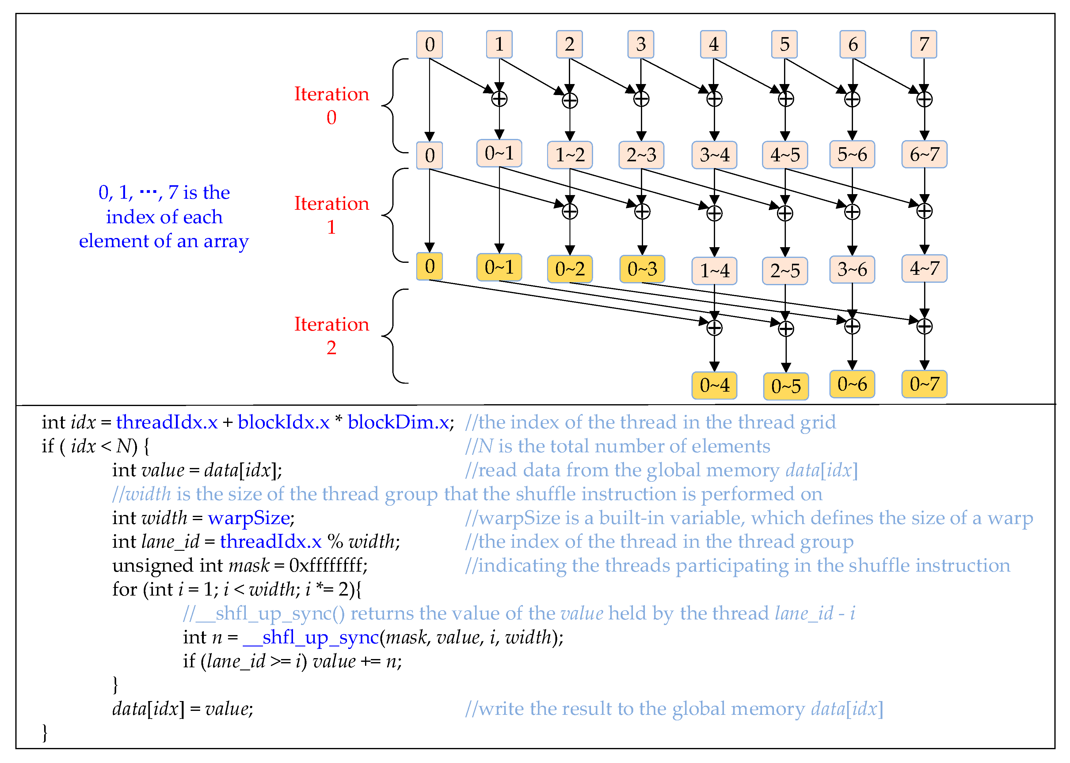
In order to accelerate the method introduced in Figure 11, a parallel scheme shown in Figure 12 is utilized in this paper. It is noteworthy that the purpose of the summation of two matrices is to add the elements in the same position. Similarly, the purpose of the prefix summing of a series of matrices is to prefix sum arrays composed of all the elements at the same position in the matrices. Therefore, the method introduced in Figure 12 is actually a parallel method for prefix summing of arrays. The upper part of Figure 12 is an example that depicts how to compute the prefix sum of an array with 8 elements. The i~j (i < j) represents the sum of the ith element to the jth element. It can be seen that the prefix summing of 8 elements is completed through 3 iterations.
The lower part of Figure 12 shows the CUDA codes for prefix summing of elements in a warp. The __shfl_up_sync() [28] is a CUDA shuffle instruction, which allows threads in the same warp to exchange data directly without consuming extra memory, and has lower latency than shared memory. This is why we use __shfl_up_sync(). The maximum range of action of __shfl_up_sync() is an entire warp, but in fact a warp can be evenly divided into a few thread groups, and __shfl_up_sync() is executed on each thread group individually. The width in the CUDA codes in Figure 12 is exactly the size of each thread group, and it is set to warpSize, which is 32. The function of __shfl_up_sync (mask, value, i, width) is to get the value of the value of the thread lane_id − i. It can be seen that the main body of the CUDA codes is a for loop. In the ith iteration, all the threads except the first i threads call __shfl_up_sync() to get the value of value held by the thread lane_id − i, and then add the obtained value to its own value. After five iterations, the prefix summing of a warp with 32 threads is completed. However, this only achieves the prefix summing in a warp; to compute the prefix sum of 1023 matrices (each aurora image has 1024 rows), we also need to compute the prefix sum inside each thread block, and finally the prefix sum across the entire thread grid.
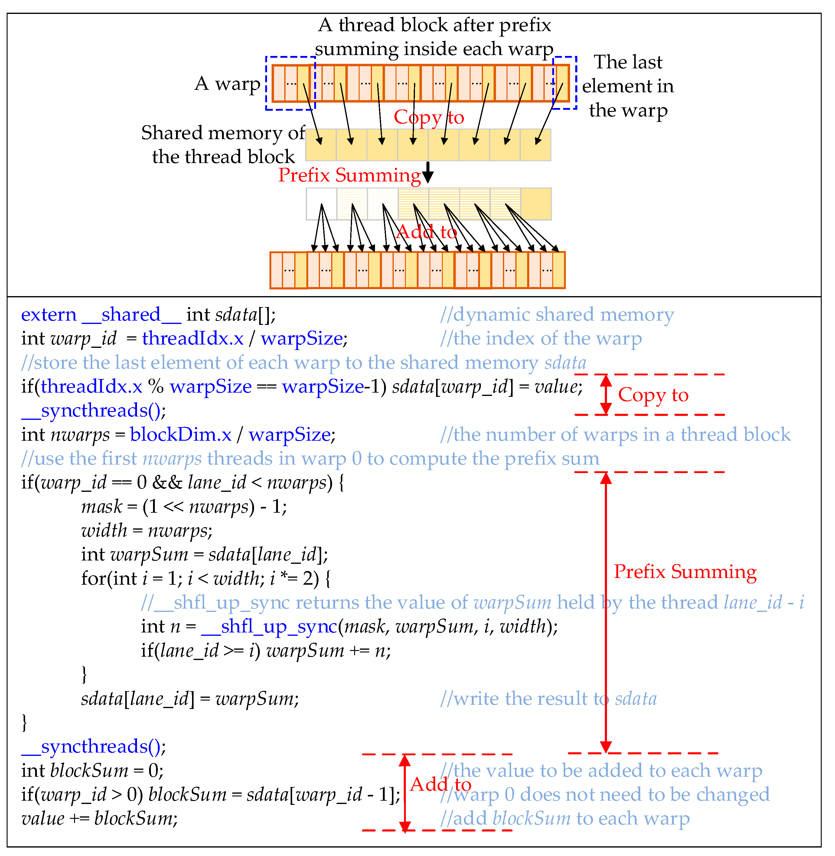
Figure 13 shows the second half of the thread block prefix summing, that is, prefix summing of the last element of all the warps in a thread block and adding each element of the resulting array to the corresponding warp. The upper part of Figure 13 depicts the general idea, and the lower part gives the CUDA codes. The codes can be divided into three parts. The first part is to copy the value, which stores the last element of each warp after the operations in Figure 12, to the shared memory sdata. The second part is to prefix sum the elements in sdata. Since there are nwarps warps in each thread block, and the last parameter width of __shfl_up_sync() is set to nwarps. The last part is to add each element of sdata to the corresponding warp. Since there is no warp before warp 0, 0 is added to warp 0.
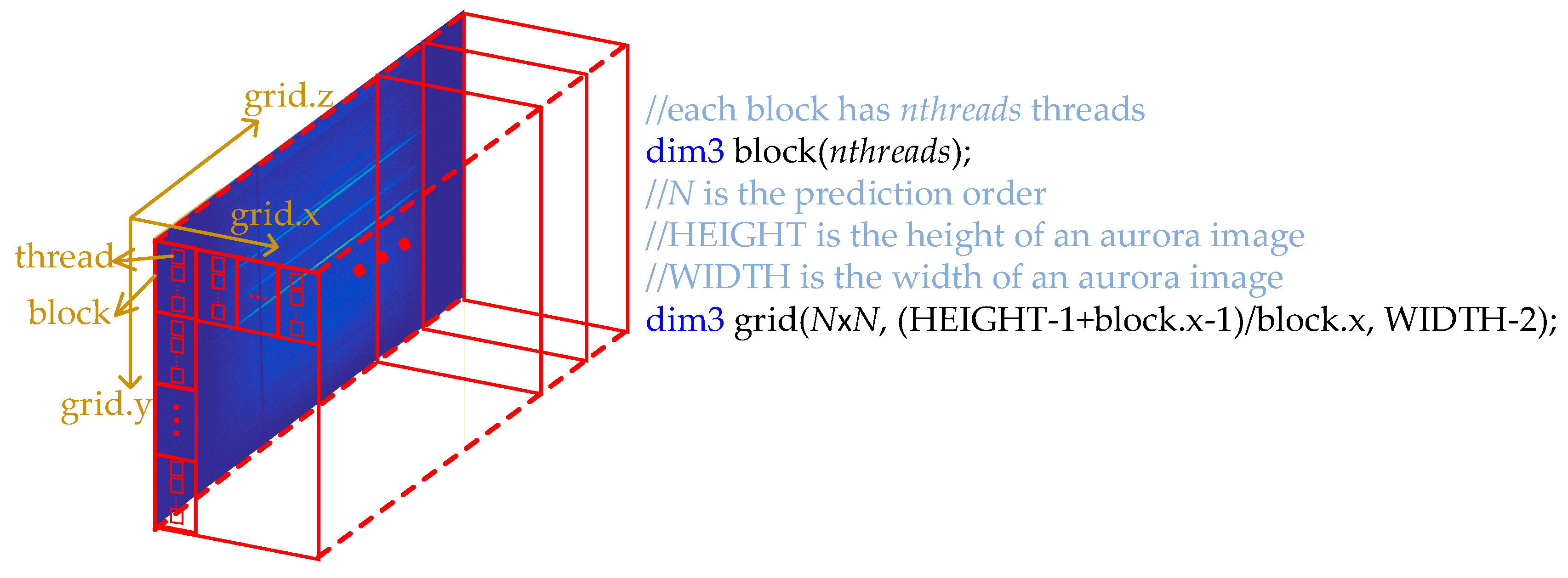
Combining the codes in Figure 12 and Figure 13, we get the CUDA kernel function for computing the prefix sum within each thread block, and denote the kernel as CTCBlockPrefixKernel. The thread structure of CTCBlockPrefixKernel is presented in Figure 14. Each page of the thread grid processes a column of an aurora image, and there are WIDTH − 2 pages in total, which is because the first two columns are predicted in advance, as illustrated in Figure 3. Suppose each thread block has nthreads threads. Since the first row of an aurora image is also predicted in advance, there are HEIGHT − 1 CTC matrices in each column of the aurora image, and the y dimension of the thread grid is (HEIGHT − 1 + block.x − 1)/block.x. Each CTC matrix has N × N (N is the prediction order) elements, so there are N × N arrays to prefix summing, and the x dimension of the thread grid is N × N.
The scheme for computing the prefix sum across a column of thread blocks of Figure 14 is similar to the method described in Figure 13. First compute the prefix sum of the last elements of each thread block, and then add each element of the resulting array to the corresponding thread block. After this procedure, we can get the matrices CT(xm,n)C(xm,n) (m = 1, 2, …, 1023, n = 2, 3, …, 1023) (the first row and the first two columns of an aurora image are predicted in advance, as illustrated in Figure 3).
The preceding contents have talked about how to decompose the CT(xm,n) × C(xm,n) into the addition of many small matrices CTi,nCi,n (i = 0, 1, …, m − 1), but the multiplication of the matrices CTi,n and Ci,n still remains a problem. From Figure 10, the size of Ci,n is M × N, M determines how many equations to build with each row of an aurora image and N is the prediction order. Therefore, the dimension of the matrix CTi,nCi,n is N × N. Furthermore, the optimal N is 11 for the 2014 aurora data set, as described in the Section 2.3, so there are 11 × 11 = 121 elements in each CTi,nCi,n, which is much less than the maximum number of threads (1024) supported by each thread block of the recent GPU cards. Consequently, a thread block is enough for the multiplication of CTi,n and Ci,n, and each thread is responsible for an element of the product matrix CTi,nCi,n. Of course, if the dimension of the matrix CTi,nCi,n is larger than the maximum number of threads supported by each thread block, the product matrix CTi,nCi,n can be divided into small submatrices and each thread block processes one submatrix, as presented in the matrix multiplication sample in a previous study [28].
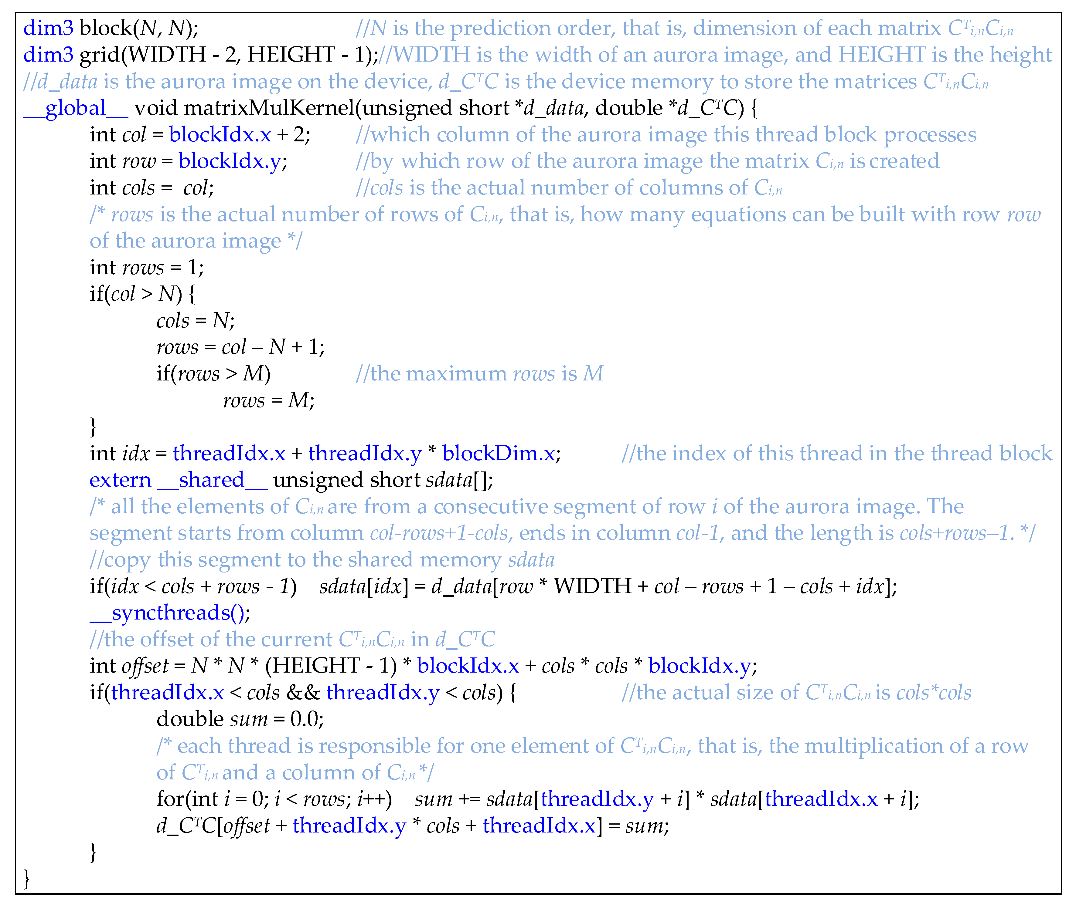
Figure 15 gives the CUDA implementation of the multiplication of matrices CTi,n and Ci,n. The size of the thread block is N × N, which is the same as the size of the product matrix CTi,nCi,n. Each thread is responsible for one element of CTi,nCi,n, in other words, each thread is responsible for the multiplication of a row of CTi,n and a column of Ci,n. The size of the thread grid is (HEIGHT − 1) × (WIDTH − 2), which is because the first row and the first two columns of an aurora image are predicted in advance. Since the first several columns of an aurora image cannot establish a matrix Ci,n with M rows and N columns, cols and rows are used to represent the actual width and height of Ci,n, respectively. If col (the index of the current column of the aurora image) is less than or equal to N, cols is col, and rows is 1, otherwise, cols is N, and rows is col − N + 1, which is the maximum number of equations can be built with each row of the aurora image, but if rows is larger than M, rows is set to M. Since all the elements of Ci,n are from a consecutive segment of row i of the aurora image, as shown in Figure 10, the segment is copied to the shared memory sdata to reduce the accesses of the global memory d_data and take advantage of the low latency of the shared memory. It is noteworthy that in this way, we do not need to prepare the matrix Ci,n in advance and copy it from host to device, and the only data that needs to be transferred from host to device is the aurora data, so a lot of time is saved.
So far, the introduction of the matrix multiplication is complete, but this decomposition idea can also be applied to the multiplication of CT and in Equation (2). This is because C(xi−1,n) is the prefix of C(xi,n), as shown in Figure 10, and (the right-hand-side vector corresponding to C(xi−1,n)) is also the prefix of .
3.3. CUDA Implementation of the Inversion of Matrix CTC using the Gaussian Jordan Elimination Method
As shown in Equation (2), the inversion of matrix CTC is one of the most important procedures when computing the prediction coefficients of a pixel of an aurora image. The method for the inversion of CTC used in this paper is the Gaussian Jordan Elimination method [29,30], and this subsection mainly talks about how to accelerate it in parallel using CUDA. The main step of the Gaussian Jordan Elimination method is to extend an identity matrix of the same dimension to the right of CTC, and then sequentially change each column of CTC into a unit vector through elimination. When matrix CTC finally becomes an identity matrix, the right half matrix is the inverse matrix. That is, , E is an N-dimensional unit matrix. In addition, it is necessary to select the main element before elimination to control the rounding error and avoid division by zero, and for convenience, the range we adopted for selecting the main element is a column.
The reason why we choose the Gaussian Jordan Elimination method is that the dimension of the matrix CTC is N, and the optimal N is 11 for the 2014 aurora spectral data set, so CTC is a medium and small-sized matrix. If we use the adjoint matrix method to compute the inverse matrix of CTC, we need to compute N × N algebraic cofactors and the determinant of CTC, which is a large amount of calculations. If we use the decomposition methods, such as LU decomposition (which decomposes a matrix into a unit Lower triangular matrix and an Upper triangular matrix) or QR decomposition (which decomposes a matrix into an orthogonal matrix and an upper triangular matrix), we first need to decompose CTC into several submatrices, then compute the inverse matrix of each submatrix, and finally compute the product of these inverse matrices. Each step of the decomposition method requires at least one call of a kernel function. Therefore, the decomposition method is very complicated and its processing time may be less than that of the Gaussian Jordan method for large matrices, but for the medium and small-sized matrix CTC, the launch overhead of the kernel functions may offset the advantage of the decomposition method.
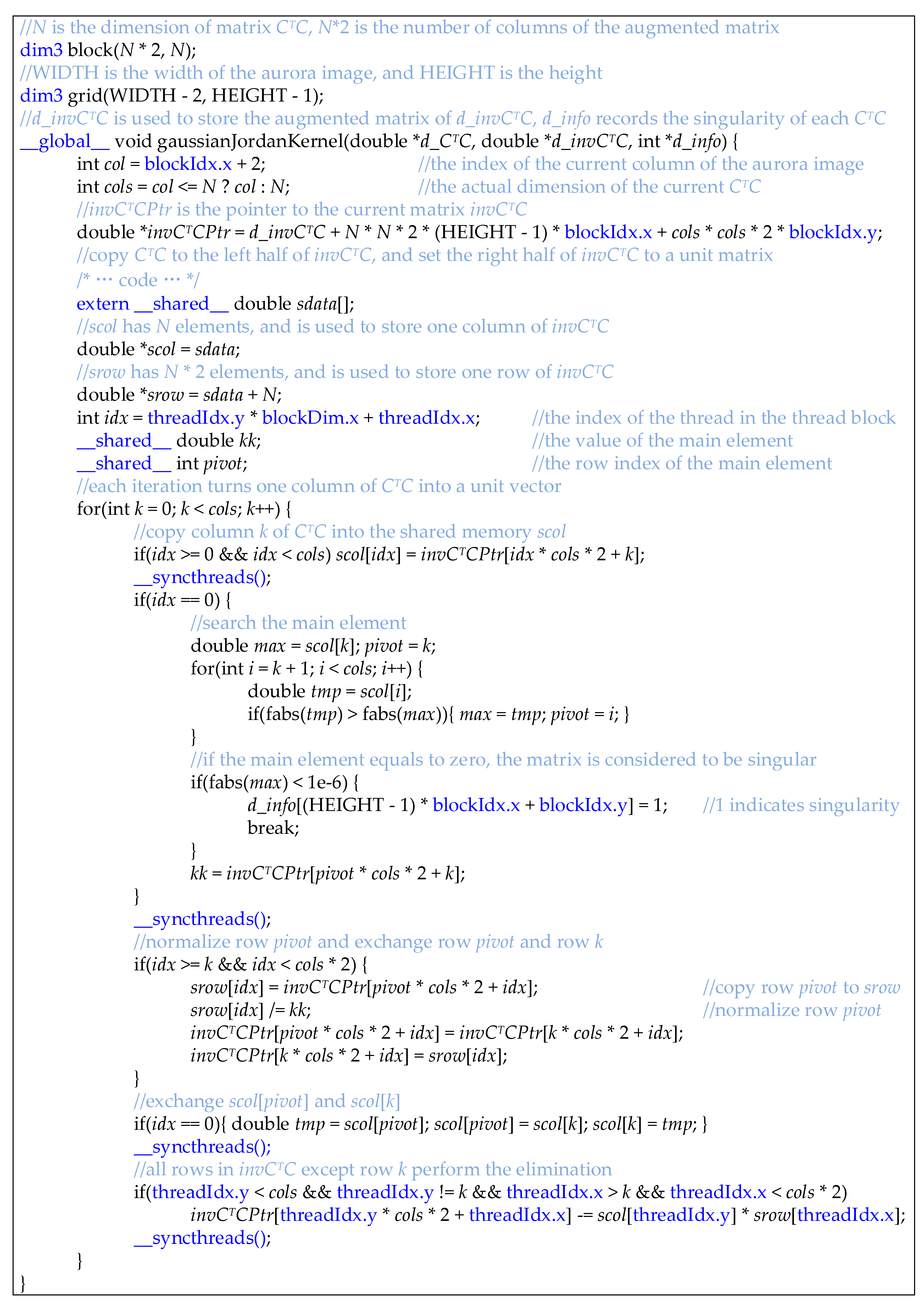
The CUDA implementation of the Gaussian Jordan method for the calculation of the inverse matrix of CTC is presented in Figure 16. Each thread block calculates the inverse matrix of a matrix CTC, and the size of the thread block is (N × 2) × N, which is the same as the size of the augmented matrix invCTC; cols is the actual dimension of the matrix CTC. First, the matrix CTC is copied to the left half of invCTC, and the right half of invCTC is set to a unit matrix. Then, each iteration of the for loop turns one column of invCTC into a unit vector through Gaussian Jordan Elimination. Since the actual number of columns of CTC is cols, there are cols iterations in the for loop. The first step in each iteration is to search the main element of a column. As there are only N = 11 elements in a column, and the search range of the main element in the kth iteration is from row k to the last row, which means that the search range of the main element is decreasing, thread 0 is assigned to search the main element in a column serially. Note that if the main element equals zero, there will be a division by zero error, and the matrix CTC is considered to be singular. The shared memory kk is used to store the main element, and the pivot is the row index of the main element. Now that the column main element has been calculated, we need to normalize the row pivot and exchange it with row k. Since the row pivot will be used several times during elimination, our scheme is to copy the row pivot to the shared memory srow to reduce the accesses of the global memory. In this way, the normalization is performed on the srow, and the row pivot and row k can be exchanged with the help of srow. The last step is elimination. Each row of the matrix invCTC, except row k, minus a certain ratio of the row pivot to turn the kth element of this row into zero. Actually, the ratio is the ratio of the kth element of each row to the kth element of row pivot. Since the row pivot has been normalized and the kth element has turned into 1, the ratio becomes the kth element of each row. It can be seen that the column k will be accessed many times during the elimination, therefore, it is copied to the shared memory scol to avoid the severe access latency of the global memory. After cols iterations, the left half of invCTC is turned into a unit matrix, and the right half is exactly the inverse matrix of CTC.
4. Experimental Results
The previous two sections have detailed the online DPCM algorithm and its CUDA implementation, and this section will focus on the verification of the performance of the CUDA implementation through experiments. The test data set is the aurora spectral data set captured at the Zhongshan Station in 2014, which is introduced in Section 1. The CPU that runs the serial program is the Intel Xeon E3-1240 v3 CPU, whose dominant frequency is 3.4 GHz. The GPU is the NVIDIA TITAN X GPU, which has 3584 CUDA cores and 12 GB GDDR5X memory, and the memory bandwidth is 480 GB/s.
4.1. The Compression Performance of the Improved online DPCM Algorithm Compared with Several Other Lossless Compression Algorithms
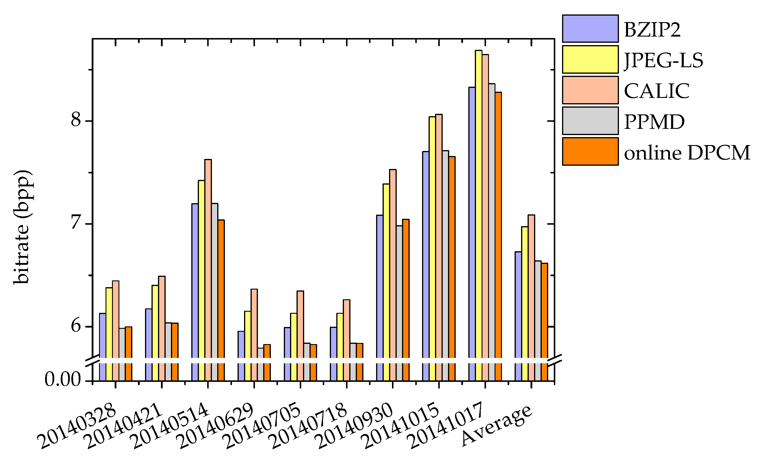
The details of the improved online DPCM algorithm are introduced in Section 2, and the three parameters N, M, and T are set to their respective optimal values, that is, N = 11, M = 7, and T = 13. Figure 17 presents the compression performance of the online DPCM algorithm and a few other lossless compression algorithms. The Bzip2 and PPMD (the Prediction by Partial Matching algorithm implemented by Dmitry)are implemented in the 7-Zip software [31]. The Bzip2 is based on the Burrows–Wheeler transform (BWT) [32] lossless data compression algorithm. The PPMD is the implementation of the PPM (Prediction by Partial Matching) with Information Inheritance (PPMII) algorithm [33] with small changes, and the PPMII is a modification of the PPM [34] algorithm to reduce its high computational complexity. The JPEG-LS [11] and the CALIC [13] are briefly introduced in Section 1. The bitrate for each day is the average bitrate of 100 aurora spectral images evenly selected from the data of each day, and the smaller the bitrate, the better the compression performance. It can be seen that the bitrate of the online DPCM is the lowest for 6 days of the 9 days, and the average bitrate of the online DPCM on these 9 days is also lower than that of all the other algorithms. Therefore, we can conclude that the online DPCM outperforms all the other algorithms shown in Figure 17.
4.2. The Performance of the Parallel Implementation of the Online DPCM Algorithm
For a CUDA program, what we are most concerned about is the speed comparison between it and its corresponding serial program. Table 1 shows the execution time for the parallel implementation and two serial implementations of the online DPCM algorithm. The time for each day is actually the average time for 100 aurora spectral images evenly selected from the data of each day. The purpose of the “serial decomposed” implementation is to apply the idea of decomposition introduced in Section 3 to the matrix multiplication CT × C and the matrix-vector multiplication CT × (as shown in Equation (2), and the purpose of the “serial direct” implementation is to directly calculate the matrix multiplication and the matrix-vector multiplication without considering the redundant computations. Both of these serial implementations are tested on the Intel Xeon E3-1240 v3 CPU. It can be seen that the execution time of the serial direct implementation is about 870 s, which is much larger than the execution time of 3.74 s of the serial decomposed implementation. Therefore, the decomposition method introduced in Section 3 is very effective, which can avoid redundant calculations and save a lot of time. The parallel implementation is the method described in detail in Section 3 and is tested on the TITAN X GPU. From Table 1, the execution time of the parallel implementation is about 0.21 s, which is much less than the 15 s aurora data acquisition time interval, and therefore can save a lot of time for other operations on each aurora spectral image.
The parallel time presented in Table 1 is the total execution time of the parallel application, including the execution time of all the kernel functions and the time of the data transfers between host and device. Furthermore, Table 2 shows the time and ratio of three CUDA kernel functions and two data transfers. CTCMulKernel is the kernel function shown in Figure 15, CTCBlockPrefixKernel (shown in Figure 12 and Figure 13) is the kernel function for computing the prefix sum of an array in a thread block, and matrixInverseKernel (shown in Figure 16) is the kernel function for computing the inverse matrix of matrix CTC; memcpyHtoD is the data transfer from host to device, and the only data that needs to be transferred from host to device is the aurora spectral data. Additionally, memcpyDtoH is the data transfer from device to host, that is, the transfer of the residual from device to host. It can be seen that the matrixInverseKernel takes the most time, the total time spent by these three kernel functions is more than 84%, and the data transfer between host and device only takes about 0.2% of the total time. Therefore, we can say that the execution of the kernel functions takes almost all the time of the application.
In addition to speed, there are also some other metrics to measure the performance of a CUDA program, such as the achieved_occupancy and gld_throughput, both of which are provided by the CUDA command line profiler, called nvprof. The achieved_occupancy is used to measure the occupancy of Streaming Multiprocessors (SMs), and the gld_throughput is the global memory load throughput. Table 3 shows the performance of the three kernel functions CTCMulKernel, CTCBlockPrefixKernel, and matrixInverseKernel on these two metrics. It can be seen that the achieved_occupancy of these three kernel functions is very high, and the achieved_occupancy of matrixInverseKernel is 99.63%. As for the gld_throughput, the throughput of the CTCBlockPrefixKernel is more than 300 GB/s, the throughput of matrixInverseKernel is more than 180 GB/s, and the throughput of CTCMulKernel is about 5 GB/s. This is because in the CTCMulKernel (shown in Figure 15), each thread block is responsible for the multiplication of CTi,n and Ci,n, and the consecutive N + M − 1 elements (shown in Figure 5) that make up the Ci,n are copied to shared memory. As a result, the access of the global memory is greatly reduced.
4.3. The Parallel Implementation of the Online DPCM Algorithm using the Multi-Stream Technique
A CUDA stream is a series of CUDA operations that run on the device in the order in which they are launched by the host code. By default, there is only one CUDA stream, and all the data is processed in this stream. If we want to use multiple streams, we must explicitly create multiple streams, divide all the data to be processed into several small parts, and distribute each part to a stream. The advantage of using multiple streams is that the execution order of CUDA operations in different streams is arbitrary, which makes it possible to overlap the execution of CUDA operations in different streams, and therefore, reduce the execution time of the entire application. Figure 18 is an example that more clearly describes the overlap of CUDA operations in different streams. There are 4 streams, and each stream has only one kernel function. The HtoD represents the data transfer from host to device, and DtoH represents the data transfer from device to host. It can be seen that there are three types of overlaps: the overlapping of data transfer and kernel execution, the overlapping of kernel executions, and the overlapping of data transfers in different directions.
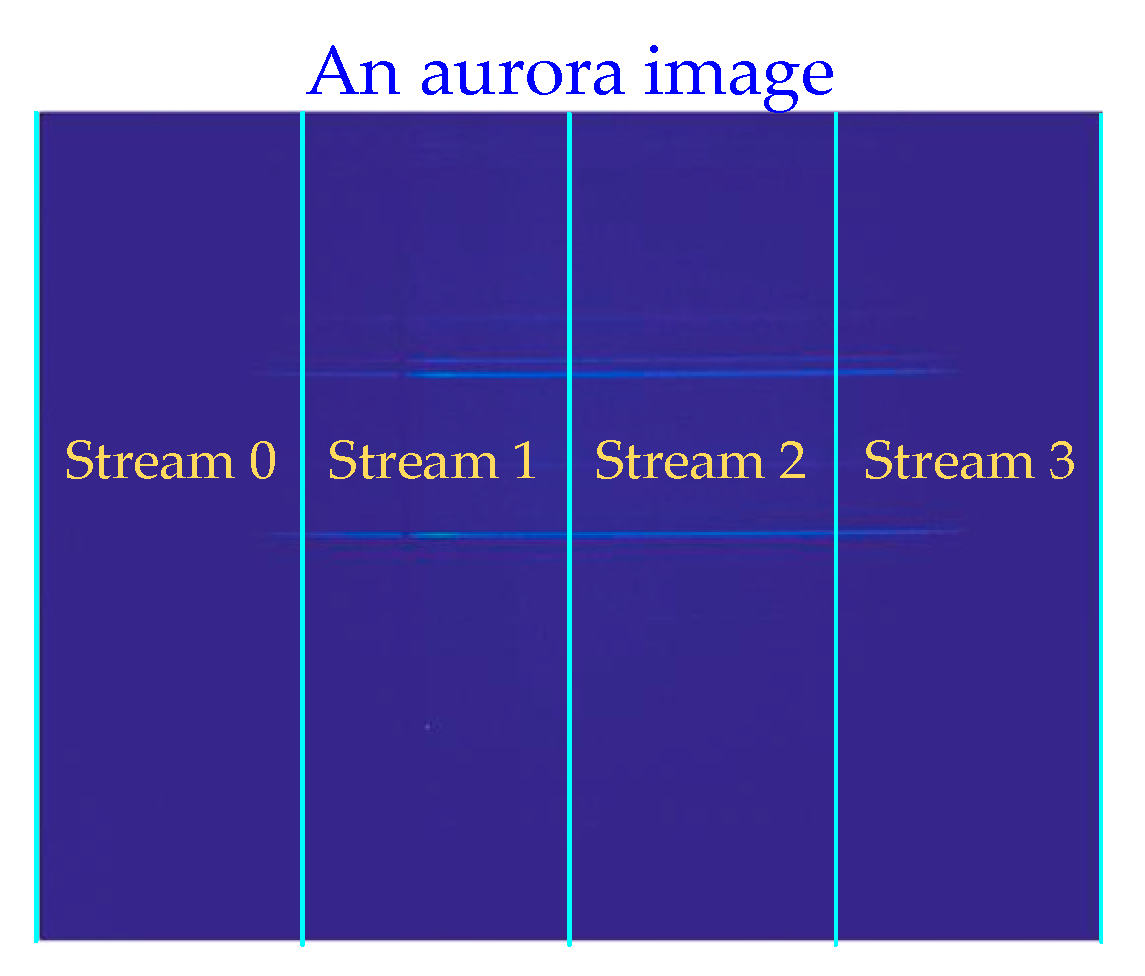
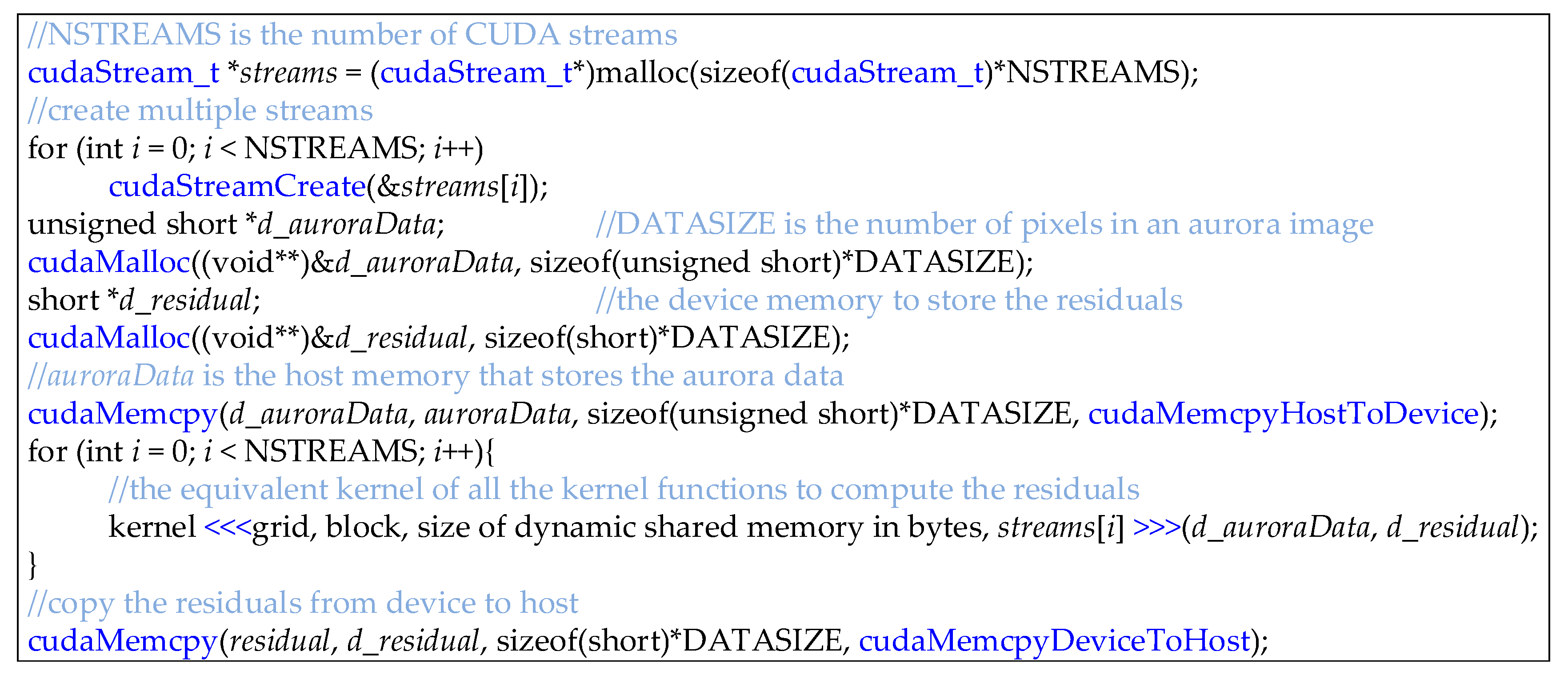
For the optimization of the online DPCM algorithm using the multi-stream technique, the purpose of our scheme is to evenly divide an aurora image by columns and assign each part to a stream, which is because the prediction of a pixel in an aurora image involves all the rows in front of it, as shown in Figure 5. The method for dividing an aurora image into 4 streams is shown in Figure 19, and if there are 2 streams, the division method is similar. Figure 20 shows the CUDA codes of the multi-stream technique. All of the CUDA kernels, including the CTCMulKernel, the CTCBlockPrefixKernel, the matrixInverseKernel, and so on, are equivalent to one kernel, whose input is the aurora data and output is the residual. Note that the aurora data is copied to the device using the synchronous function cudaMemcpy(), which will block the host until the data transfer is finished, rather than the asynchronous function cudaMemcpyAsync(), which allows each stream to copy the data assigned to it from host to device asynchronously. This is because the aurora data is stored by rows but assigned to each stream by columns, so each stream cannot copy the aurora data assigned to the device by calling cudaMemcpyAsync() once, unless the aurora data assigned to each stream is prepared in advance on the host, but this requires extra time. The reason for copying the residual using cudaMemcpy() is similar.
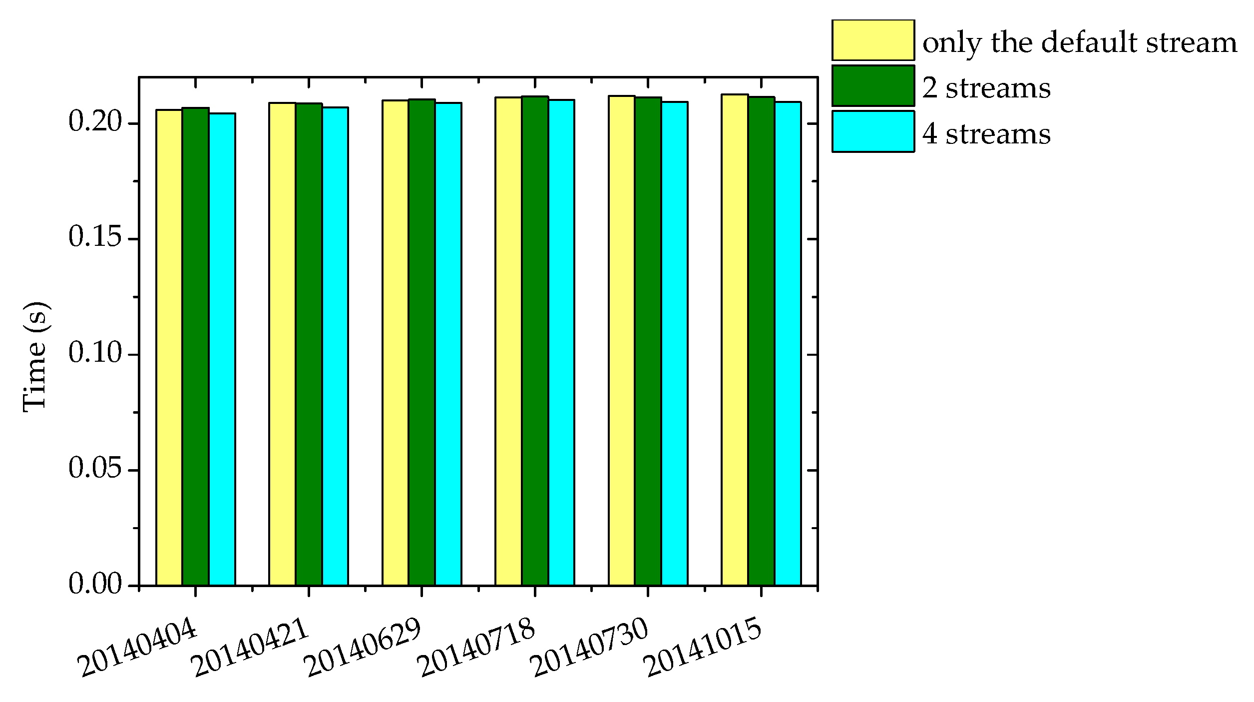
Figure 21 shows the execution time of the parallel implementation of the online DPCM algorithm using two streams and four streams. The time for each day is the average time for 100 aurora spectral images evenly selected from the data of each day. The speed of using the default stream has been shown in Table 1, and here the aim is to make a comparison with the speed using multiple streams. It can be seen that the speed of these three implementations is basically the same, which is because the occupancy of the SM of the three kernels CTCMulKernel, CTCBlockPrefixKernel, and matrixInverseKernel, which accounts for more than 84% of the total time (Table 2), is very high (Table 3), and the occupancy of the SM of other kernels is actually also very high. In a multi-stream program, if a kernel function in one stream has been started, the kernel function in another stream can be started only when there are enough available SMs, otherwise, there will be no overlap of kernel functions, and thus cannot contribute to reducing the total execution time.
4.4. The Parallel Implementation of the Online DPCM Algorithm using Multi-GPU Technique
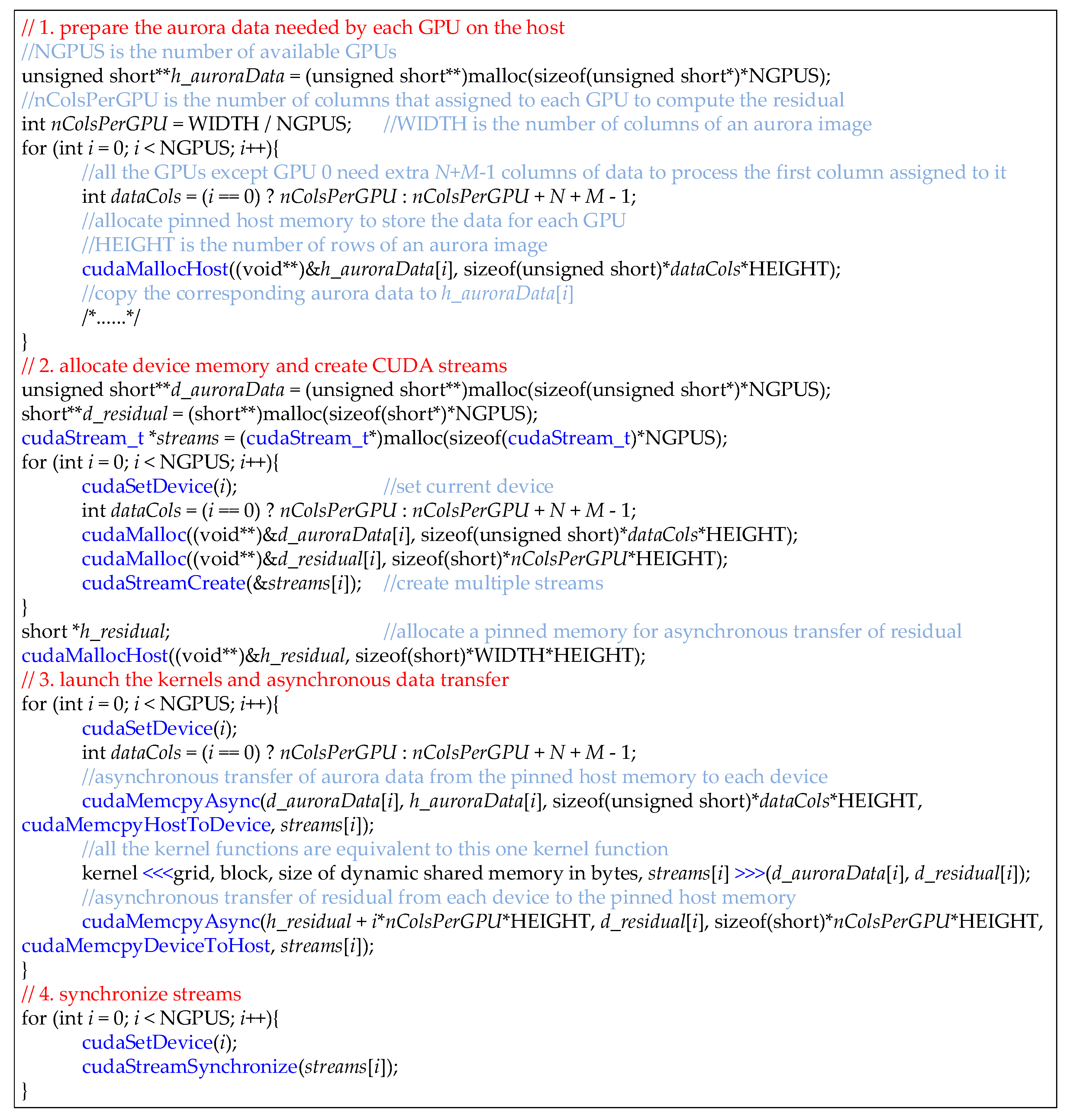
To calculate with multiple GPUs, a programmer needs to subdivide a large calculation problem into several small subproblems and distribute each subproblem to a GPU. All of the GPUs run concurrently, and as a result, the total execution time is reduced. When implementing the online DPCM algorithm using multiple GPUs, the method for subdividing the calculation task is the same as that when using multiple streams, that is, evenly divide the aurora image by columns and distribute each part to a GPU. However, each GPU has its own memory, unlike in multi-stream programming, where all the streams use the same GPU’s memory. Therefore, the aurora data cannot be transmitted to the device by calling the cudaMemcpy() once, as in Figure 20; we must transmit the aurora data assigned to each GPU to the memory of each GPU using the cudaMemcpyAsync(), and the purpose of the preparation before the transmission is to prepare the data for each GPU in advance on the host, though this requires extra time. In addition, the residual computed by each GPU is stored on the memory of each GPU, so we must transfer it to the host using cudaMemcpyAsync() as well, rather than cudaMemcpy(). Some core CUDA codes of the multi-GPU implementation are presented in Figure 22.
The first part in Figure 22 is to prepare the data for each GPU. The nColsPerGPU is the number of columns that are assigned to each GPU. The dataCols is the number of columns that each GPU needs to predict the nColsPerGPU columns of pixels, and this is nColsPerGPU + N + M − 1, except for GPU 0. This is because each pixel requires N + M − 1 previous columns to predict it, as shown in Figure 5, but there is no data before the data assigned to GPU 0, and the initial several columns of data of GPU 0 are predicted using the actual available data. The cudaMallocHost() is a CUDA function to allocate pinned host memory, and the reason for allocating pinned host memory for h_auroraData[i] is that cudaMemcpyAsync() requires the host memory to be pinned memory. The second part is to allocate device memory to store the aurora data and residual for each GPU, and create a stream for each GPU. In the third part, first, the aurora data required by each GPU is asynchronously transmitted from the pinned host memory h_auroraData[i] to each device. Then, the kernel function is launched to calculate the residual, which is actually the equivalent of all the kernels, including the CTCMulKernel, the CTCBlockPrefixKernel, the matrixInverseKernel, and so on. Finally, the residual is copied asynchronously from each device to the pinned host memory h_residual.
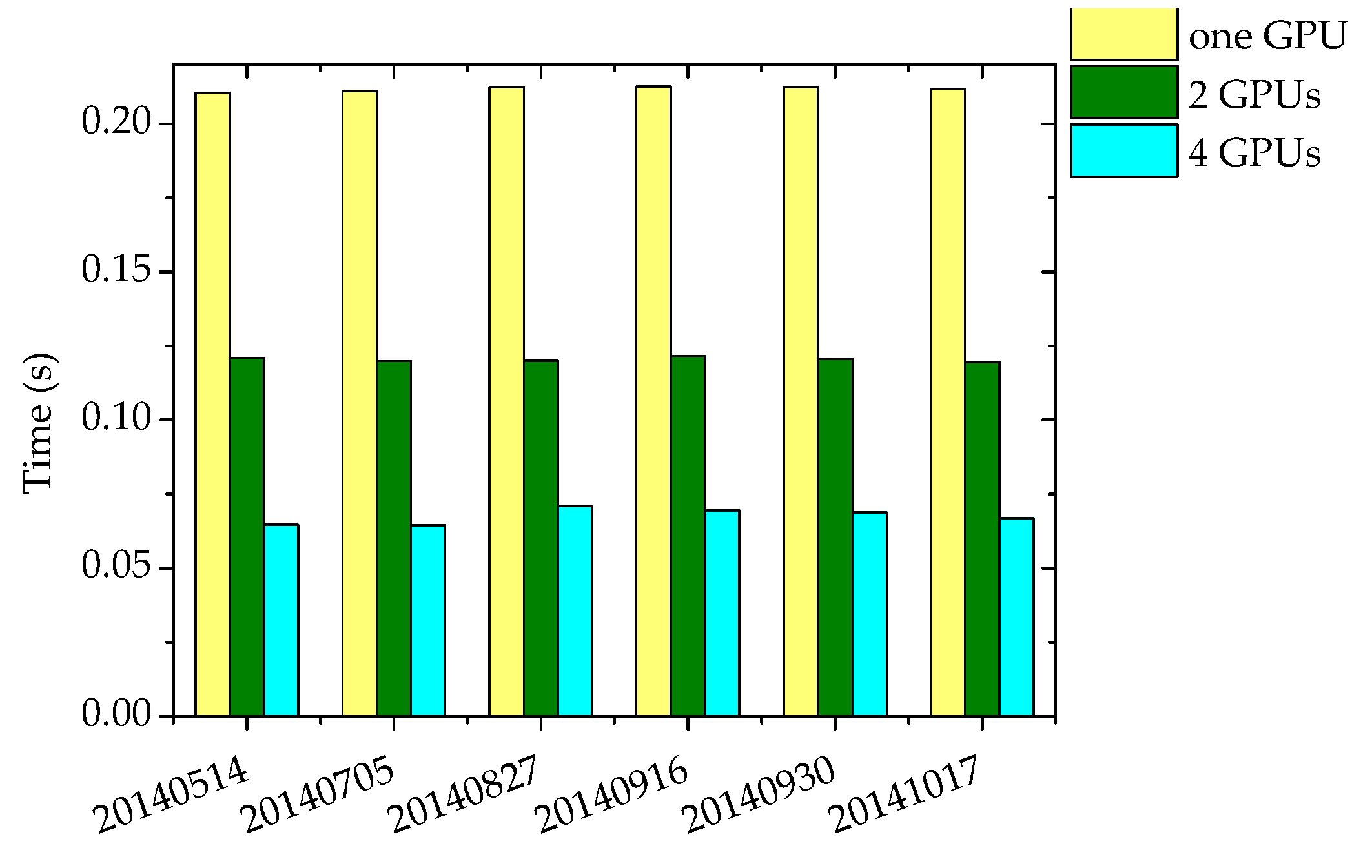
The speed of the multi-GPU implementation using 2 GPUs and 4 GPUs is shown in Table 4. The time for each day is the average time for 100 aurora spectral images evenly selected from the data of each day. It can be seen that the execution time is about 0.12 s when using 2 GPUs, and when the number of GPUs increases to 4, the execution time is between 0.06 s and 0.07 s, which is much less than the 15 s aurora data acquisition time interval. The speedup is the ratio of the serial time to the 2 GPUs time and the 4 GPUs time, respectively.
Furthermore, the speed comparison between using one GPU, 2 GPUs, and 4 GPUs is depicted in Figure 23. The performance of using one GPU has been shown in Section 4.2 and here it is compared with using multiple GPUs. It can be seen that when the number of GPUs is doubled, the time is reduced by about half. This is because when the number of GPUs is doubled, the amount of data processed by each GPU is reduced by half. Note that the time is not exactly cut in half, but always slightly more than a half. This is because as the number of GPUs increases, the overheads increase too, such as the device startup overhead and the kernel launch overhead.
5. Conclusions
This paper introduces the parallel CUDA implementation of the prediction-based online DPCM algorithm for the lossless compression of the aurora spectral data. The first step of the online DPCM method is to compute the prediction coefficients using the least square method, then use the prediction coefficients to compute the predicted value of each pixel, subtract the predicted value from the original value to get the residual, and finally, encode the residual. In order to improve the compression performance of the online DPCM algorithm, we proposed two improvements. The first is to build multiple equations using each of the rows before the current pixel when computing the prediction coefficients, and the other is to apply a dual-threshold method to the encoding of the residual. In the CUDA implementation of the online DPCM, we focus on the multiplication of matrices CT and C and the inversion of the matrix CTC. A decomposition method, which decompose the multiplication of CT and C into the addition of many small matrices, is proposed to remove redundant data access and calculations. In addition, the multi-stream technique and the multi-GPU technique are used to optimize the CUDA implementation. Finally, the average compression time for an aurora spectral image is about 0.06 s when using 4 GPUs.
Since aurorae have the characteristic of instantaneous change and are captured continuously, several consecutive aurora spectral images in time direction should have some correlation. Therefore, in the future work, we plan to apply 3-D methods to aurora spectral image compression to utilize the correlations in time direction, which is impossible for 2-D methods. Although the 3-D methods are more likely to cause transmission errors than 2-D methods, as illustrated in Section 1, we can decorrelate these by grouping only a few aurora spectral images, such as 3–6 frames, to minimize transmission errors. We believe that the improved compression gains justify the increased transmission errors.
Author Contributions
Conceptualization, J.W. and J.L.; Methodology, J.L.; Software, J.L.; Validation, J.L., J.W. and G.J.; Formal Analysis, J.L.; Investigation, J.L.; Resources, J.W.; Data Curation, J.W.; Writing-Original Draft Preparation, J.L.; Writing-Review & Editing, J.W.; Visualization, G.J.; Supervision, J.W.; Project Administration, J.W.; Funding Acquisition, J.W.
Funding
This research was funded by National Natural Science Foundation of China, numbers 61775175 and 61771378.
Acknowledgments
We thank all the editors and reviewers for their valuable comments that greatly improved the presentation of this paper. We thank the Polar Research Institute of China for providing the aurora spectral data.
Conflicts of Interest
The authors declare no conflict of interest.
References
- Kong, W.; Wu, J. Fast DPCM scheme for lossless compression of aurora spectral images. In Proceedings of the High-Performance Computing in Geoscience and Remote Sensing VI, Edinburgh, UK, 26 September 2016; p. 100070M. [Google Scholar] [CrossRef]
- Kong, W.; Wu, J.; Hu, Z.; Anisetti, M.; Damiani, E.; Jeon, G. Lossless compression for aurora spectral images using fast online bi-dimensional decorrelation method. Inf. Sci. 2017, 381, 33–45. [Google Scholar] [CrossRef]
- Wells, D.C.; Greisen, E.W.; Harten, R.H. FITS—A flexible image transport system. Astron. Astrophys. Suppl. 1981, 44, 363. [Google Scholar]
- Aiazzi, B.; Alparone, L.; Baronti, S. Near-lossless image compression by relaxation-labelled prediction. Signal Process. 2002, 82, 1619–1631. [Google Scholar] [CrossRef]
- Aiazzi, B.; Alparone, L.; Baronti, S. Fuzzy logic-based matching pursuits for lossless predictive coding of still images. IEEE Trans. Fuzzy Syst. 2002, 10, 473–483. [Google Scholar] [CrossRef]
- Aiazzi, B.; Alparone, L.; Baronti, S. Context modeling for near-lossless image coding. IEEE Signal Process. Lett. 2002, 9, 77–80. [Google Scholar] [CrossRef]
- Mielikainen, J.; Toivanen, P. Clustered dpcm for the lossless compression of hyperspectral images. IEEE Trans. Geosci. Remote Sens. 2003, 41, 2943–2946. [Google Scholar] [CrossRef]
- Martin, G. Range encoding: An algorithm for removing redundancy from a digitised message. In Proceedings of the Video and Data Recording Conference, Southampton, UK, 24–27 July 1979. [Google Scholar]
- Kong, W.; Wu, J. A lossless compression algorithm for aurora spectral data using online regression prediction. In Proceedings of the High-Performance Computing in Remote Sensing V, Toulouse, France, 21 September 2015; p. 964611. [Google Scholar] [CrossRef]
- Weinberger, M.J.; Seroussi, G.; Sapiro, G. LOCO-I: A low complexity, context-based, lossless image compression algorithm. In Proceedings of the Data Compression Conference-DCC 96, Snowbird, UT, USA, 31 March–3 April 1996; pp. 140–149. [Google Scholar] [CrossRef]
- Weinberger, M.J.; Seroussi, G.; Sapiro, G. The LOCO-I lossless image compression algorithm: Principles and standardization into JPEG-LS. IEEE Trans. Image Process. 2000, 9, 1309–1324. [Google Scholar] [CrossRef]
- Taubman, D.S.; Marcellin, M.W. JPEG2000: Standard for interactive imaging. Proc. IEEE 2002, 90, 1336–1357. [Google Scholar] [CrossRef]
- Wu, X.; Memon, N. Context-based, adaptive, lossless image coding. IEEE Trans. Commun. 1997, 45, 437–444. [Google Scholar] [CrossRef]
- Kim, B.J.; Pearlman, W.A. An Embedded Wavelet Video Coder Using Three-Dimensional Set Partitioning in Hierarchical Trees (SPIHT). In Proceedings of the Conference on Data Compression, Snowbird, UT, USA, 25–27 March 1997; p. 251. [Google Scholar] [CrossRef]
- Lucas, L.F.R.; Rodrigues, N.M.M.; Cruz, L.A.d.S.; Faria, S.M.M.d. Lossless Compression of Medical Images Using 3-D Predictors. IEEE Trans. Med Imaging 2017, 36, 2250–2260. [Google Scholar] [CrossRef]
- Xiaolin, W.; Memon, N. Context-based lossless interband compression-extending CALIC. IEEE Trans. Image Process. 2000, 9, 994–1001. [Google Scholar] [CrossRef] [Green Version]
- Tang, X.; Pearlman, W.A. Three-dimensional wavelet-based compression of hyperspectral images. In Hyperspectral Data Compression; Springer: Boston, MA, USA, 2006; pp. 273–308. [Google Scholar] [CrossRef]
- Zhang, J.; Fowler, J.E.; Liu, G. Lossy-to-Lossless Compression of Hyperspectral Imagery Using Three-Dimensional TCE and an Integer KLT. IEEE Geosci. Remote Sens. Lett. 2008, 5, 814–818. [Google Scholar] [CrossRef] [Green Version]
- Karami, A.; Beheshti, S.; Yazdi, M. Hyperspectral image compression using 3D discrete cosine transform and support vector machine learning. In Proceedings of the 2012 11th International Conference on Information Science, Signal Processing and their Applications (ISSPA), Montreal, QC, Canada, 2–5 July 2012; pp. 809–812. [Google Scholar] [CrossRef]
- Aiazzi, B.; Alparone, L.; Baronti, S.; Lastri, C. Crisp and Fuzzy Adaptive Spectral Predictions for Lossless and Near-Lossless Compression of Hyperspectral Imagery. IEEE Geosci. Remote Sens. Lett. 2007, 4, 532–536. [Google Scholar] [CrossRef]
- Simek, V.; Asn, R.R. GPU Acceleration of 2D-DWT Image Compression in MATLAB with CUDA. In Proceedings of the 2008 Second UKSIM European Symposium on Computer Modeling and Simulation, Liverpool, UK, 8–10 September 2008; pp. 274–277. [Google Scholar] [CrossRef]
- Tenllado, C.; Setoain, J.; Prieto, M.; Piñuel, L.; Tirado, F. Parallel Implementation of the 2D Discrete Wavelet Transform on Graphics Processing Units: Filter Bank versus Lifting. IEEE Trans. Parallel Distrib. Syst. 2008, 19, 299–310. [Google Scholar] [CrossRef] [Green Version]
- Jozef, Z.; Matus, C.; Michal, H. Graphics processing unit implementation of JPEG2000 for hyperspectral image compression. J. Appl. Remote Sens. 2012, 6, 011507. [Google Scholar] [CrossRef]
- Santos, L.; Magli, E.; Vitulli, R.; López, J.F.; Sarmiento, R. Highly-Parallel GPU Architecture for Lossy Hyperspectral Image Compression. IEEE J. Sel. Top. Appl. Earth Obs. Remote Sens. 2013, 6, 670–681. [Google Scholar] [CrossRef]
- Keymeulen, D.; Aranki, N.; Hopson, B.; Kiely, A.; Klimesh, M.; Benkrid, K. GPU lossless hyperspectral data compression system for space applications. In Proceedings of the 2012 IEEE Aerospace Conference, Big Sky, MT, USA, 3–10 March 2012; pp. 1–9. [Google Scholar] [CrossRef]
- Wu, Z.; Shi, L.; Li, J.; Wang, Q.; Sun, L.; Wei, Z.; Plaza, J.; Plaza, A. GPU Parallel Implementation of Spatially Adaptive Hyperspectral Image Classification. IEEE J. Sel. Top. Appl. Earth Obs. Remote Sens. 2018, 11, 1131–1143. [Google Scholar] [CrossRef]
- CUBLAS_Library. Available online: https://docs.nvidia.com/cuda/cublas/#axzz4h7431Tsi (accessed on 22 May 2019).
- CUDA_C_Programming_Guide. Available online: https://docs.nvidia.com/cuda/cuda-c-programming-guide/#axzz4dQa7XYMd (accessed on 22 May 2019).
- Juanjuan, B.; Ling, G.; Lidong, H. Constructing windows+gcc+mpi+omp and performance testing with Gauss-Jordan elimination method in finding the inverse of a matrix. In Proceedings of the 2010 International Conference On Computer Design and Applications, Qinhuangdao, China, 25–27 June 2010. [Google Scholar] [CrossRef]
- Nyokabi, G.J.; Salleh, M.; Mohamad, I. NTRU inverse polynomial algorithm based on circulant matrices using gauss-jordan elimination. In Proceedings of the 2017 6th ICT International Student Project Conference (ICT-ISPC), Skudai, Malaysia, 23–24 May 2017; pp. 1–5. [Google Scholar] [CrossRef]
- 7-Zip. Available online: https://www.7-zip.org/ (accessed on 22 May 2019).
- Burrows, M.; Wheeler, D.J. A Block-Sorting Lossless Data Compression Algorithm. SRC Res. Rep. 1994. [Google Scholar]
- Shkarin, D. PPM: One step to practicality. In Proceedings of the DCC 2002, Data Compression Conference, Snowbird, UT, USA, 2–4 April 2002; pp. 202–211. [Google Scholar] [CrossRef]
- Cleary, J.; Witten, I. Data Compression Using Adaptive Coding and Partial String Matching. IEEE Trans. Commun. 1984, 32, 396–402. [Google Scholar] [CrossRef]
Figure 1.
Two aurora spectral images captured at the Zhongshan Station. Each aurora spectral image has 1024 spectral bands and 1024 spatial sampling points. The color bar on the right is used to indicate the value of each color.
Figure 1.
Two aurora spectral images captured at the Zhongshan Station. Each aurora spectral image has 1024 spectral bands and 1024 spatial sampling points. The color bar on the right is used to indicate the value of each color.

Figure 2.
A small part of an aurora image that is used for the prediction of a certain pixel xm,n.

Figure 3.
The three areas A1, A2, and A3 cannot be predicted using the least square method.

Figure 4.
An example illustrating how to create multiple equations with a row of an aurora image.

Figure 5.
A1(xm,n) is the area that will be used to compute the prediction coefficients of xm,n when using the original online DPCM (Differential Pulse Code Modulation) method, and A1(xm,n) + A3(xm,n) is the area that will be used when using the improved online DPCM method.
Figure 5.
A1(xm,n) is the area that will be used to compute the prediction coefficients of xm,n when using the original online DPCM (Differential Pulse Code Modulation) method, and A1(xm,n) + A3(xm,n) is the area that will be used when using the improved online DPCM method.

Figure 6.
The upper part is the histogram of the aurora spectral image captured on October 17, 2014, at 17:41:20, and the lower part is the magnified view of the shaded part. It can be seen that the maximum pixel value is near 9000, but most of the pixels are within 500. The large majority of the pixel values do not appear in the shaded part, and the maximum number of occurrences is only 4.

Figure 7.
The upper part is the histogram of the residual image of the aurora spectral image in Figure 6; the lower left part is the magnified view of shade1. We can see that most of the residuals are around 0. The lower right part is the magnified view of shade2, where it can be seen that the largest residual is greater than 30,000, but most of the residual values do not appear in shade2, and the remaining residuals only appear once.

Figure 8.
The variation of the bitrate with the three parameters N, M, and T. The bitrate is the average bitrate of each day, and the five days in each subfigure are randomly selected from the 2014 aurora spectral data set.
Figure 8.
The variation of the bitrate with the three parameters N, M, and T. The bitrate is the average bitrate of each day, and the five days in each subfigure are randomly selected from the 2014 aurora spectral data set.

Figure 9.
An example illustrating the thread structure of a kernel function.

Figure 10.
An example illustrating the decomposition method for the multiplication of matrices CT and C.
Figure 10.
An example illustrating the decomposition method for the multiplication of matrices CT and C.

Figure 11.
The method for computing a series of matrices, CT(x1,n)C(x1,n), CT(x2,n)C(x2,n), …, CT(xm,n)C(xm,n). Ci,n (i = 0, 1, …, m − 1) is the matrix built with row i of an aurora image when predicting the pixels in column n. The symbol “⊕” represents addition.
Figure 11.
The method for computing a series of matrices, CT(x1,n)C(x1,n), CT(x2,n)C(x2,n), …, CT(xm,n)C(xm,n). Ci,n (i = 0, 1, …, m − 1) is the matrix built with row i of an aurora image when predicting the pixels in column n. The symbol “⊕” represents addition.

Figure 12.
The upper part shows an example illustrating the idea of computing the prefix sum of an array in parallel, and the lower part presents the CUDA (Compute Unified Device Architecture) codes. The symbol “⊕” represents addition.
Figure 12.
The upper part shows an example illustrating the idea of computing the prefix sum of an array in parallel, and the lower part presents the CUDA (Compute Unified Device Architecture) codes. The symbol “⊕” represents addition.

Figure 13.
Parallel implementation of prefix summing of an array of the last element of all the warps in a thread block. The prefix sum of each warp has been calculated using the method in Figure 12. Combining Figure 12 with Figure 13, we get the prefix sum of each thread block in a thread grid.

Figure 14.
The thread structure for CTCBlockPrefixKernel.

Figure 15.
The CUDA kernel function for the multiplication of matrices CTi,n and Ci,n.

Figure 16.
The CUDA kernel function for the computation of the inverse matrix of CTC.

Figure 17.
Average bitrate of the online DPCM (Differential Pulse Code Modulation) algorithm and several other lossless compression algorithms on the aurora spectral data of 9 days. The average represents the average bitrate of each algorithm on these 9 days.
Figure 17.
Average bitrate of the online DPCM (Differential Pulse Code Modulation) algorithm and several other lossless compression algorithms on the aurora spectral data of 9 days. The average represents the average bitrate of each algorithm on these 9 days.

Figure 18.
An example timeline of a CUDA application with 4 streams.

Figure 19.
The method for dividing an aurora image to four streams.

Figure 20.
The CUDA codes of the online DPCM algorithm using multi-stream technique.

Figure 21.
The comparison in speed between the parallel implementation of the online DPCM algorithm using two streams, four streams, and the default stream.
Figure 21.
The comparison in speed between the parallel implementation of the online DPCM algorithm using two streams, four streams, and the default stream.

Figure 22.
The core CUDA codes for the multi-GPU implementation of the online DPCM algorithm.

Figure 23.
The comparison in speed between the parallel implementation of the online DPCM algorithm using 2 GPUs, 4 GPUs, and only one GPU.
Figure 23.
The comparison in speed between the parallel implementation of the online DPCM algorithm using 2 GPUs, 4 GPUs, and only one GPU.


Table 1.
The execution time for three different implementations of the online DPCM algorithm. The speedup is the ratio of the serial decomposed time to the parallel time.
Table 1.
The execution time for three different implementations of the online DPCM algorithm. The speedup is the ratio of the serial decomposed time to the parallel time.
| Implementation | Serial Direct Time (s) | Serial Decomposed Time (s) | Parallel Time (s) | Speedup | |
|---|---|---|---|---|---|
| Data | |||||
| 20140328 | 869.16 | 3.75 | 0.19 | 19.7 | |
| 20140404 | 872.56 | 3.74 | 0.21 | 17.8 | |
| 20140425 | 872.28 | 3.74 | 0.21 | 17.8 | |
| 20140629 | 872.24 | 3.74 | 0.21 | 17.8 | |
| 20140705 | 872.12 | 3.74 | 0.21 | 17.8 | |
| 20140718 | 869.67 | 3.74 | 0.21 | 17.8 | |
| 20140730 | 870.48 | 3.73 | 0.21 | 17.8 | |
| 20140827 | 872.68 | 3.74 | 0.21 | 17.8 | |
Table 2.
The time and ratio of three CUDA kernel functions and two data transfers on two aurora images 20140514_133241 and 20140923_155500.
Table 2.
The time and ratio of three CUDA kernel functions and two data transfers on two aurora images 20140514_133241 and 20140923_155500.
| 20140514_133241 | 20140923_155500 | |||
|---|---|---|---|---|
| Time | Ratio (%) | Time | Ratio (%) | |
| CTCMulKernel | 10.820 ms | 5.71 | 10.759 ms | 5.71 |
| CTCBlockPrefixKernel | 11.920 ms | 6.29 | 11.857 ms | 6.29 |
| matrixInverseKernel | 137.29 ms | 72.41 | 136.42 ms | 72.36 |
| memcpyHtoD | 191.24 us | 0.10 | 194.25 us | 0.10 |
| memcpyDtoH | 161.32 us | 0.09 | 161.32 us | 0.09 |
Table 3.
The achieved_occupancy and gld_throughput of the three kernel functions on two aurora images 20140514_133241 and 20140923_155500.
Table 3.
The achieved_occupancy and gld_throughput of the three kernel functions on two aurora images 20140514_133241 and 20140923_155500.
| 20140514_133241 | 20140923_155500 | |||
|---|---|---|---|---|
| achieved_occupancy | gld_throughput | achieved_occupancy | gld_throughput | |
| CTCMulKernel | 87.06% | 5.43 GB/s | 87.24% | 4.61 GB/s |
| CTCBlockPrefixKernel | 94.88% | 321.91 GB/s | 94.88% | 310.63 GB/s |
| matrixInverseKernel | 99.63% | 183.53 GB/s | 99.63% | 183.21 GB/s |
Table 4.
The execution time for the serial and two multi-GPU (Graphics Processing Unit) implementations of the online DPCM algorithm.
Table 4.
The execution time for the serial and two multi-GPU (Graphics Processing Unit) implementations of the online DPCM algorithm.
| 20140514 | 20140705 | 20140827 | 20140916 | 20140930 | 20141017 | ||
|---|---|---|---|---|---|---|---|
| Serial time(s) | 3.74 | 3.74 | 3.74 | 3.74 | 3.74 | 3.74 | |
| 2 GPUs | Time(s) | 0.12 | 0.12 | 0.12 | 0.12 | 0.12 | 0.12 |
| Speedup | 31.2 | 31.2 | 31.2 | 31.2 | 31.2 | 31.2 | |
| 4 GPUs | Time(s) | 0.06 | 0.06 | 0.07 | 0.07 | 0.07 | 0.07 |
| Speedup | 62.3 | 62.3 | 53.4 | 53.4 | 53.4 | 53.4 | |
© 2019 by the authors. Licensee MDPI, Basel, Switzerland. This article is an open access article distributed under the terms and conditions of the Creative Commons Attribution (CC BY) license (http://creativecommons.org/licenses/by/4.0/).
Share and Cite
MDPI and ACS Style
Li, J.; Wu, J.; Jeon, G. GPU-Based Lossless Compression of Aurora Spectral Data using Online DPCM. Remote Sens. 2019, 11, 1635. https://doi.org/10.3390/rs11141635
AMA Style
Li J, Wu J, Jeon G. GPU-Based Lossless Compression of Aurora Spectral Data using Online DPCM. Remote Sensing. 2019; 11(14):1635. https://doi.org/10.3390/rs11141635
Chicago/Turabian StyleLi, Jiaojiao, Jiaji Wu, and Gwanggil Jeon. 2019. "GPU-Based Lossless Compression of Aurora Spectral Data using Online DPCM" Remote Sensing 11, no. 14: 1635. https://doi.org/10.3390/rs11141635
Note that from the first issue of 2016, this journal uses article numbers instead of page numbers. See further details here.