Noise Removal from Remote Sensed Images by NonLocal Means with OpenCL Algorithm

Abstract

We introduce a multi-platform portable implementation of the NonLocal Means methodology aimed at noise removal from remotely sensed images. It is particularly suited for hyperspectral sensors for which real-time applications are not possible with only CPU based algorithms. In the last decades computational devices have usually been a compound of cross-vendor sets of specifications (heterogeneous system architecture) that bring together integrated central processing (CPUs) and graphics processor (GPUs) units. However, the lack of standardization resulted in most implementations being too specific to a given architecture, eliminating (or making extremely difficult) code re-usability across different platforms. In order to address this issue, we implement a multi option NonLocal Means algorithm developed using the Open Computing Language (OpenCL) applied to Hyperion hyperspectral images. Experimental results demonstrate the dramatic speed-up reached by the algorithm on GPU with respect to conventional serial algorithms on CPU and portability across different platforms. This makes accurate real time denoising of hyperspectral images feasible.

1. Introduction

Technology for sensors onboard satellites and aircraft is undergoing a fast evolution in terms of better spatial, spectral and time resolution. As a consequence the amount of gathered data dramatically increases. This calls for unprecedented challenges in terms of data transmission, storing and processing. In this respect we mention among imagers the hyperspectral ones (with a number of channels over 200), like AVIRIS [1], Hyperion [2] and PRISMA [3]. A noteworthy category is given by high spectral resolution sounder interferometers (e.g., IASI [4] with its 8K spectral channels). The advent of new concept imaging interferometers onboard geostationary platforms (expected with ongoing METEOSAT Third Generation [5]) boosts the amount of data because of the combination of full hemisphere coverage (8M pixels), hyperspectrality (2K channels) and the low repetition time (60 min). All these concepts are the perfect ground for the big data paradigm, with its challenges in terms of storing, computing and modeling capabilities. In many remote sensing applications methodologies are well consolidated and storing capabilities are sufficient; however computational speed is a critical issue when computational cost scales more than linearly with the size of data and real-time processing is necessary. In this respect Graphical Processing Units (GPUs) are an important part of the rapid development of the general computing architecture and they have received much attention as a hardware platform that is complementary to Central Processing Units (CPU) in modern computers; they became a key technology for big data science for the abatement of computational time and also for boosting Artificial Intelligence (IA) applications. GPUs have small volume and moderate price, providing floating point calculations and highly intensive computation capacity. Signal and image processing for remotely sensed data are an active area of research encompassing dimensionality reduction [6,7,8,9], features extraction [10,11] and compression [12], all tools that are now a firm part of big data science.

Therefore it is easily understandable that during the past few years GPUs have been fast introduced in the remote sensing community for those algorithms that show an inherent parallelization suitable for the architecture. For a general use of GPUs in remote sensing we defer to [13,14,15], which, besides showing general GPU programming designs for remote sensing, also compare Multicore and GPU architectures. The most successful application can be considered the spectral unmixing, where, among other things, algorithms have been developed for estimating the Pixel Purity Index [16], endmember identification [17,18], matrix factorization [19] and unmixing [20,21]. Among other remote sensing applications we recall orthorectification [22], image registration [23], NDVI computation [24] and classification [25,26].

Many proprietary standards and tools have been designed that cover a closed set of architectures and make them work in a suited way really close to the architecture features, but still one of the key challenges in parallel computing is development of a broadly accepted programming model truly supported by a large set of architectures. The lack of standardization results in most applications being too specific for a given architecture, making the portability extremely difficult, that means the possibility of reusing code across different platforms. In turn, the need to improve portability has driven the development of an open computing language (OpenCL) [27,28], that has become a free-standard for cross-platform modern multiprocessors.

In the present paper we consider the problem of noise removal, a preliminary step of many algorithms that process remotely sensed images. Numerous methods have been specifically developed for the remote sensing community, both for optical and active sensors, exploiting the GPU architecture. They are generally sorted according to whether they work in physical space [29,30], in a transformed space [31,32,33] or use variational methods [34,35].

A powerful method among the image processing community for denoising images is NonLocal Means (NLM) [36]. This can be considered a filtering algorithm; however differently from conventional spatial filters, it searches for the closest pixels in the signal domain rather than in the spatial one. In addition the closeness criterion is sought in a region instead of single pixels. Therefore the method is claimed to effectively keep the integrity of the image while removing its noise. The improvement of denoising has a counterpart in that NLM is not local anymore but for each pixel it spans the full image in the search of regions showing similar textures. This makes NLM computational cost in principle quadratic with respect to the number of pixels in an image and therefore highly demanding in terms of computational time. Nevertheless some limited approximated implementations for remote sensing exist exploiting traditional CPU architectures, especially in the SAR community (e.g., [37,38,39]). However they are not suited for real-time applications and are very time consuming even for the preliminary step of bandwidth selection.

Since the pioneering work by NVIDIA [40], variants of the algorithm have been proposed (e.g., [41]). Application to Magnetic Resonance Imaging (MRI) has been developed during recent years [42,43]. The MRI framework naturally adapts to the original NVIDIA work because the T1, T2, PD images acquired there well resemble the RGB images dealt with in [40]. Application of GPU algorithms for NLM to Remote Sensing is limited to Interferometrics Phase Denoising [44]. This is surprising if one considers that the size of the images involved in Remote Sensing is quickly increasing (e.g., very high spatial resolution sensors, increased temporal frequency, high spectral resolution). In particular a high number of spectral bands (up to thousands with respect to the three RGB considered initially by NVIDIA and T1, T2, PD in MRI applications) possibly calls for new and portable algorithms able to better implement this framework even for embedded devices with no available GPUs. In addition the algorithm from NVIDIA of course was explicitly developed for their CUDA programming model, and all applications known in the literature followed the same trend.

Therefore the aim of the paper is to develop a GPU based algorithm for denoising remotely sensed images by NLM at a very high speed, and to estimate its speed-up with respect to traditional architectures on images coming from optical sensors. In addition we intend to develop a multi-platform implementation of NLM able to be run on most computing equipments, including GPU of different architectures and also multi-core CPU.

2. Nonlocal Means for Image Denoising

NonLocal Means (NLM) filter [36] tries to take advantage of the high degree of redundancy of any natural image and it is nowadays considered the state-of-art algorithm for denoising images. It belongs to the class of filtering methodologies but uses a weight function that takes into account the intensity values not only of pixels, but also of their neighborhoods.

Let $\Omega$ be a noisy image of size $(N_x,N_y)$ pixels, with $N=N_x{N}_y$ being the total number of pixels, and let $x_i$ be a corresponding pixel, $x_i\in \Omega$. We denote by $u_i$ and ${\overline{u}}_i$ the original and denoised intensity at pixel $x_i$, respectively. In the formulation [36] of the NLM filter the restored intensity at a generic pixel $x_i$ is computed as a weighted average (also called kernel convolution) of all the pixels $x_j$ in the image belonging to a search volume $V_i\subseteq \Omega$, centered at the pixel $x_i$:

$${\tilde{u}}_i=\sum _{x_j\in V_i}w(x_i,x_j)u_j,$$

(1)

where $w(x_i,x_j)$ is the weight assigned to $u_j$ in removing noise from pixel $x_i$. To be more specific, the weight is an estimate of the similarity between the intensities of two neighborhoods $D_i\subseteq \Omega$ and $D_j\subseteq \Omega$ centered at pixels $x_i$ and $x_j$, respectively, such that

$$w(x_i,x_j)\in [0,1],\sum _{x_j\in V_i}w(x_i,x_j)=1.$$

The definition of the classical NLM filter does not make any assumption about the search volume, it only requires that each pixel can be linked to the others. However for computational reasons it is usually assumed that both neighbors $V_i$ and $D_i$ are taken as boxes of size $(2v_x+1)(2v_y+1)$ and $(2d_x+1)(2d_y+1)$, with $v=(v_x,v_y)$ and $d=(d_x,d_y)$ being the window radii of $V_i$ and $D_i$, respectively, along each spatial direction x, y.

Efros and Leung [45] showed that the $L^2$ distance is a reliable measure for estimating the similarity of image windows in a texture patch. Therefore it can be estimated as the (possibly Gaussian weighted) Euclidean distance ${∥u\left(D_i\right)-u\left(D_j\right)∥}_2^2$ between the patches $u\left(D_i\right)$ and $u\left(D_j\right)$. The weights associated to the quadratic distance introduced in [36] are

$$w(x_i,x_j)=\frac{1}{Z_i}exp\left(-\frac{{∥u\left(D_i\right)-u\left(D_j\right)∥}_2^2}{h^2}\right),$$

where $Z_i$ is a normalization constant to ensure that ${\sum }_{x_j\in V_i}w(x_i,x_j)=1$ and h is a filtering parameter that controls the decay of the exponential function.

Indeed, for each pixel in the image, the distances between the intensity neighborhoods $u\left(D_i\right)$ and $u\left(D_j\right)$ are computed for all pixels $x_j$ contained in $V_i$. The complexity of the filter is of the order of $\mathcal{O}\left(N(2v_x+1)(2v_y+1)(2d_x+1)(2d_y+1)\right)$. The NLM algorithm is proved by [36] to be consistent for every nonnegative h, even if it is usually chosen of order of the standard deviation of the noise, which means to assume that patches can be considered alike if they differ in such quantity. That notwithstanding, the assumption of uniform variance over the image leads to sub-optimal results wherever nonstationary noise is present, so Manjón et al. [46] proposed a local adaptive estimate at the pixel k:

$${\left({\sigma }_k\right)}^2=\underset{S_k}{min}\left(d(R\left(S_k\right),R\left(S_l\right))\right),k\ne l,R\left(S_l\right)=u_l-\varrho \left(u_l\right),$$

(2)

$S_l$ being the patch centered at the pixel l and $\varrho \left(u_l\right)$ the low-pass filtered intensity estimated as its average in the patch $S_l$ centered on pixel l. Based on experimental arguments we use:

$${\left(\widetilde{{\sigma }_i}\right)}^2=\delta {\left({\sigma }_i\right)}^2,with\delta \in (0,1].$$

(3)

This allows one to regulate the reduction of the overestimation of noise variance occurring in similar patches.

2.1. Multi-Platform NLM OpenCL Implementation

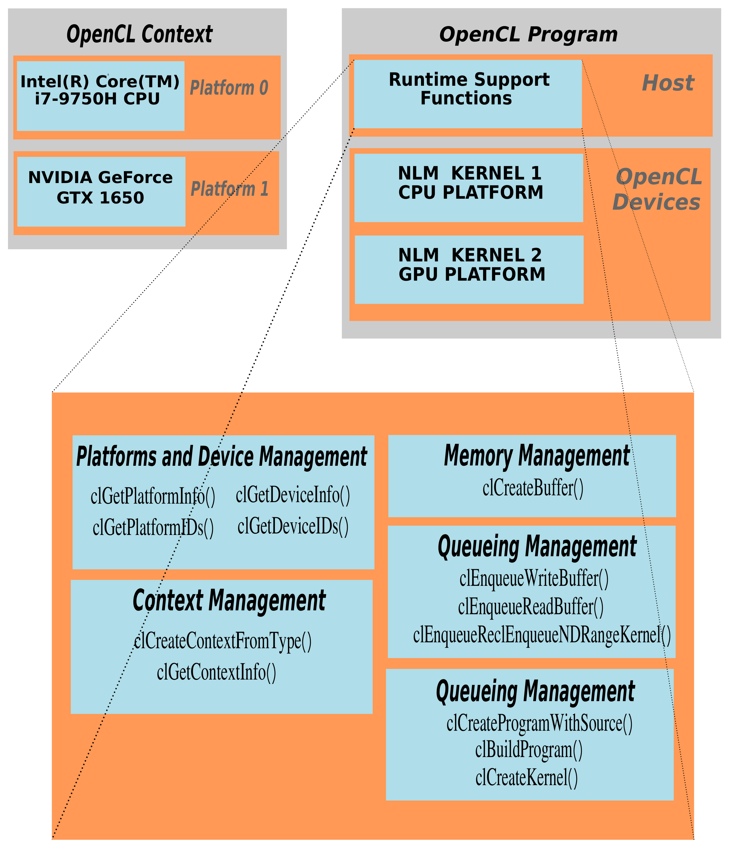
We have developed multi-platform NLM algorithms using an OpenCL C language, a restricted version of the $C99$ language with extensions appropriate for executing data-parallel code. The level of complexity imposed by OpenCL is similar to other dedicated programming models such as Compute Unified Device Architecture (CUDA) developed by NVIDIA. OpenCL defines an application programming interface (API) for cross-platform modern multiprocessors by a group of manufacturers such as Apple, Intel, AMD, or NVIDIA itself. OpenCL is managed by the no-profit technology consortium KhronosGroup (Apple, IBM, NVIDIA, AMD, Intel, ARM, etc.).

In OpenCL, a system consists of a host (the CPU), and one or more devices, which are massively parallel processors, allowing one to define a kernel or group of kernels that exploit multi-thread-based parallelism and are loaded and executed on a multicore platform.

A kernel is a function which contains a block of instructions that are executed by the work-thread group. The kernels exhibit the important property of data parallelism, allowing arithmetic operations to be simultaneously performed on different parts of the data by means of several work-items. A group of work-items forms a work group that runs on a single compute unit. The maximum dimension of each work-group depends on the specifications of the device in use, usually up to 1024 work-items in GPUs.

In practice, work-items (threads) are gathered in work-groups (threads blocks).

A work-item is distinguished from other executed work-items within the collection by its global ID and local ID. Each work-item is identified by its global ID $(g_x,g_y)$ or by the combination of the work-group ID $(w_x,w_y)$, the size of each work-group $(S_x,S_y)$, and the local ID $(s_x,s_y)$ inside the work-group.

The memory hierarchy of GPUs is different from that of CPUs. In practice, there are private memory, local memory, constant memory, and global memory. Global memory is the largest memory, but with high latency; it is typically used to store input and output data structures. Constant memory is a small read-only memory, supporting low latency and high bandwidth access when all threads simultaneously access the same location. Local memory can be allocated to a work-group and accessed at a very high speed in a highly parallel manner. Private memory is the region of memory private to a work-item.

As all threads in a work-group can read and write their own local memory, it is a very efficient way for threads to share their input data, and intermediate results can be synchronized via barriers and memory fences.

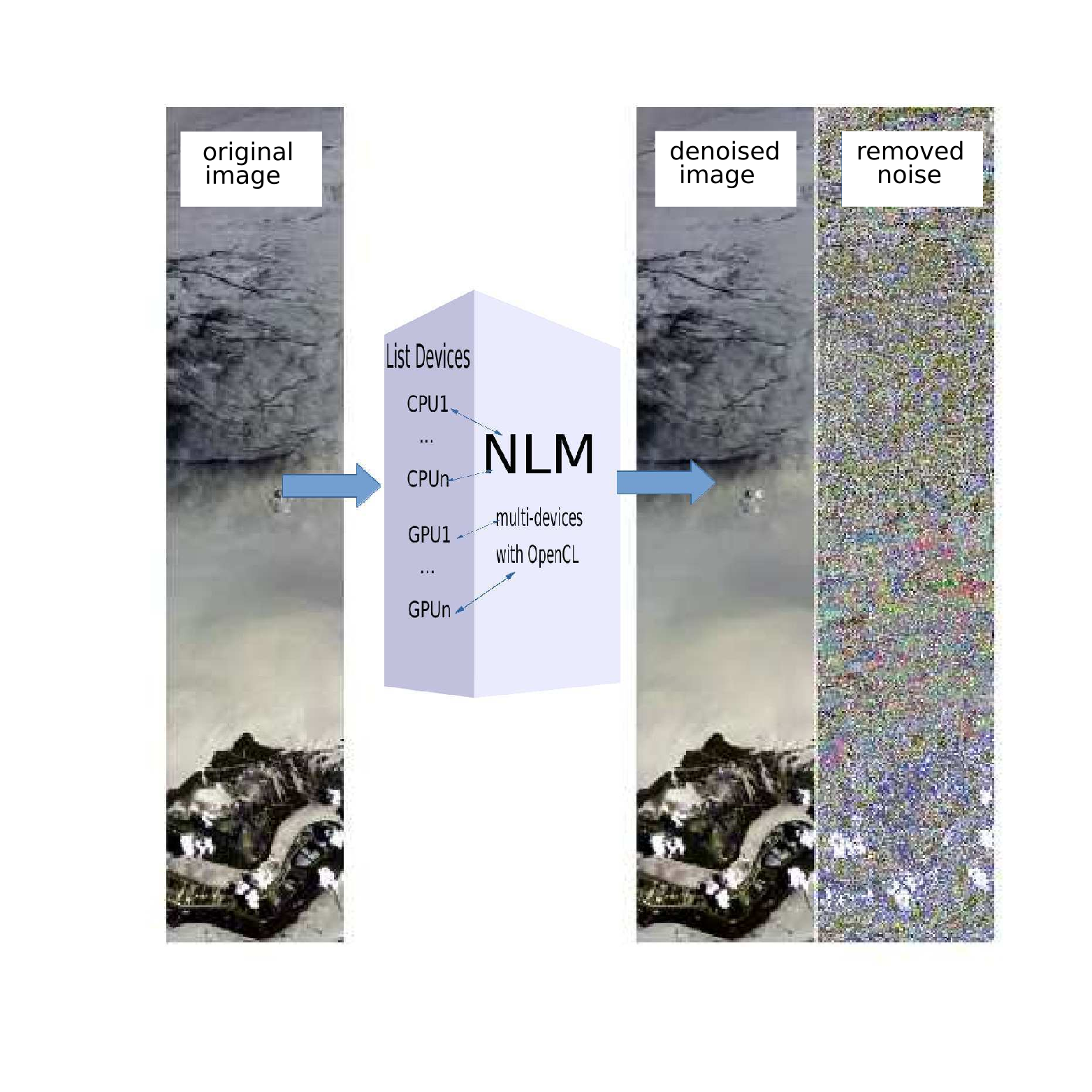
In the initial section of the program, the system is queried, defining the appropriate operating context, specifically the characteristics of the available OpenCL devices, such as the amount of processing units and threads available for computation. Discovering the computational devices available we create two different lists of available devices: One for the CPU device type and the other one for GPU device type, allowing one to choose which kind of device to prefer. If no GPU type device is available, then a CPU device is automatically chosen. Consequently, the OpenCL task scheduler can conveniently split the workload and perform a balanced computation across the system’s resources.

Each block image is processed by a corresponding thread block that executes the NLM filter on a portion of the image and writes back the restored values to the output structure from the device memory to the CPU structure.

Furthermore some support structures are defined as device and host buffers and I/O parameters to regulate the algorithm call. These can be listed as follows:

$\Omega$: Device buffers to load the data;

$\tilde{\Omega }$: Host buffers containing the restored data.

${\sigma }^2$: Host/device buffer containing the estimate noise variance.

$use\_adp\_\sigma$: boolean host/device variable: If this is true then the adaptive noise variance is performed according to (2)–(3).

$\delta$: Host/device buffer with the noise variance regulation measure whenever $use\_adp\_\sigma$ is true (we recall that we use (3)).

d: Similarity radius, constant device buffer.

v: Window radius, constant device buffer.

$N_x$ and $N_y$: Constant device buffers representing the image dimension, width and height, respectively.

$use\_CPU$: Host/device boolean value determining which kind of platform is preferred to operate the computation. If no GPU platform is available then CPU platform is automatically chosen.   

Algorithm 1 describes the classical sequential operations of NLM, whereas Algorithm 2 presents our portable OpenCl implementation.

Algorithm 1NLM_SEQUENTIAL($\Omega$, $\tilde{\Omega }$, ${\sigma }^2$, $use\_adp\_\sigma =\mathrm{false}$, $\delta$, $N_x$, $N_y$, d, v)

$\mathit{patch}\_\mathit{area}=\left(\right(2\ast d+1)\ast (2\ast d+1\left)\right)$ for all$x\in N\_x$do  for all $y\in N\_y$ do   $sum\_w_{x,y}=0$   $cl{r}_{x,y}=0$   for j from $-v$ to $+v$ do    for i from $-v$ to $+v$ do     $w_{i,j}=0$     for m from $-d$ to d do      for n from $-d$ to d do       $w_{i,j}+=d({\Omega }_{x+j+m,y+i+n},{\Omega }_{x+m,y+n})$      end for     end for     $w_{i,j}=exp\left(-\left(w_{i,j}/h^2/patch\_area\right)\right)$     $cl{r}_{x,y}+={\Omega }_{j,i}\ast w_{i,j}$     $sum\_w_{x,y}+=w_{i,j}$    end for   end for   $sum\_w_{x,y}=1/sum\_w_{x,y}$   $cl{r}_{x,y}\ast =sum\_w_{x,y}$   ${\tilde{\Omega }}_{x,y}=cl{r}_{x,y}$  end for end for

Algorithm 2 NLM_OPENCL($\Omega$, $\tilde{\Omega }$, ${\sigma }^2$, $use\_adp\_\sigma =\mathrm{false}$, $\delta$, $N_x$, $N_y$, d, v, $use\_CPU$)

$\mathit{G}\_\mathit{GPU}\leftarrow \varnothing$// list GPU platforms available $\mathit{G}\_\mathit{CPU}\leftarrow \varnothing$// list CPU platforms available // Initialization step: $\mathit{numPlatforms}\leftarrow \mathbf{clGetPlatformIDs}$// recover the number of platforms $\mathit{G}\_\mathit{GPU}\leftarrow \mathbf{clGetDeviceIDs}(\dots ,\mathit{CL}\_\mathit{DEVICE}\_\mathit{TYPE}\_\mathit{GPU},\dots )$// number of available GPUs on the system $\mathit{G}\_\mathit{CPU}\leftarrow \mathbf{clGetDeviceIDs}(\dots ,CL\_DEVICE\_TYPE\_CPU,\dots )$// number of available CPUs on the system if$\mathit{G}\_\mathit{GPU}=\varnothing \mathit{OR}\mathit{use}\_\mathit{CPU}$then $\mathit{\hspace{1em}device}\leftarrow \mathit{FIRST}(\mathit{G}\_\mathit{CPU})$ else $\mathit{\hspace{1em}device}\leftarrow \mathit{FIRST}(\mathit{G}\_\mathit{GPU})$ end if // Computation of the NLM filtered signal step: $\mathbf{cl}\_\mathbf{context}\leftarrow \mathbf{clCreateContext}(\dots ,\mathbf{device},\dots )$// used by the OpenCL runtime for // managing objects such as command-queues, memory, program and kernel objects $\mathbf{cl}\_\mathbf{command}\_\mathbf{queue}\leftarrow \mathbf{clCreateCommandQueue}(\mathit{cl}\_\mathit{context},\mathit{device},\dots )$// creates a command queue associate with the context $\mathbf{cl}\_\mathbf{program}\leftarrow \mathbf{clCreateProgramWithSource}(\mathit{cl}\_\mathit{context},\dots ,\mathit{kernel}\_\mathit{source}\_\mathit{code},\dots )$// creates a program object for a context, and loads the source code specified values $\{\dots ,d,v,N\_x,N\_y\}$ to store into constant memory if$\mathbf{clBuildProgram}(\mathit{cl}\_\mathit{program},\dots ,\mathit{device},\{\dots ,d,v,N\_x,N\_y\},\dots )=\mathit{CL}\_\mathit{SUCCESS}$then  // compiles and links a program executable from the program source cl_program passing the constant parameters $\mathbf{cl}\_\mathbf{mem}\leftarrow \mathbf{clCreateBuffer}(\mathit{context},\{\mathit{CL}\_\mathit{MEM}\_\mathit{READ}\_\mathit{ONLY}|\mathit{CL}\_\mathit{MEM}\_\mathit{USE}\_\mathit{HOST}\_\mathit{PTR}\},|\Omega |,\Omega ,\dots )$ // creates a kernel read only buffer object and referenced by host ptr thanks to {CL_MEM_READ_ONLY|CL_MEM_USE_HOST_PTR} flags  $\mathbf{cl}\_\mathbf{kernel}\leftarrow \mathbf{clCreateKernel}(\mathit{cl}\_\mathit{program},\mathit{kernel}\_\mathit{name},\dots )$// according to $\mathit{use}\_\mathit{adp}\_\sigma$ creates a kernel object with a specific name based on the cl_program to call  // recover information about the thread work group  $\mathit{wg}\_\mathit{multiple}\leftarrow \mathbf{clGetKernelWorkGroupInfo}(\mathit{cl}\_\mathit{kernel},\mathit{device},$  C_KERNEL_PREFERRED_WORK_GROUP_SIZE_MULTIPLE, $\dots )$  According to wg_multiple determines work-group size and number of work-groups all over the data  // set the value to kernel arguments  $\mathbf{clSetKernelArg}(\mathit{kernel},\dots ,|\Omega |,\Omega )$  $\mathbf{clSetKernelArg}(\mathit{kernel},\dots ,|\tilde{\Omega }|,\tilde{\Omega })$  $\mathbf{clSetKernelArg}(\mathit{kernel},\dots ,|\delta |,\delta )$  $\mathbf{clEnqueueNDRangeKernel}(\mathit{cl}\_\mathit{commandQueue},\mathit{cl}\_\mathit{kernel},\dots ,$ number of work-groups, work-group size, $\dots )$// execute all the operations into cl_commandQueue into a cl_kernel on a device  Wait until all the kernel operations have been performed  Collect the restored data to $\tilde{\Omega }$. else  return "Build Program Error!" end if

The denoising filter is computed for all the pixels considering the similarity and window search size.

By observing the program flow in Algorithm 2 the OpenCL runtime is defined by a set of functions that can be globally grouped in Query Platform Info, Contexts, Query Devices, and Runtime API as shown in Figure 1.

3. Materials

3.1. Hardware Work Environment

The experiments have been carried out on a heterogeneous system based on an Intel(R) Core(TM) i7-9750H CPU @2.60GHz processor with six cores and 16GB of DDR4 memory. The following two types of OpenCL Platforms have been considered:

• A CPU, Intel(R) Core(TM) i7-9750H CPU @2.60GHz and Platform Version: OpenCL 2.0 with
  • CL_DEVICE_GLOBAL_MEM_SIZE: 15749 MByte,
  • CL_DEVICE_MAX_CONSTANT_BUFFER_SIZE: 64 KByte,
  • CL_DEVICE_LOCAL_MEM_SIZE: 48 KByte
  • CL_KERNEL_PREFERRED_WORK_GROUP_SIZE_MULTIPLE: 128
  • CL_DEVICE_MAX_WORK_ITEM_SIZES: 8192 / 8192 / 8192
  • CL_DEVICE_MAX_WORK_GROUP_SIZE: 8192
• An NVIDIA GeForce GTX 1650 GPU with 1024 CUDA® Cores operating at 1245 MHz and having 4GB of on-board memory, compute capability 7.5, microarchitecture Turing Generation released on February 2019 and Platform Version: OpenCL 1.2
  • CL_DEVICE_GLOBAL_MEM_SIZE: 15749 MByte,
  • CL_DEVICE_MAX_CONSTANT_BUFFER_SIZE: 128 KByte,
  • CL_DEVICE_LOCAL_MEM_SIZE: 32 KByte
  • CL_KERNEL_PREFERRED_WORK_GROUP_SIZE_MULTIPLE: 32
  • CL_DEVICE_MAX_WORK_ITEM_SIZES: 1024 / 1024 / 1024
  • CL_DEVICE_MAX_WORK_GROUP_SIZE: 1024

3.2. Data Sets

We consider images obtained from the Hyperion sensor onboard EO/1 satellites. Hyperion can be considered as a good proxy of sensor PRISMA, having similar spectral coverage, spectral resolution and spatial resolution.

For this study, we have taken into consideration three Hyperion images with different sizes (see

Table 1. Summary of information on the Hyperion datasets used for the analysis: Identity, location, date and size of the images.

Image	Identity	Location	Date	Size (Pixels)
Ajka	EO1H1890272010282110KF_1	Ajka (Hungary)	19 October 2010	$400\times 256$
Oil Spill	EO1H0210402010195110KF_1R	Gulf of Mexico	14 July 2010	$1200\times 256$
Desert	O1H1790412015255110P0_1R	Egypt	15 September 2015	$6981\times 256$

for a summary). As the computational time of the algorithms does not depend on the scene of the image, but only on its size, the images are shown only as a reference.

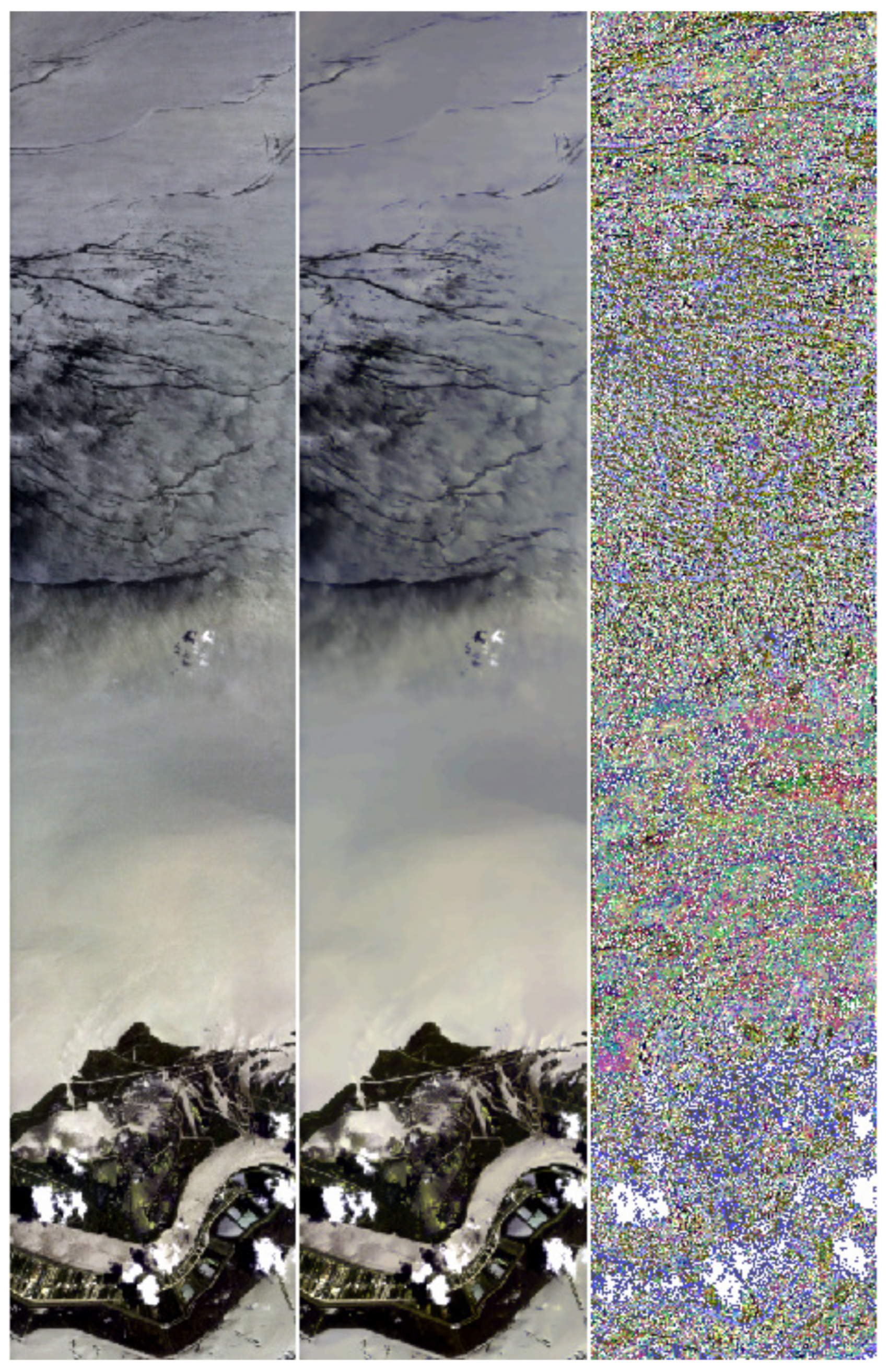
Ajka (small size). It is a resize of 400 × 256 pixels extracted from the Hyperion image (id EO1H1890272010282110KF_1R) acquired on 19 October 2010. The image shows the impact on urban and rural areas of the alumina sludge spill of a refinement factory occurred on 4 October 2010 in Ajka, Hungary (Figure 2).

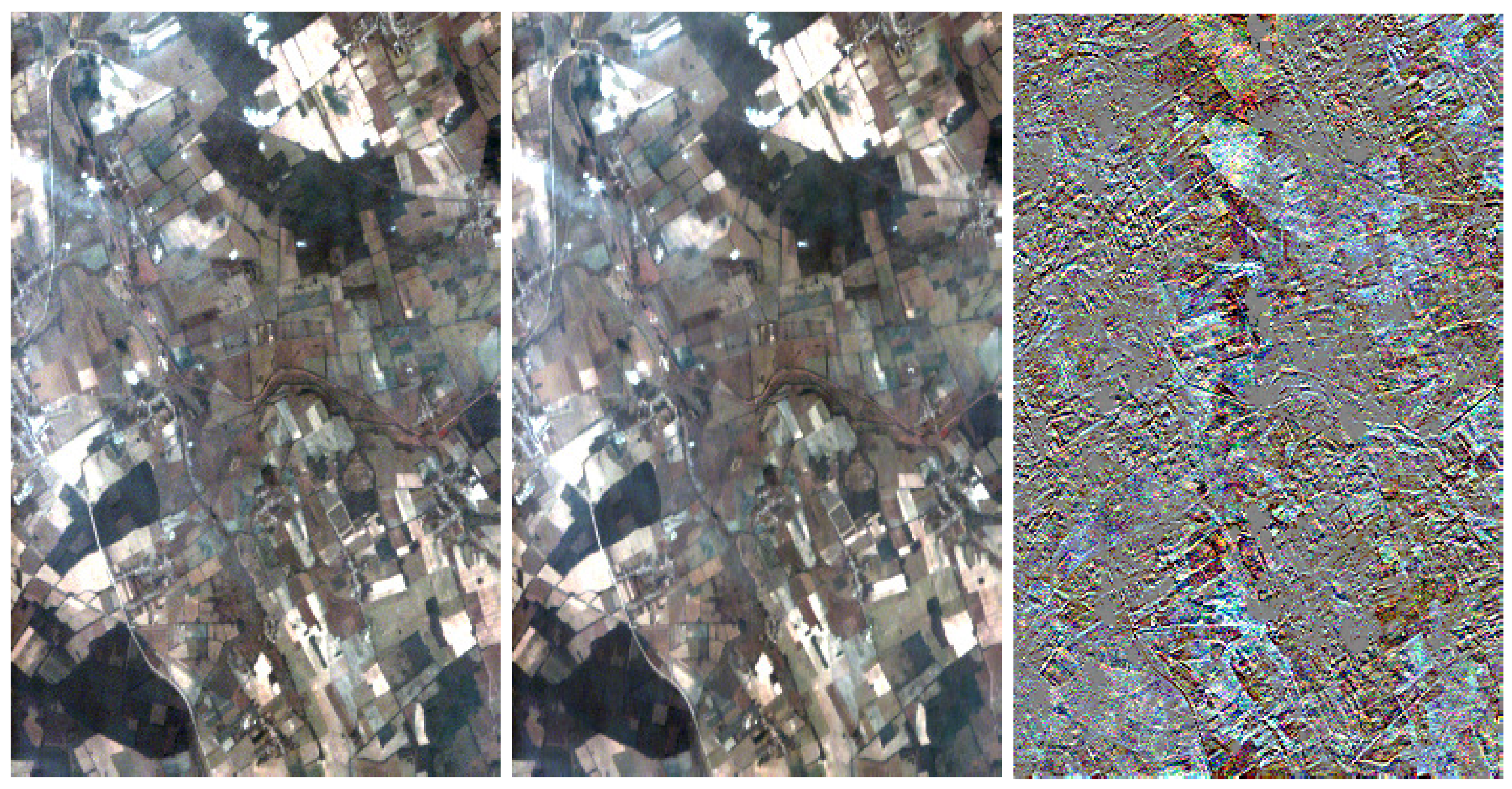
Oil Spill (medium size). It is a resize of 1200 × 256 pixels obtained by the Hyperion image (id EO1H0210402010195110KF_1R) acquired on 14 July 2010 on an area of the Gulf of Mexico (center image coordinate: 29${}^{\circ }$19${}^{\prime }$44.55${}^{\prime }$${}^{\prime }$N, 89${}^{\circ }$28${}^{\prime }$51.07${}^{\prime }$${}^{\prime }$W) interested by the huge oil-spill phenomenon occurred between April and July 2010 (Figure 3).

Desert (big size). It is an image of $6981\times 256$ pixels (id: EO1H1790412015255110P0_1R) acquired on 15 September 2015 on a uniform Egyptian desert area (center image coordinate: 27${}^{\circ }$05${}^{\prime }$01.55${}^{\prime }$${}^{\prime }$N, 25${}^{\circ }$34${}^{\prime }$48.29${}^{\prime }$${}^{\prime }$E).

4. Experiments on Hyperion Images

In this section we show the speed-up achievable with our parallel portable algorithm with respect to conventional CPU architecture in the heterogeneous platform. In particular we consider the parallel OpenCL code applied separately to the GPU and CPU platforms (therefore exploiting the parallel capabilities of both) and the serial code (working on a single core) for the CPU. As a consequence we evaluate the speed-up reachable by the parallel OpenCL code running on the GPU and the CPU with respect to the serial code running on a single-core CPU.

First of all we observe that our multi-platform portable implementation of NLM yields the same numerical results as its sequential implementation. Moreover, in order to strictly highlight performance of OpenCL, the overhead of transferring the image between the main memory of the host and the device is not included in the measured execution time.

The parallel code includes the same algorithm operations executed sequentially as shown in the Appendix A.

We compare the computational time of the parallel OpenCL algorithm for GPU and CPU of Section 2.1 with the sequential CPU code for different configurations of the NLM method in terms of search and similarity windows.

Table 2. Performance of the NLM algorithm applied to any band of the Ajka image (size $400\times 256$) for different values of the similarity (d, column 1) and search (v, column 2) windows. Computational time of the portable OpenCL code run on GPU and CPU platforms is shown in columns 3 and 5, respectively. Moreover, column 7 reports the computational time of the sequential algorithm for the CPU. The speed-up of the portable parallel algorithm with respect to the sequential one run on the GPU and on the CPU is also shown in columns 4 and 6, respectively. Cases with the highest speed-up are highlighted in boldface.

		Time	Speed-up	Time	Speed-up	Time
d	v	GPU	GPU vs. CPU	CPU (OpenCL)	CPU (OpenCL) vs. CPU	CPU
1	3	0.0006	326	0.0063	33	0.2076
2	3	0.0022	195	0.0205	21	0.4232
1	4	0.0009	383	0.0104	32	0.3312
2	4	0.0034	210	0.0367	20	0.7187
1	8	0.0025	487	0.0327	37	1.2017
2	8	0.0121	207	0.1266	20	2.5122
1	16	0.0106	460	0.11726	42	4.8737
2	16	0.0506	184	0.4603	21	9.2751
1	32	0.0364	460	0.4549	37	16.7179
2	32	0.1447	231	1.8073	19	33.3451
1	64	0.1320	500	2.0610	32	65.8862
2	64	0.4877	289	7.3622	20	140.6830
1	128	0.4214	714	7.9215	38	300.7080
2	128	1.6608	350	32.0784	19	580.3900
1	256	1.3367	798	34.1692	32	1065.4900
2	256	6.2209	361	111.8890	21	2243.2900

reports the running time of the the OpenCL parallell Algorithm 2 applied to the GPU and CPU and of the serial Algorithm 1 for CPU for size of the similarity window $d=d_x=d_y=1,2$ and of the search window $v=v_x=v_y=3,4,8,16,32,64,128,256$ for both versions of the algorithm, when relevant, for any spectral band of the Ajka image. The speed-up of the parallel algorithm on the GPU with respect to the same algorithm on the CPU and to the serial algorithm on the CPU is also shown.

Table 3. Performance of the NLM algorithms applied to any band of the Oil Spill image (size $1200\times 256$) for different values of the similarity (d, column 1) and search (v, column 2) windows. Computational time of the portable OpenCL code run on GPU and CPU platforms is shown in columns 3 and 5, respectively. Moreover, column 7 reports the computational time of the sequential algorithm for the CPU. The speed-up of the portable parallel algorithm with respect to the sequential one run on the GPU and on the CPU is also shown in columns 4 and 6, respectively. Cases with the highest speed-up are highlighted in boldface.

		Time	Speed-up	Time	Speed-up	Time
d	v	GPU	GPU vs. CPU	CPU (OpenCL)	CPU (OpenCL) vs. CPU	CPU
1	3	0.0014	415	0.0185	32	0.5846
2	3	0.0062	195	0.0591	20	1.2013
1	4	0.0021	486	0.0271	38	1.0325
2	4	0.0098	199	0.0977	20	1.9464
1	8	0.0070	497	0.0932	37	3.4612
2	8	0.0396	185	0.3554	21	7.2867
1	16	0.0295	448	0.3512	38	13.2074
2	16	0.1354	198	1.3244	20	26.7487
1	32	0.0987	504	1.2885	39	49.7303
2	32	0.3764	254	4.5136	21	95.2701
1	64	0.3437	593	5.694	36	203.94
2	64	1.3535	301	20.8591	19	406.6710
1	128	1.1533	666	23.2089	33	767.6080
2	128	5.0774	340	85.1840	20	1721.8400
1	256	4.2023	761	94.8635	34	3195.8500
2	256	19.3141	346	340.0810	20	6667.2400

and

Table 4. Performance of the NLM algorithm applied to any band of the Desert image (size $6981\times 256$) for different values of the similarity (d, column 1) and search (v, column 2) windows. Computational time of the portable OpenCL code run on GPU and CPU platforms is shown in columns 3 and 5, respectively. Moreover, column 7 reports the computational time of the sequential algorithm for the CPU. The speed-up of the portable parallel algorithm with respect to the sequential one run on the GPU and on the CPU is also shown in columns 4 and 6, respectively. Cases with the highest speed-up are highlighted in boldface.

		Time	Speed-up	Time	Speed-up	Time
d	v	GPU	GPU vs. CPU	CPU (OpenCL)	CPU (OpenCL) vs. CPU	CPU
1	3	0.0074	521	0.0791	49	3.8522
2	3	0.0421	205	0.3277	27	8.5877
1	4	0.0117	507	0.1198	50	5.9438
2	4	0.0626	199	0.4787	26	12.4373
1	8	0.0437	493	0.4614	47	21.5059
2	8	0.2280	197	1.8309	25	44.7047
1	16	0.1706	474	1.8451	44	80.7992
2	16	0.5700	295	7.2114	24	167.7810
1	32	0.4409	669	7.2103	41	294.6210
2	32	1.7229	332	26.7567	22	571.6640
1	64	1.5968	807	33.3146	39	1287.6400
2	64	7.3676	344	121.5250	21	2533.7700
1	128	6.2038	827	132.5330	39	5128.4500
2	128	30.8052	340	455.0150	23	10448.4000
1	256	24.8274	774	540.0070	36	19194.3000
2	256	117.0870	334	1990.5400	20	39105.3289

show the same results for the Oil Spill and Desert images, respectively.

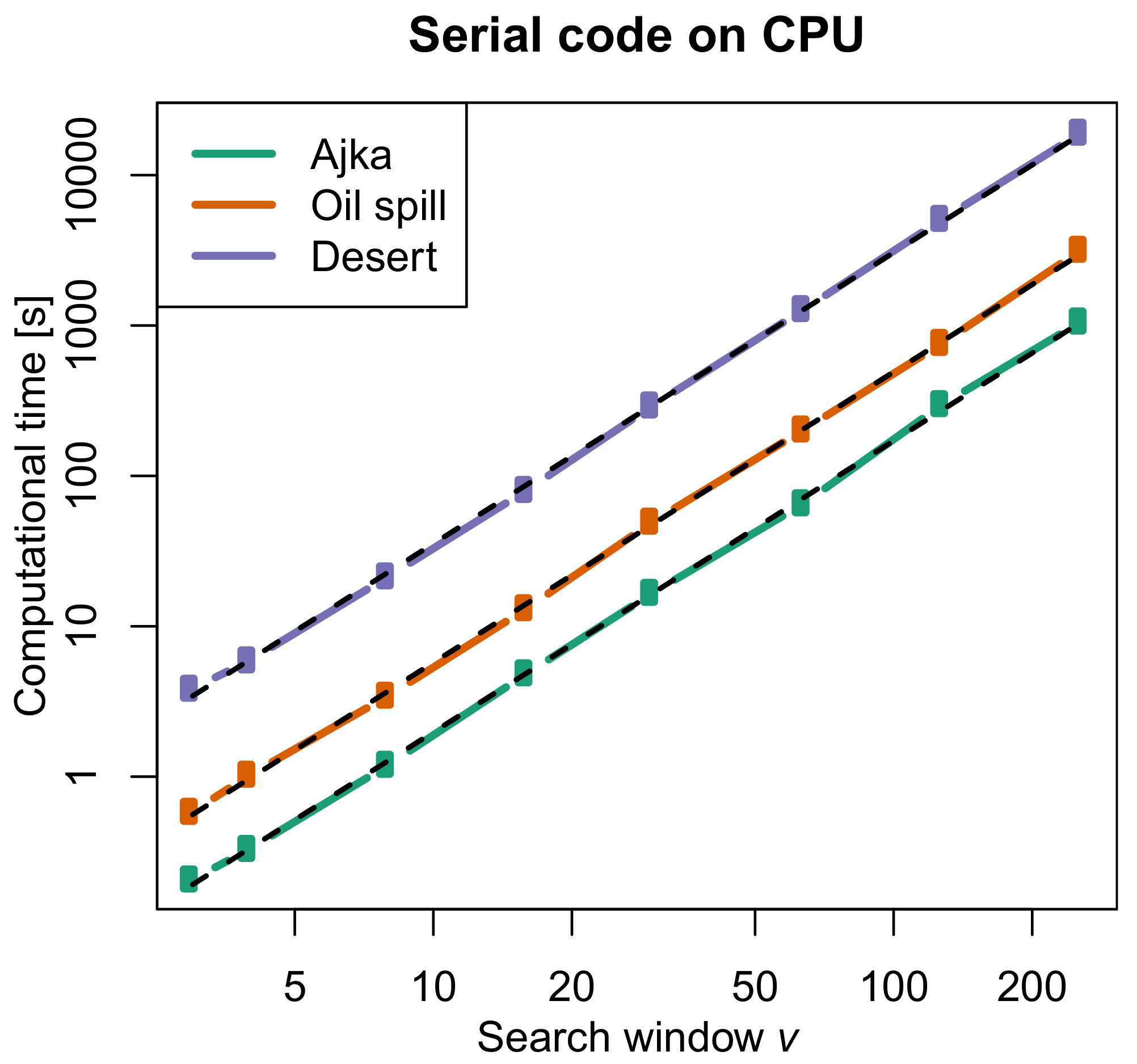
To analyze the behaviour with respect to the search window v, Figure 4 graphically shows the plot computational time vs. v of the serial algorithm for CPU for the considered images (similarity window $d=1$). Plot is given on a logarithmic scale for both axes, meaning a power relationship between computational time t and search window v as

$$t=a{v}^b;$$

(4)

the estimated exponent is $b\approx 1.94$ close to 2 and the corresponding fit is shown in the plot as a dashed line.

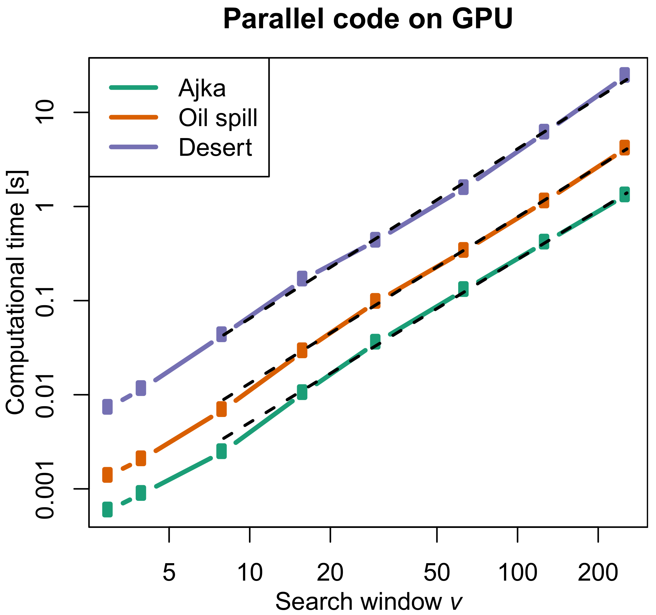
Figure 5 shows the analogous plot for the parallel algorithm on the GPU architecture. Now the estimated $b\approx 1.73-1.80<2$.

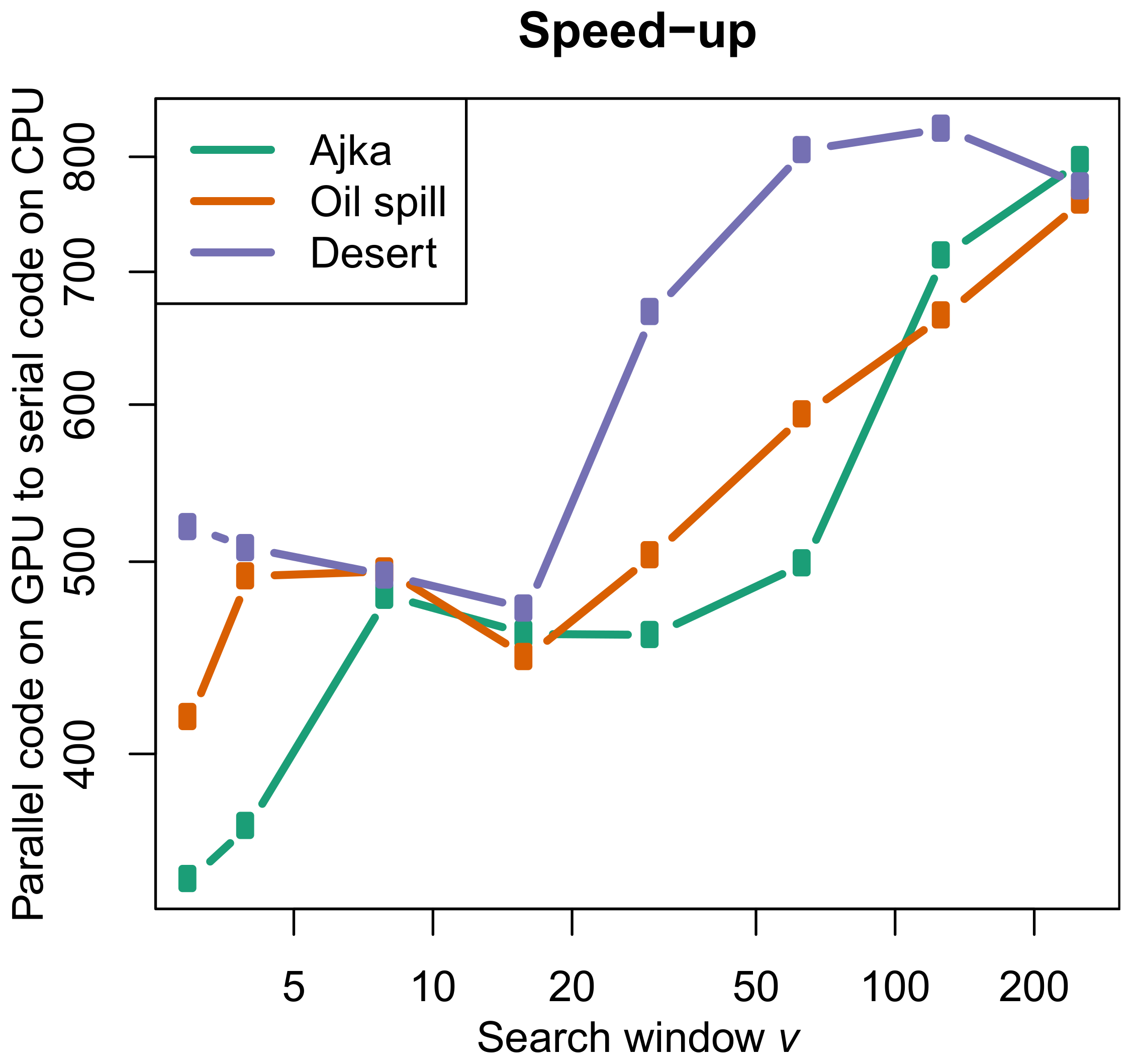
The resulting plot of speed-up of the parallel code on the GPU architecture with respect to the serial code on the CPU is shown in Figure 6.

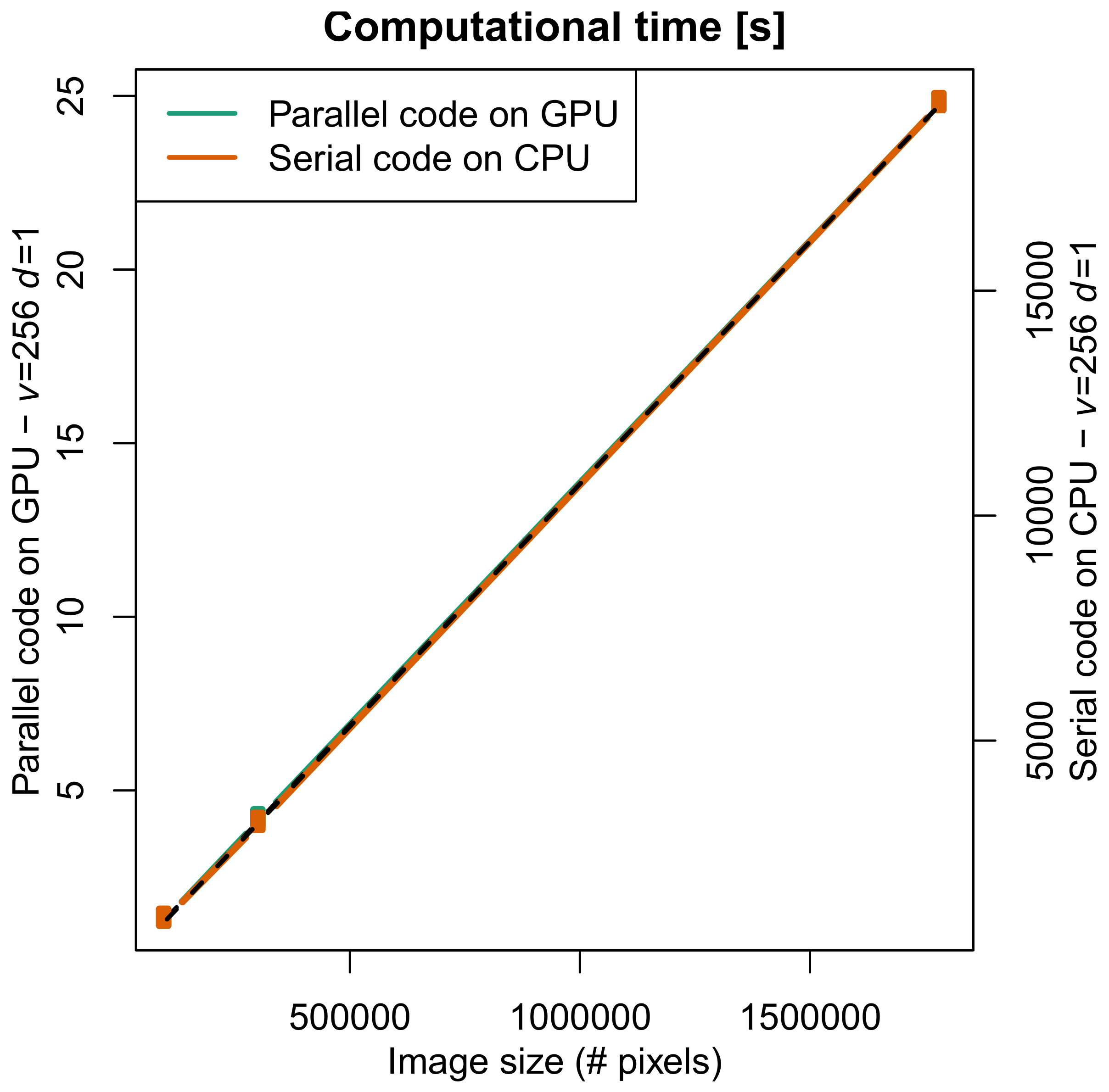
Finally to estimate dependence of the computational time on the size of the images, Figure 7 shows the computational time for CPU (left axis) and GPU (right axis) architecture in the NLM configuration $v=8$, $d=1$.

5. Results and Discussion

Table 2, Table 3 and Table 4 show that the computational time increases with d and v for all hardware configurations, as expected. Similarity window $d=1$ always yields higher speed-up than $d=2$. Instead the behaviour with respect to the search window v is more intricate. When we consider speed-up of the parallel code on the GPU architecture with respect to the serial code on the CPU we observe an irregular (often decreasing with v) behaviour up to $v=16,32$ and then a clear increase with v. This pattern depends on the size of the image. On the contrary the speed-up of the same parallel algorithm on the CPU with respect to the serial algorithm on the same CPU is much less dependent on the search window and also on the size of the image and hardware work-group size. The reason for the different behaviour is that v has better performance when is a multiple of $CL\_KERNEL\_PREFERRED\_WORK\_GROUP\_SIZE\_MULTIPLE$ due to the work-size. For example for $v=128$ there are necessary ${(128\times 2+1)}^2=66049$ threads to process the search window; this means that considering the maximum work item size of each device, they are 1024 ad 8192 for NVIDIA GPU and INTEL CPU, respectively. Then the number of work-groups used is 66,049/1024 $\approx 65$ for NVIDIA GPU with 511 idle threads and 66,049/8192 $\approx 9$ for INTEL CPU with 7679 idle threads. This observation emphasizes the importance of selecting parameters to get optimum block dimensions that are multiples of the $CL\_KERNEL\_PREFERRED\_WORK\_GROUP\_SIZE\_MULTIPLE$ size also called warp. As a consequence the configurations that yield the highest speed-up (boldface in Table 2, Table 3 and Table 4) are obtained for different values of v. In the case of speed-up of the parallel code on GPU the highest values occur for high values of v (798 at $v=256$ for the small Ajka image; 761 at $v=256$ for the medium size Oil Spill image, 827 at $v=128$ for the big Desert image) and can be considered little depending on the size. For the speed-up of the parallel code on the CPU best values are obtained for $v=16$ (42), $v=32$ (39) and $v=4$ (50) for the small, medium and large size images, respectively, that is for smaller values than the parallel code on GPU. Anyway in all configurations speed-up is never lower than 300 independently of v and size of the image for the parallel code on the GPU and 32 for the same code on the CPU.

The Tables show that our multi-platform parallel code is able to speed-up a serial code on a same CPU of a significant factor (up to 40–50). In addition we remark that the amplification factors reached are beyond the ones theoretically possible with the multicore capability of our CPU architecture (6-cores). The performance difference comes from the different architectural characteristics between CPUs and GPUs, the number of work-items and the amount of work done by a work-item that affect performance differently on CPUs and GPUs. Furthermore a huge number of work groups having a few work-items hurt performance on CPUs but help performance on GPUs. On GPUs, a single work-item is processed by a scalar processor or one single SIMD (Single Instruction Multiple Data) lane. On the contrary GPUs are specialized for supporting a large number of concurrently running threads. In addition, on CPUs the high thread-level parallelism is limited by the number of cores, so using more threads to do the same amount of work does not help performance on CPUs but hurts it due to the overhead of emulating a large number of concurrently executing work-items on a small number of cores.

We observe that the computational time for CPU based architecture increases around $2\times$ going from $d=1$ to $d=2$ for all images and search windows. On the contrary for GPU architectures the increase is somewhat higher (depending on v but systematically greater than 4); as a consequence speed-up for $d=1$ is always higher than $d=2$.

Now we specifically analyze dependence on the search window v. For CPU architecture the computational time of the serial code approximately scales as the square of v for all images, which is the value theoretically expected from the two-dimensional nature of the search window (Figure 4). The situation is different for the GPU architectures. The estimated value ($b\approx$ 1.7–1.8; Equation (4)) from Figure 5 for the parallel algorithm on the GPU indicates that the computational time increases less than quadratically with v on CPU, meaning a gain of efficiency. As a consequence the plot of speed-up of the parallel code for GPU architecture with respect to the serial code on CPU (Figure 6) is intricate but the general trend shows an increasing speed-up for large search windows (from $v=$ 16–32), whereas for small windows there is still some constant when not decrease of the speed-up with v. This behaviour can be explained with a huge number of work groups having a few work items which do not help performance on CPUs and GPUs.

Finally the even small departures of the power relationship computational time of the serial algorithm for CPU and the parallel algorithm for GPU vs. the search window lead to an intricate behaviour of the corresponding speed-up as a function of v. However the general trend of higher speed-up when the size of the image increases is clear (Figure 7).

Even though the present paper is not aimed at choosing an optimal or automatic bandwidth, nor to evaluate effectiveness of NLM as a denoising methodology compared to other competitors, Figure 2 and Figure 3 (middle) show the denoised images (Ajka and Oil Spill, respectively) obtained for the window sizes $d=2$, $v=8$. The bandwidth of the method is chosen as the standard deviation of the noise ${\sigma }_i$ for each spectral channel $i=1,\dots ,242$. ${\sigma }_i$ is estimated starting from the available characteristics of the Hyperion SNR [2] basing on the actual signal strength of the images. As a rule-of-the-thumb the windows sizes ($d=2$, $v=8$) have been chosen for these images, as we observe a negligible difference in the denoised images using larger windows. For images from other sensors with a different SNR the choice of d and v could be based on different arguments. We remark again that the computational time does not depend on bandwidth h. Finally Figure 2 (right) shows the noise estimated by NLM composing the three difference images at the same RGB spectral bands for the Ajka image.

6. Conclusions

We have developed a multi-platform algorithm for denoising remotely sensed images for CPU and GPU architectures. A major benefit of using an OpenCL algorithm is that the same kernel can be easily executed on different platforms as shown. It is able to dramatically speed-up computational time by a factor ranging from around $300\times$ to $700\times$ depending on the size of the search window and of the image with respect to traditional serial C++ algorithms on CPU. In addition the very same algorithm, when run on commodity CPU, is already able to boost computational performance by a factor up to 40–50 depending on the search window and on the size of the image.

As a consequence NLM, known in the literature as a very effective yet time consuming methodology for denoising images, becomes a viable way to denoise remotely sensed images in real-time; furthermore it makes time consuming tuning bandwidth very fast. Moderate cost of the GPU technology and continuous progress in its architecture are fast spreading its use within the remote sensing community. The proposed algorithm can serve as a firm basis for ongoing and future upgrades of portable multi-platforms algorithms.

References

- Green, R.O.; Eastwood, M.L.; Sarture, C.M.; Chrien, T.G.; Aronsson, M.; Chippendale, B.J.; Faust, J.A.; Pavri, B.E.; Chovit, C.J.; Solis, M.; et al. Imaging spectroscopy and the airborne visible/infrared imaging spectrometer (AVIRIS). Remote Sens. Environ. 1998, 65, 227–248. [Google Scholar] [CrossRef]
- Pearlman, J.; Segal, C.; Liao, L.B.; Carman, S.L.; Folkman, M.A.; Browne, W.; Ong, L.; Ungar, S.G. Development and operations of the EO-1 Hyperion imaging spectrometer. In Proceedings of the International Symposium on Optical Science and Technology, SPIE 4135, Earth Observing Systems V, San Diego, CA, USA, 30 July–4 August 2000; p. 8. [Google Scholar] [CrossRef]
- Pignatti, S.; Acito, N.; Amato, U.; Casa, R.; de Bonis, R.; Diani, M.; Laneve, G.; Matteoli, S.; Palombo, A.; Pascucci, S.; et al. Development of algorithms and products for supporting the Italian hyperspectral PRISMA mission: The SAP4PRISMA project. In Proceedings of the 2012 IEEE International Geoscience and Remote Sensing Symposium, Munich, Germany, 22–27 July 2012; pp. 127–130. [Google Scholar] [CrossRef]
- Hilton, F.; Armante, R.; August, T.; Barnet, C.; Bouchard, A.; Camy-Peyret, C.; Capelle, V.; Clarisse, L.; Clerbaux, C.; Coheur, P.-F.; et al. Hyperspectral earth observation from IASI: Five years of accomplishments. Bull. Amer. Meteor. Soc. 2012, 93, 347–370. [Google Scholar] [CrossRef]
- Rodriguez, A.; Stuhlmann, R.; Tjemkes, S.; Aminou, D.M.; Stark, H.; Blythe, P. Meteosat Third Generation: mission and system concepts. In Proceedings of the SPIE Conference on Optical Engineering + Applications, SPIE 7453, Infrared Spaceborne Remote Sensing and Instrumentation, XVII, San Diego, CA, USA, 24–27 June 2009; p. 10. [Google Scholar] [CrossRef]
- Masiello, G.; Serio, C. Dimensionality-reduction approach to the thermal radiative transfer equation inverse problem. Geophys. Res. Lett. 2004, 31, L11105/11. [Google Scholar] [CrossRef]
- Amato, U.; Antoniadis, A.; De Feis, I.; Masiello, G.; Matricardi, M.; Serio, C. Technical note: Functional sliced inverse regression to infer temperature, water vapour and ozone from IASI data. Atm. Chem. Phys. 2009, 9, 5321–5330. [Google Scholar] [CrossRef] [Green Version]
- Masiello, G.; Serio, C.; Antonelli, P. Inversion for atmospheric thermodynamical parameters of IASI data in the principal components space. Q. J. R. Met. Soc. 2012, 138, 103–117. [Google Scholar] [CrossRef] [Green Version]
- Serio, C.; Masiello, G.; Liuzzi, G. Demonstration of random projections applied to the retrieval problem of geophysical parameters from hyper-spectral infrared observations. Appl. Opt. 2016, 55, 6576–6587. [Google Scholar] [CrossRef]
- Amato, U.; Antoniadis, A.; Cuomo, V.; Cutillo, L.; Franzese, M.; Murino, L.; Serio, C. Statistical cloud detection from SEVIRI multispectral images. Remote Sens. Environ. 2008, 112, 750–766. [Google Scholar] [CrossRef]
- Amato, U.; Lavanant, L.; Liuzzi, G.; Masiello, G.; Serio, C.; Stuhlmann, R.; Tjemkes, S.A. Cloud mask via cumulative discriminant analysis applied to satellite infrared observations: scientific basis and initial evaluation. Atmos. Meas. Tech. 2004, 7, 3355–3372. [Google Scholar] [CrossRef]
- Báscones, D.; González, C.; Mozos, D. Hyperspectral Image Compression Using Vector Quantization, PCA and JPEG2000. Remote Sens. 2018, 10, 907. [Google Scholar] [CrossRef] [Green Version]
- Christophe, E.; Michel, J.; Inglada, J. Remote sensing processing: From multicore to GPU. IEEE J. Sel. Top. Appl. Earth Obs. Remote Sens. 2011, 4, 643–652. [Google Scholar] [CrossRef]
- Liu, Y.; Chen, B.; Yu, H.; Zhao, Y.; Huang, Z.; Fang, Y. Applying GPU and POSIX thread technologies in massive remote sensing image data processing. In Proceedings of the IEEE 19th International Conference on Geoinformatics, Dhanghai, China, 24–26 June 2009. [Google Scholar] [CrossRef]
- Ma, Y.; Chen, L.; Liu, P.; Lu, K. Parallel programing templates for remote sensing image processing on GPU architectures: design and implementation. Computing 2016, 98, 7–33. [Google Scholar] [CrossRef]
- Wu, X.; Huang, B.; Plaza, A.; Li, Y.; Wu, C. Real-time implementation of the pixel purity index algorithm for endmember identification on GPUs. IEEE Geosci. Remote Sens. Lett. 2014, 11, 955–959. [Google Scholar] [CrossRef]
- Agathos, A.; Li, J.; Petcu, D.; Plaza, A. Multi-GPU implementation of the minimum volume simplex analysis algorithm for hyperspectral unmixing. IEEE J. Sel. Top. Appl. Earth Obs. Remote Sens. 2014, 7, 2281–2296. [Google Scholar] [CrossRef]
- Torti, E.; Acquistapace, M.; Danese, G.; Leporati, F.; Plaza, A. Real-Time Identification of Hyperspectral Subspaces. IEEE J. Sel. Top. Appl. Earth Obs. Remote Sens. 2014, 7, 2680–2687. [Google Scholar] [CrossRef]
- Wu, Z.; Ye, S.; Liu, J.; Sun, L.; Wei, Z. Sparse non-negative matrix factorization on GPUs for hyperspectral unmixing. IEEE J. Sel. Top. Appl. Earth Obs. Remote Sens. 2014, 7, 3640–3649. [Google Scholar] [CrossRef]
- Nascimento, J.M.; Bioucas-Dias, J.M.; Rodriguez Alves, J.M.; Rodriguez Alves, J.M.; Silva, V.M.; Plaza, A. Parallel hyperspectral unmixing on GPUs. IEEE Geosci. Remote Sens. Lett. 2014, 11, 666–670. [Google Scholar] [CrossRef]
- Mei, S.; He, M.; Shen, Z. Optimizing Hopfield neural network for spectral mixture unmixing on GPU platform. IEEE Geosci. Remote Sens. Lett. 2014, 11, 818–822. [Google Scholar] [CrossRef]
- Lei, Z.; Wang, M.; Li, D.; Lei, T.L. Stream model-based orthorectification in a GPU cluster environment. IEEE Geosci. Remote Sens. Lett. 2014, 11, 2115–2119. [Google Scholar] [CrossRef]
- Passerone, C.; Sansoe, C.; Maggiora, R.; Volio, A.C.; Zavagli, M.; Minati, F.; Costantini, M. Highly parallel image co-registration techniques using GPUs. In Proceedings of the 2014 IEEE Aerospace Conference, Big Sky, MT, USA, 1–8 March 2014. [Google Scholar] [CrossRef]
- Alvarez-Cedillo, J.; Herrera-Lozada, J.; Rivera-Zarate, I. Implementation strategy of NDVI algorithm with Nvidia Thrust. In Image and Video Technology; Springer: Berlin/Heidelberg, Germany, 2014; pp. 184–193. [Google Scholar] [CrossRef]
- López-Fandiño, J.; Quesada-Barriuso, P.; Heras, D.B.; Argüello, F. Efficient ELM-Based Techniques for the Classification of Hyperspectral Remote Sensing Images on Commodity GPUs. IEEE J. Sel. Top. Appl. Earth Obs. Remote Sens. 2015, 8, 2884–2893. [Google Scholar] [CrossRef]
- Bernabé, S.; López, S.; Plaza, A.; Sarmiento, R. GPU implementation of an automatic target detection and classification algorithm for hyperspectral image analysis. IEEE Geosci. Remote Sens. Lett. 2013, 10, 221–225. [Google Scholar] [CrossRef]
- Falcao, G.; Silva, V.; Sousa, L.; Andrade, J. Portable LDPC Decoding on Multicores Using OpenCL [Applications Corner]. IEEE Signal Process. Mag. 2012, 29, 81–109. [Google Scholar] [CrossRef]
- Bernabé, S.; García, C.; Igual, F.D.; Botella, G.; Prieto-Matia, M.; Plaza, A. Portability Study of an OpenCL Algorithm for Automatic Target Detection in Hyperspectral Images. IEEE Trans. Geosci. Remote. Sens. 2019, 57, 9499–9511. [Google Scholar] [CrossRef]
- Fang, L.; Wang, M.; Ying, H.; Hu, F. Multi-GPU based near real-time preprocessing and releasing system of optical satellite images. In Proceedings of the 2014 IEEE International Geoscience and Remote Sensing Symposium (IGARSS), Quebec City, QC, Canada, 13–18 July 2014. [Google Scholar] [CrossRef]
- Castro-Palazuelos, D.; Robles-Valdez, D.; Torres-Roman, D. An Efficient GPU-Based Implementation of the R-MSF-Algorithm for Remote Sensing Imagery. In Progress in Pattern Recognition, Image Analysis, Computer Vision, and Applications, Proceedings of the 19th Iberoamerican Congress, CIARP 2014, Puerto Vallarta, Mexico, 2–5 November 2014; Springer: Cham, Switzerland, 2014. [Google Scholar] [CrossRef] [Green Version]
- Quesada-Barriuso, P.; Argüello, F.; Heras, D.B.; Benediktsson, J.A. Wavelet-Based Classification of Hyperspectral Images Using Extended Morphological Profiles on Graphics Processing Units. IEEE J. Sel. Top. Appl. Earth Obs. Remote Sens. 2015, 8, 2962–2970. [Google Scholar] [CrossRef]
- Gilbert Serra, X.; Patel, V.M.; Labate, D.; Chellappa, R. Discrete shearlet transform on GPU with applications in anomaly detection and denoising. EURASIP J. Adv. Signal Process. 2014, 64, 1–14. [Google Scholar] [CrossRef]
- Jihua, T.; Jinping, S.; Yuxi, Z.; Ahmad, N.; Bingchen, Z. Parallel Implementation of Compressive Sensing Based SAR Imaging with GPU. J. Converg. Inf. Technol. 2011, 6, 122–128. [Google Scholar]
- Ozcan, C.; Sen, B.; Nar, F. GPU efficient SAR image despeckling using mixed norms. In Proceedings of the SPIE Remote Sensing 2014, Amsterdam, The Netherlands, 22–25 September 2014. [Google Scholar] [CrossRef]
- Dolwithayakul, B.; Chantrapornchai, C.; Chumchob, N. Additive and Multiplicative Noise Removal Framework for Large Scale Color Satellite Images on OpenMP and GPUs. Stud. Surv. Mapp. Sci. 2013, 1, 10–16. [Google Scholar]
- Buades, A.; Coll, B.; Morel, J.M. A review of image denoising algorithms, with a new one. SIAM J. Multiscale Model. Simul. 2005, 4, 490–530. [Google Scholar] [CrossRef]
- Shi, Y.; Zhu, X.; Bamler, R. Optimized parallelization of non-local means filter for image noise reduction of InSAR image. In Proceedings of the 2015 IEEE International Conference on Information and Automation, Lijiang, China, 8–10 August 2015. [Google Scholar] [CrossRef]
- Xue, B.; Huang, Y.; Yang, J.; Shi, L.; Zhan, Y.; Cao, X. Fast nonlocal remote sensing image denoising using cosine integral images. IEEE Geosci. Remote Sens. Lett. 2013, 10, 1309–1313. [Google Scholar] [CrossRef]
- Deledalle, C.A.; Denis, L.; Tupin, F.; Reigber, A.; Jäger, M. NL-SAR: A unified nonlocal framework for resolution-preserving (Pol)(In) SAR Denoising. IEEE Trans. Geosci. Remote Sens. 2015, 53, 2021–2038. [Google Scholar] [CrossRef] [Green Version]
- Kharlamov, A.; Podlozhnyuk, V. Image Denoising; Technical Report NVIDIA; NVIDIA Corp.: Santa Clara, CA, USA, 2007. [Google Scholar]
- Márques, A.; Pardo, A. Implementation of Non Local Means Filter in GPUs. In Progress in Pattern Recognition, Image Analysis, Computer Vision, and Applications. CIARP 2013; CIARP 2013. Lecture Notes in Computer Science, Vol. 8258; Ruiz-Shulcloper, J., Sanniti di Baja, G., Eds.; Springer: Berlin/Heidelberg, Germany, 2013. [Google Scholar] [CrossRef] [Green Version]
- Palma, G.; Comerci, M.; Alfano, B.; Cuomo, S.; De Michele, P.; Piccialli, F.; Borrelli, P. 3D Non-Local Means denoising via multi-GPU. In Proceedings of the 2013 Federated Conference on Computer Science and Information Systems, Kraków, Poland, 8–11 September 2013. [Google Scholar]
- Cuomo, S.; De Michele, P.; Piccialli, F. 3D Data Denoising via Nonlocal Means Filter by Using Parallel GPU Strategies. Comp. Math. Meth. Med. 2014, 2014, 523862. [Google Scholar] [CrossRef] [Green Version]
- Zimmer, A.; Ghuman, P. CUDA Optimization of Non-local Means Extended to Wrapped Gaussian Distributions for Interferometric Phase Denoising. Procedia Comp. Sci. 2016, 80, 166–177. [Google Scholar] [CrossRef] [Green Version]
- Efros, A.; Leung, T. Texture synthesis by non-parametric sampling. In Proceedings of the Seventh IEEE International Conference on Computer Vision, Kerkyra, Greece, 20–27 September 1999; pp. 1033–1038. [Google Scholar] [CrossRef] [Green Version]
- Manjón, J.V.; Coupé, P.; Martí-Bonmatí, L.; Collins, D.L.; Robles, M. Adaptive non-local means denoising of MR images with spatially varying noise levels. J. Magn. Reson. Imaging 2010, 31, 192–203. [Google Scholar] [CrossRef] [PubMed] [Green Version]
Figure 1.
Open Computing Language (OpenCL) runtime functions supporting the parallel execution of NonLocal Means (NLM) kernel using threaded blocks.
Figure 2.
Original (left) and NLM denoised (middlke) RGB Ajka image. Difference of the two images (estimated noise) is shown on the right composing the differences of the same RGB bands.
Figure 3.
Original (left) and NLM denoised (middle) RGB Oil Spill image. Difference of the two images (estimated noise) is shown on the right composing the differences of the same RGB bands.
Figure 4.
Plot of the computational time of the serial algorithm for CPU vs. search window v (similarity window ). Curves refer to the Ajka, Oil Spill and Desert images. The fit by Equation (4) is also shown as a dashed line.
Figure 5.
Plot of the computational time of the parallel algorithm on the GPU vs. search window v (similarity window ). Curves refer to the Oil Spill, Desert and Ajka images. The fit by Equation (4) is also shown as a dashed line.
Figure 6.
Plot speed-up of the parallel code on the GPU architecture with respect to the serial code on the CPU vs. search window v (similarity window ) for images Oil Spill, Desert, Ajka.
Figure 7.
Plot computational time vs. size of the images (number of pixels) for 1 GPU unit and CPU architectures (case , ). Corresponding regression fit is shown as black dashed lines.