Mapping Growing Stem Volume of Chinese Fir Plantation Using a Saturation-based Multivariate Method and Quad-polarimetric SAR Images

Abstract

For the planning and sustainable management of forest resources, well-managed plantations are of great significance to mitigate the decrease of forested areas. Monitoring these planted forests is essential for forest resource inventories. In this study, two ALOS PALSAR-2 quad-polarimetric synthetic aperture radar (SAR) images and ground measurements were employed to estimate growing stem volume (GSV) of Chinese fir plantations located in a hilly area of southern China. To investigate the relationships between forest GSV and polarization characteristics, single and fused variables were derived by the Yamaguchi decomposition and the saturation value of GSV was estimated using a semi-exponential empirical model as a base model. Based on the estimated saturation values and relative root mean square error (RRMSE), the single and fused characteristics and corresponding models were selected and integrated, which led to a novel saturation-based multivariate method used to improve the GSV estimation and mapping of Chinese fir plantations. The new findings included: (1) All the original polarimetric characteristics, statistically, were not significantly correlated with the forest GSV, and their logarithm and ratio transformation fused variables greatly improved the correlations, thus the estimation accuracy of the forest GSV. (2) The logarithm transformation of surface scattering resulted in the greatest saturation, value but the logarithm transformation of double-bounce scattering resulted in the smallest RRMSE of the GSV estimates. (3) Compared with the single transformations, the fused variables led to more reasonable saturation values and obviously reduced the values of RRMSE. (4) The saturation-based multivariate method led to more accurate estimates of the forest GSV than the univariate method, with the smallest value (29.64%) of RRMSE achieved using the set of six variables. This implied that the novel saturation-based multivariate method provided greater potential to improve the estimation and mapping of the forest GSV.

1. Introduction

Through carbon sequestration and biomass accumulation, planted forests play a major role in mitigation of global climate change, due to the reduction of natural forests and increase of plantations during the past four decades. However, it is often difficult to directly obtain forest above ground biomass (AGB) for large areas. Rather than what is done for natural forests, instead, the AGB of plantations is usually derived by first measuring tree heights and diameters at breast height and calculating tree growing stem volumes (GSV) using allometric equations and then multiplying GSV with biomass expansion factors; that is, gravity coefficients by tree species. Thus, GSV is a basic and key factor in the planning and sustainable management of planted forest resources at regional scales [1,2,3].

However, GSV is often obtained by ground measurements by sampling, which is time-consuming, labor-intensive and costly [4,5]. The topographic complexity of mountainous regions makes the ground-based survey even more difficult and costly. Remote sensing images have been widely used to map GSV on regional scales by combining them with field measurements of GSV at plot level. Because of the impacts of clouds, fogs and moisture, it is very hard to acquire adequate optical images for estimation of forest GSV in southern China, in which there is a subtropical monsoon climate. For that purpose, microwave remote sensing imagery that is less affected by clouds, fogs and moisture bears significant potential. Moreover, synthetic aperture radar (SAR) data coupled with quad-polarimetric techniques have a stronger ability to account for the propagation and scattering mechanism than the single polarimetric SAR images [6]. With the capacity to penetrate forest canopies and interact with forest structures, quad-polarimetric SAR images provide great potential to improve the accuracy of forest GSV monitoring and assessment [6,7,8,9].

Polarimetric characteristics that are highly sensitive to forest GSV can be used to accurately estimate forest GSV [6,7,8,10,11]. There are three kinds of polarimetric characteristics associated with forest GSV. The first one is the trio of backscattering coefficients—horizontal-horizontal (HH), horizontal-vertical (HV) and vertical-vertical (VV) [7,8,12,13]. The backscattering coefficients of the dual and quad-polarization SAR images have been proved to be appropriate for estimating forest GSV [7,8,11,12,13,14,15,16,17]. The second one is the coherence of SAR interferometry (InSAR) with different bands and polarizations [11,12,18,19,20,21,22,23]. The last one is the multiple features derived by polarimetric decomposition [24,25,26,27,28,29,30,31]. There are often strong correlations between the powers of decomposition components and forest GSV [27,28,29,30,31]. Polarimetric SAR images provide plenty of independent variables that can be used to estimate forest GSV, but most of the models employ only one kind of polarimetric characteristic and ignore other polarimetric properties related to forest structure parameters. How to integrate the related polarimetric characteristics becomes meaningful to improve forest GSV estimation accuracy.

The three kinds of polarimetric characteristics have been successfully used to estimate GSV of different forests. However, without physical meaning related to scatterings, the backscattering coefficients from different polarizations become saturated at certain levels of GSV [10,11]. It is also well known that the coherence of InSAR has great potential to map forest parameters, but the approach requires two appropriate SAR images related to a temporal baseline, spatial baseline and environmental conditions [18,19,20,21,22,23]. The polarimetric decomposition theorem has been developed to extract physical parameters from SAR images without any ground measurements. Several decomposition approaches have been proposed, including the Cloude decomposition, Freeman three-component decomposition and Yamaguchi four-component decomposition [24,25,26,27,28]. The Cloude decomposition has been commonly used and continuously improved for target classification [24,25]. The Freeman decomposition is developed based on the three-component scattering model related to the surface, double-bounce and volume scatterings [24,25,26,27]. Based on Freeman decomposition, Yamaguchi proposed a four-component scattering model by introducing an additional term, helix scattering, for non-reflection symmetric cases [24,25,28,29,30,31,32]. Different from the Freeman decomposition, the Yamaguchi decomposition takes into account the modification of the volume scattering matrix and decreases the mistakes for distinguishing the volume scattering from double-bounce scattering. With the explicitly physical property related to scattering, the scattering components from Yamaguchi decomposition are more suitable for mapping forest parameters [28,29,30,31,32].

Furthermore, polarimetric characteristics become saturated at a certain GSV level, which means that the polarimetric properties are not sensitive to the changes of forest GSV after a certain value [9,20,21,22]. Analyzing the saturation levels of the polarimetric characteristics, therefore, has great potential to improve the mapping accuracy of forest GSV [9,31]. Both parametric and non-parametric methods (

Table 1. Previous studies investigating the potential of growing stem volume (GSV) saturation using synthetic aperture radar (SAR) images.

Authors	Data	Area	Forest Type	Model	Saturation (m3/ha)	RMSE (m3/ha)	RRMSE (%)
Santoro (2002) [18]	C-band ERS-1/2 (coherence)	Sweden	Boreal coniferous,	Semi-Empirical Model	Max: 350	Min:22 Max:152	Not estimated
Santoro (2006) [14]	L-band JERS-1 (backscatter)	Sweden, Finland Siberia	Boreal coniferous,	Semi-Empirical Model	Min: 100 Max: 300	Min: 36 Max: 152	Min: 25% Max:68%
Pulliainen (2003) [35]	C band ERS-1/2 (coherence)	Finland	Norway spruce/Scots pine	Semi-Empirical Model	Not estimated	Not estimated	Max:48%
Askne (2005) [34]	C band ERS-1/2 (coherence)	Finland	boreal coniferous species	Semi-Empirical Model Interferometric HUT Model	Not estimated	Not estimated	Not estimated
Antropov (2013) [10]	ALOS PALSAR dual polarization (backscatter)	Finland	mixed forest.	Semi-Empirical Model	150–200	Min: 40 Max: 66	Min: 42% Max:63%
Chowdhury (2013) [7]	ALOS PALSAR Quad polarization (backscatter)	Central Siberia	mixed forest.	Semi-Empirical Model	Min: 80 Max: 595	Not estimated	Not estimated
Chowdhury (2014) [20]	ALOS PALSAR Quad polarization (coherence)	Central Siberia	mixed forest.	Semi-Empirical Model	250	Min: 33 Max: 42	Not estimated

) have been employed to detect the saturation levels [7,8,9,10,12,13,14,15,16,17,18,19,20,32,33,34,35]. The non-parametric methods mean that the saturation values can be indirectly retrieved by visually interpreting the extreme values of linear models and the trends of nonlinear models [14,16,36,37]. For example, Gonçalves et al. [36] and Abdullahi et al. [37] obtained the GSV saturation levels exceeding 300 m³/ha for tropical forests and complex temperate forests using the extreme values of a linear model. But, determining the extreme values is not easy and accurate. A semi-exponential model derived from the simplified water cloud model (WCM) is one of the parametric methods in which the saturation level is considered as one of parameters in the model [20,21,22,23,31,34,35,36,37,38,39]. Then, the saturation values are directly solved by non-linear algorithms with initial values of parameters provided [14,38,39,40]. The saturation levels vary with polarimetric characteristics because of different sensitivities to forest GSV. The selected independent variable with a low saturation level makes it hard to estimate the values of forest GSV that exceed the saturation level. On the other hand, taking advantage of different polarimetric characteristics and accurately capturing the saturation levels would help to improve the accuracy for estimating forest GSV.

The previous studies of using SAR images to determine the saturation values and estimate GSV mainly focused on the use of semi-empirical models and boreal and natural forests (Table 1), and the obtained saturation values of GSV varied from 80 to 595 m³/ha. There have been very few reports that dealt with planted forests. The area of planted forests in China ranks the highest in the world. Chinese fir is the top tree species out of the plantations in China and distributed in more than 10 provinces located in the East, Southeast, South and central south, and southwestern parts of China. Thus, Chinese fir is the most important species for wood supply in China and its contribution to sustainable forest ecosystems and global carbon cycling is also very significant. There have been few studies to explore the saturation of GSV using SAR and optical images for estimation of Chinese fir forest biomass and GSV. The planted Chinese fir forests have complicated and different canopy structures from other species because of different climatic, topographic and soil properties. Determining the saturation values of GSV and accurately deriving its spatial distribution become very important.

The previous methods for mapping GSV of Chinese fir plantations have concentrated on the use of multi-source remote sensing data, but using quad-polarimetric SAR images has been rarely reported [41,42,43]. In this study, two ALOS PALSAR-2 quad-polarimetric SAR images acquired on June 30 and August 25 in 2016 were selected to estimate the GSV values of Chinese fir plantations located in a hilly area of southern China. We analyzed and compared the single and fused polarimetric characteristics to interpret forest structure parameters and estimate the saturation levels using the aforementioned semi-exponential empirical model as a base model. We then developed a novel saturation-based multivariate method in which the saturation values were considered as a model parameter and the saturation-based models with different characteristics and saturation levels were selected and integrated to map the forest GSV of the study area.

The paper was organized as follows. Section 2 introduced the study area and data from the measured plots and the acquired quad-polarimetric SAR images. The polarimetric SAR data pre-processing and the methods for estimating the saturation levels and mapping forest GSV were demonstrated in Section 3. In Section 4, the results of the saturation levels and the forest GSV estimated by the univariate and multivariate methods were compared. The factors affecting the saturation levels and the estimation accuracy of forest GSV were discussed in Section 5 and the conclusions were drawn in Section 6.

2. Study Area and Datasets

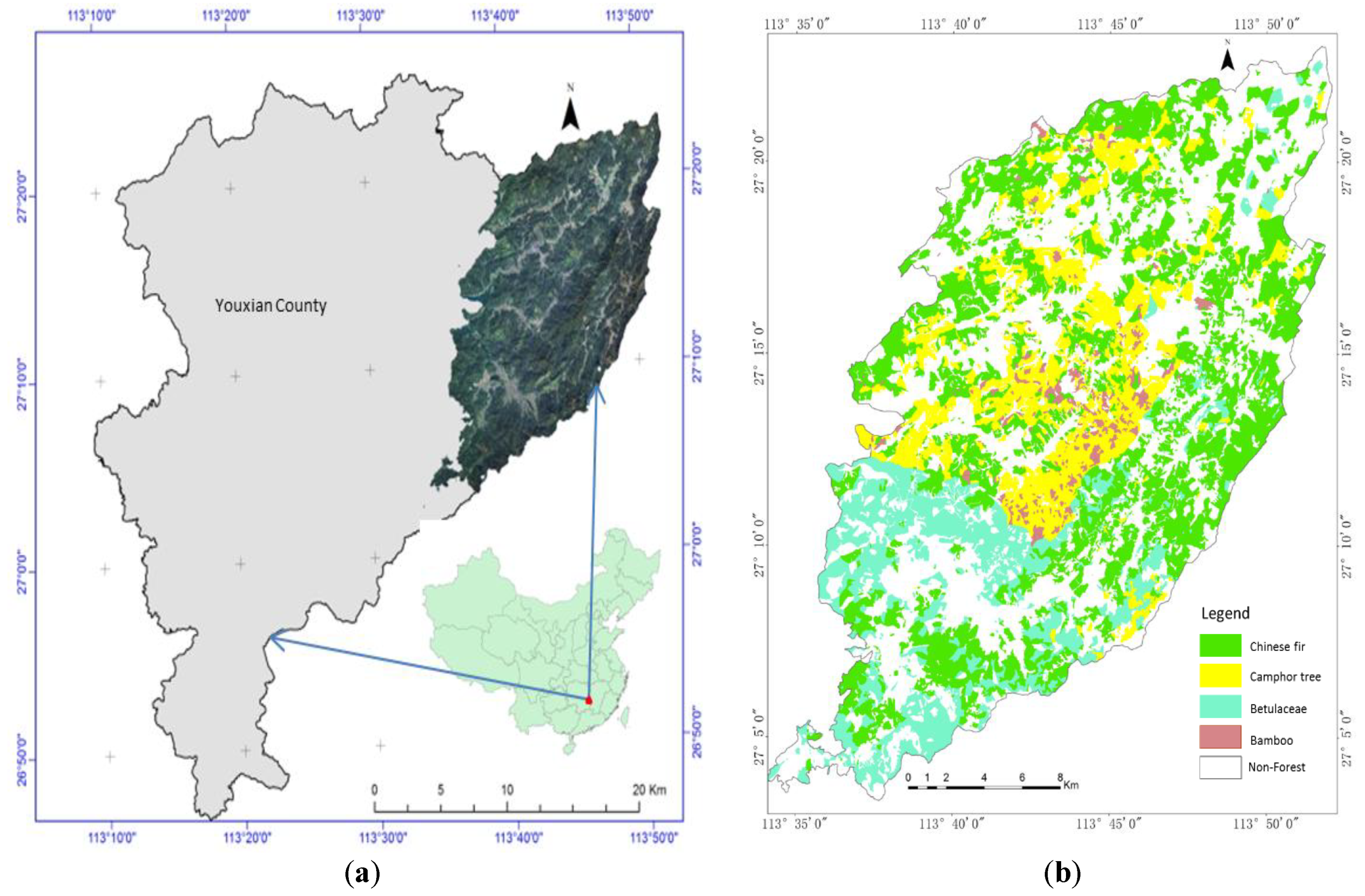
2.1. Study Area

This study was conducted in the Huangfengqiao state-owned forest farm in Youxian county (113°24′ N, 27°15′ E), Hunan province of China (Figure 1a). The study area has a hilly landscape with the elevation varying from 115 m to 1270 m and a slope ranging from 20 to 35 degrees. Located in the subtropical monsoon climate zone, this area has an annual average temperature of 17.8 °C, an average precipitation of 1410.8 mm and an average frost-free period of 292 days. About 86.24% of the region (10,122.6 ha) is covered by Chinese fir (Cunninghamia Lanceolata), Pinus massoniana Lamb, bamboo, Liriodendron chinense and Cinnamomum camphora. The planted Chinese fir is dominant species in the hilly terrain (Figure 1b).

2.2. Ground Data Collection and Processing

Most Chinese fir plantations were distributed in the northern and eastern parts of the study area. By the approach of random stratification sampling based on the spatial distribution of the Chinese fir plantations and age groups, a total of 50 plots were measured from 2016 to 2017 (Figure 2a) and as examples, the photos in Figure 2b showed three ground measured plots with young, immature and mature forests. The random stratification sampling led to the sample plots that had a consistent spatial distribution with that of the Chinese fir plantations in the study area (Figure 1b versus Figure 2a). All the sample plots were pure Chinese fir plantation forests. There were only 6 sample plots in which Chinese fir was mixed with broad-leaved tree species and Masson pine, but the percentages of broad-leaved tree species and Masson pine were less than 8%. The ground measured plot GSV values were used to investigate the relationship between polarimetric characteristics and the Chinese fir forest GSV. The plots had a size of 30 m × 30 m or 20 m × 20 m depending on the topographic features. The locations of the selected plots, including the corners and central points, were accurately obtained using the real-time dynamic measurement (RTK) global positioning system (GPS). In each plot, the height and the diameter at breast height (DBH) of each tree were measured. Trees with the DBH equal to or greater than 5 cm were considered in the inventory.

In each plot, the stem volume of the i-th tree was estimated by:

$$V_i=g_i\times (H_i+3)\times f_{\epsilon }$$

(1)

in which $V_i$ is the stem volume, $g_i$ is the cross-section area related to DBH, $H_i$ is the height of the ith tree and $f_{\epsilon }$ is the trunk taper coefficient of the planted Chinese fir associated with height and DBH [44,45,46]. The GSV of each plot was the sum of all the tree stem volumes within the plot. In the study, the maximum DBH was 29.48 cm and the maximum height was 20.5 m. The GSV values of the forests at different age groups varied between 0 m³/ha and 480 m³/ha and statistical parameters of ground measured plots are listed in

Table 2. Statistical parameters of stand variables for the ground measured plots.

Age Group	Number of Plots	Average DBH of Plot (cm)	Average Height of Plot (m)	Average GSV (m3/ha)	Range of GSV (m3/ha)
Seedlings (DBH < 5 cm)	1	4.01	3.23	0	0
Young forest (DBH > 5 cm)	4	8.72	6.15	98	55–126
immature forest	19	17.58	12.17	200	78–303
Near Mature forest	7	18.51	14.15	216	140–300
Mature forest	15	22.41	15.17	268	135–480
Over mature forest	4	23.73	18.64	291	259–321

.

2.3. Quad-Polarimetric SAR Data and Digital Elevation Model (DEM)

The two L-band quad-polarimetric SAR images over the study area were downloaded from the Japanese Aerospace Exploration Agency (http://global.jaxa.jp/), which were acquired on 30 June 2016 and 25 August 2016, on descending orbit with an incidence angle of about 38.99 degrees. The resolutions in the azimuth direction and the slant range direction were 2.83 m and 2.86 m, respectively. Based on the information from the local weather forecast, the weather when the SAR images were acquired on 30 June and 25 August was cloudy and showering, respectively. Moreover, it was rainy for three days before the image was acquired on 25 August. Figure 3a shows a Pauli RGB composite image (R: HH + VV G: HV + VH B: HH − VV) on 30 June 2016. The ASTER GDEM with a spatial resolution of 30 m × 30 m was downloaded from the website (http://www.gscloud.cn /sources/dataset_desc/421?cdataid=302&pdataid=10&datatype=gdem_utm2) and employed to geocode the SAR images (Figure 3b).

3. Methods

3.1. SAR Data Pre-processing

Two single-look complex (SLC) PALSAR data sets were selected to investigate the saturation level and map the GSV of Chinese fir plantations. The polarimetrical calibration was performed to reduce the impact of Faraday rotation. Then, the Papathanassiou algorithm was employed to calibrate the L-band ALOS PALSAR-2 quad-polarimetric SAR images [47,48,49,50,51,52]. The speckle noise was reduced using the Lee filter (7 × 7). After that, the coherency matrix was generated from the calibrated and filtered scatter matrix. The terrain slope is also an important factor for SAR image calibration. The polarization orientation angle (POA) between the assumed and the local horizontal polarization vectors [53,54,55] should be compensated. The POA was estimated by the circular polarization as follows [56,57,58,59,60,61]:

$$\theta =\frac{1}{4}[Arg(\langle S_{LL}\times S_{RR}^{*}\rangle )+\pi ]$$

(2)

where, $Arg$ is the phase of complex data, $S_{RR}$ and $S_{LL}$ are the circular polarization components [7,48]. The facet method related to DEM was applied to deal with the terrain radiometric correction (TRC). The relationship between the backscatter coefficient of object ${\sigma }^0$ and radar brightness ${\beta }^0$ is [50,51,52]:

$${\sigma }^0=\frac{\sigma }{d\sigma }=\frac{{\beta }^0{\delta }_r{\delta }_a}{d\sigma }$$

(3)

where ${\sigma }^0$ is the cross area, ${\delta }_r$ is the range resolution, ${\delta }_a$ is the azimuth resolution and $d\sigma$ is related to the local terrain and geometric parameters of SAR images. The software Polsarpro was used to process the SAR data and obtain the polarimetric characteristics, and the software SARscape was utilized to conduct the geocoding.

3.2. Retrival of Polarimetric Characteristics

The four-component decomposition approach proposed by Yamaguchi can lead to polarimetric characteristics from the coherency matrix without using any ground measurements, and was used to extract the scattering features, including the surface scattering (Odd), double-bounce scattering (Dbl), volume scattering (Vol) and helix scattering (Hlx) [24,25,28,29]. The contributions of the four scatterings are related to the wavelength, incidence angle, forest structure properties, canopy shape and terrain. The power of these scattering features was used to estimate the span ($P_t$) as follows:

$$P_t=P_{Odd}+P_{Dbl}+P_{Vol}+P_{Hlx}$$

(4)

where $P_{Odd}$, $P_{Dbl}$, $P_{Vol}$ and $P_{Hlx}$ are the powers of surface scattering, double-bounce scattering, volume scattering and helix scattering, respectively. A series of polarimetric characteristics after logarithm and ratio transformation were also used to estimate the GSV. The logarithm transformation used to extract the polarimetric characteristics is:

$$P_{i-dB}=10\times \log 10(P_i)$$

(5)

where $P_{i-dB}$ is the polarimetric characteristic total after the logarithm transformation, and $P_i$ is the original polarimetric characteristic total. The ratio transformation was used to get the relative changes between different scattering mechanisms as follows

$$P_{i-RA}=P_i/P_t$$

(6)

in which, $P_{i-RA}$ is the polarimetric characteristics after the ratio transformation and $P_t$ is the span of each pixel.

In addition, polarimetric characteristic combinations formed by multiplication or division of the single polarimetric characteristics were called the fused variables such as $P_{Dbl/}{}_{Odd}$, $P_{Vol/}{}_{Odd}$, $P_{Dbl\times }{}_{Vol}$ and $P_{Dbl\times }{{}_{Vol/}}_{Odd}$, and employed to estimate GSV. The single and fused polarimetric characteristics were compared in terms of the sensitivity to forest GSV.

3.3. Forest GSV Estimation

In this study, an empirical model with an exponential form proposed by Wagner et al. [39,40] was employed as a base model to estimate the saturation level, since the model obeys the scattering mechanisms, and can simply account for the relationships between the polarimetric characteristics and forest GSV [12,13,14,15,16,17,18,19,20,39,40]:

$${\sigma }_{GSV}^0={\beta }_s+({\beta }_n-{\beta }_s)\cdot e^{\frac{GSV}{-k}}$$

(7)

where ${\sigma }_{GSV}^0$ is one of the selected polarimetric characteristics and GSV is the measured GSV (m³/ha). ${\beta }_n$ refers to the polarimetric characteristic of non-vegetated area, ${\beta }_s$ refers to the characteristics of the forests with the highest GSV, and $k_{}$ is the saturation level of the forest’s GSV. ${\beta }_n$, ${\beta }_s$ and $k_{}$ are unknown parameters, whose initial values were determined by the range of polarimetric characteristics. The non-linear algorithm was employed to estimate the unknown parameters. The forest GSV (m³/ha) was retrieved using the obtained univariate exponential model [12,40]:

$$GSV=-k\times \ln (\frac{{\sigma }_{GSV}^0-{\beta }_s}{{\beta }_n-{\beta }_s})$$

(8)

The forest GSV reaches the saturation level when ${\sigma }_{GSV}^0$ is larger than ${\beta }_s$. Both the range of GSV and the accuracy of GSV estimates are dependent on the saturation level. If the values of GSV exceed the saturation level, the GSV estimation errors of the univariate method would obviously increase. The model was used as a base model to explore the sensitivity of the single and fused characteristics from the images to the estimation of the saturation levels and forest GSV.

The polarimetric characteristics with different saturation levels are sensitive to the forest GSV differently. Selecting and integrating these polarimetric characteristics may provide the great potential to improve the forest GSV estimation accuracy. In this study, a saturation-based multivariate approach for estimating the forest GSV was proposed by selecting the single and fused characteristics that accurately captured the forest canopy structures and tree trunk features, and then combining the corresponding models that could lead to reasonable saturation levels. The selection was conducted based on the smallest relative root mean square error (RRMSE). In each pixel, the saturation levels were considered as weight coefficients. The saturation-based multivariate model could be expressed as follows:

$$GS{V}_f(i,j)=\frac{{\displaystyle \sum _{n=1}^N{k}_n\times GSV(i,j,n)}}{{\displaystyle \sum _{n=1}^N{k}_n}}\begin{array}{cc},& (GSV(i,j,n)\le r\times k_n)\end{array}$$

(9)

where $GS{V}_f(i,j)$ is the GSV value of pixel $(i,j)$ obtained by the saturation-based multivariate method. $GSV(i,j,n)$ is the GSV value of pixel $(i,j)$ estimated by the univariate model using the nth independent variable, and $k_n$ is the saturation level of the nth independent variable estimated by Equation (7); that is, the nth univariate model. The $N$ is the number of the selected univariate models. The $r$ denotes an adjustment coefficient that is used to help indirectly quantify the reasonability of a GSV estimate. In this study, $r$ was determined to range from 0.8 to 2, implying that a GSV estimate would be reasonable if it fell within the range of a 0.8 timing saturation value to a 2 timing saturation value. The adjustment coefficient ($r$) changes from 0.8 to 2 by an interval of 0.05, which could lead to a total of 24 $r$ values. With each of the $r$ values, a product of $r$ with k_n could be created and utilized to help measure the reasonability of GSV estimates. Given an $r$ value, the reasonable estimates were then compared with the observed GSV values at the plot level and an RRMSE value was yielded. The optimal value of $r$ could be finally determined using the smallest RRMSE value.

In order to obtain a forest GSV map using Equation (9), first, the unknown parameters of each semi-exponential empirical model Equation (7) with the selected polarimetric characteristics were solved by a non-linear algorithm. After that, the GSV in Equation (8) was estimated by the selected single polarimetric characteristics on the basis of pixel by pixel. Given a set of multiple polarimetric characteristics, the same set of forest GSV maps were generated. This meant that at each pixel, the same set of GSV estimates were obtained. The plot estimates were used to determine the optimal value of the adjustment coefficient $r$ based on the smallest RRMSE. The optimal value of $r$ was utilized to select and integrate the reasonable estimates in Equation (9), which would lead to the final forest product of GSV. Estimating GSV was conducted using the programs made by the first author based on Matlab, and mapping forest GSV was finished using ArcGIS.

4. Results

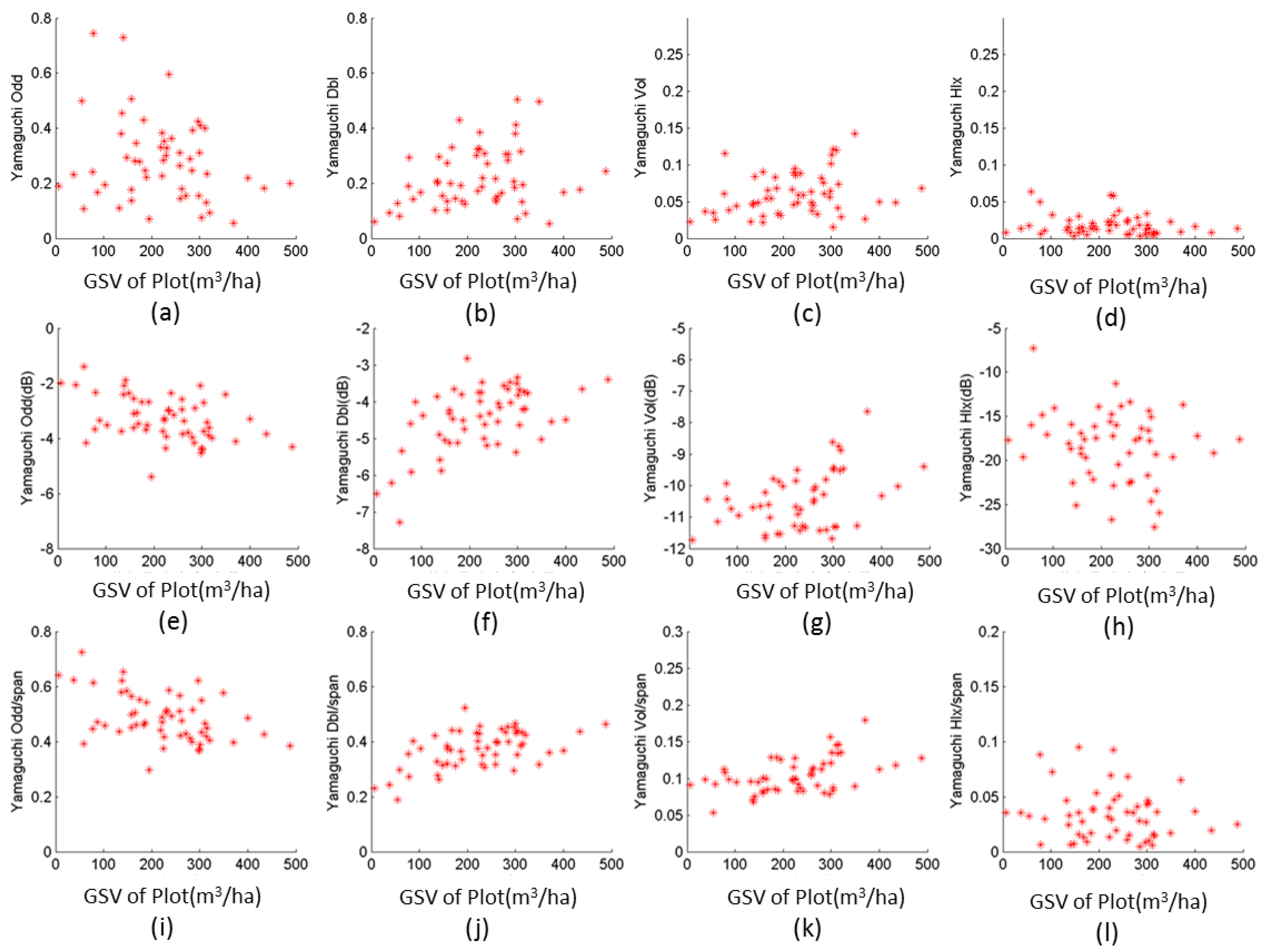
4.1. Polarimetric Characteristics

The polarimetric characteristics derived by the Yamaguchi decomposition were employed to interpret the interaction between forest GSV and the independent variables at the plot level (Figure 4). The Pearson correlation coefficient ($\gamma$) was adopted to select the characteristics for the GSV estimation based on a statistical test of correlation: Whether or not the correlation coefficients statistically were significantly different from zero at the significance level of 0.01. To match the size of the measured plots, the power value of scatterings in each plot was obtained by a window spatial averaging. Since the power of helix scattering (−30 dB to 10 dB) was too low (Figure 4d) compared with other scatterings (Figure 4a–c), it was not considered in the subsequent analysis. Moreover, the power of volume scattering (less than −8 dB) (Figure 4c) was also lower than those of the surface scattering (−5 dB to −2 dB) (Figure 4a) and double-bounce scattering (−7 dB to −3 dB) (Figure 4b). Before the transformation, the power of double-bounce (Figure 4b) and volume scattering (Figure 4c) increased slightly with the increasing GSV. After the logarithm and ratio transformations, the positive correlation became stronger (Figure 4f,g,j,k). All the correlation coefficients of the original scattering components were significantly smaller than the critical value of 0.345 at the risk level of 0.01 and these components were thus omitted in the subsequent analysis.

As shown in

Table 3. Pearson’s correlation coefficients R between the forest plot GSV and the polarimetric characteristics (Odd, Dbl and Vol indicate the surface scattering, double-bounce scattering and volume scattering, respectively; dB and Ratio indicate the polarimetric characteristics after the logarithm and ratio transformations).

Variables	Data Acquired on 30 June		Data Acquired on 25 August
	R	P-Value	R	P-Value
Odd (dB)	−0.56	0.000	−0.48	0.000
Dbl (dB)	0.70	0.000	0.53	0.000
Vol (dB)	0.44	0.002	0.21	0.154
Odd (Ratio)	−0.57	0.000	−0.42	0.000
Dbl (Ratio)	0.69	0.000	0.40	0.000
Vol (Ratio)	0.45	0.001	0.25	0.074
Dbl/Odd	−0.57	0.000	−0.48	0.001
Vol/Odd	−0.63	0.000	−0.53	0.000
Dbl*Vol	−0.71	0.000	−0.48	0.000
Dbl*Vol/Odd	0.62	0.000	0.50	0.000

, after the logarithm and ratio transformation, the Pearson’s correlation coefficients were greatly improved and become statistically different from zero, with the maximum of 0.70 achieved by the logarithm transformation of double-bounce scattering. Compared with the original polarimetric characteristics, the combined or fused characteristics also significantly increased the correlation coefficients with the forest plot GSV. After the transformations, the single and fused polarimetric characteristics were significantly correlated with the forest GSV and considered as potential independent variables to estimate the forest GSV.

4.2. Saturation Level of Planted Forest

Before the estimation, the plots in the shadow regions were discarded. The values of three unknown parameters were obtained by solving the base empirical model using the non-linear algorithm and the proposed initial values (

Table 4. Two unknown parameters and saturation level k estimated using different variables (Odd, Dbl and Vol: Surface scattering, double-bounce and volume scattering, respectively).

	Image of 30 June 2016			Image of 25 August 2016
Variable	βs	βn	k	βs	βn	k
Odd(dB)	−5.15	−1.80	349.84	−3.53	−2.16	121.74
Dbl(dB)	−3.01	−6.88	188.13	−4.24	−6.37	62.38
Odd(Ratio)	0.31	0.67	268.95	0.45	0.63	113.69
Dbl(Ratio)	0.52	0.20	260.88	0.39	0.23	82.84
Dbl/Odd	2.01	5.95	179.22	2.60	4.63	193.71
Vol/Odd	0.64	3.66	140.05	1.17	2.59	89.80
Dbl*Vol	26.18	78.20	206.42	41.50	69.07	101.79
Dbl*Vol/Odd	−5.93	−41.30	141.05	−10.07	−28.83	130.81

). For the image acquired on 30 June 2016, the estimated saturation values ranged from 140.05 m³/ha to 349.84 m³/ha, and the greatest value was obtained by the power of surface scattering. Moreover, the saturation values varied with the polarimetric characteristics. The saturation value obtained using the power of the double-bounce scattering after the ratio transformation, 260.88 m³/ha, was slightly larger than that obtained using the double-bounce scattering after the logarithm transformation, 188.13 m³/ha. Additionally, the saturation values derived from the image acquired on 25 August 2016 were much smaller than those derived from the images acquired on 30 June 2016. Some of the estimated saturation values were smaller than 100 m³/ha.

The saturation values derived from the fused characteristics ranged from 140.05 m³/ha to 206.42 m³/ha for the image acquired on 30 June and from 89.80 m³/ha to 193.71 m³/ha for the image acquired on 25 August, which were slightly smaller than those by single variables (Table 4). As shown in Figure 5, the power of the surface scattering (Figure 5a,c) and the double-bounce scattering (Figure 5b,d) had the highest saturation level for the image dated on 30 June. On the contrary, it was obvious that the ranges of the saturation levels obtained by the fused variables were more stable (Figure 5e–h).

4.3. Forest GSV Estimated by the Univariate Method

With the estimated parameters, the GSV values of the planted forests were retrieved by the univariate models (

Table 5. The GSV estimation accuracy of the selected variables (Note: * and ** indicate the percentages of the plots with errors exceeding the threshold are larger than 10% and 20%, respectively).

Variable	Image of 30 June 2016				Image of 25 August 2016
	R2	RMSE (m3/ha)	RRMSE (%)	Notes	R2	RMSE (m3/ha)	RRMSE (%)	Notes
Odd (dB)	0.59	81.40	40.36	*	0.57	90.37	46.20	*
Dbl (dB)	0.64	69.19	33.94		0.51	80.03	39.17	*
Odd (Ratio)	0.57	78.30	38.27	*	0.24	68.67	36.89	**
Dbl (Ratio)	0.66	69.09	35.07		0.27	81.73	40.32	**
Dbl/Odd	0.62	75.62	31.13	*	0.39	125.70	56.60	**
Vol/Odd	0.53	71.13	33.70	*	0.62	78.35	38.61	*
Dbl*Vol	0.66	71.65	31.80	*	0.47	76.27	37.30	**
Dbl*Vol/Odd	0.59	71.04	35.14		0.52	74.06	41.67	*

). The leave-one-out cross-validation (LOOCV) was utilized for the accuracy assessment [60] based on the root mean square error (RMSE) and the coefficient of determination ($R^2$) between the estimated and observed GSV values. The relative RMSE (RRMSE = RMSE × 100/sample mean) was also employed. We used 120 m³/ha as a deviation threshold value between the measured and estimated GSV values and counted the number of the plots with the errors exceeding the threshold. The reason for using the 120 m³/ha as the deviation threshold value was because this value was 50% of the sample mean 240 m³/ha and when the error of an estimate was larger than 50% of the sample mean, the estimate could be considered to be highly problematic.

In Table 5, scattering mechanisms had great impacts on the forest GSV estimation accuracy. As mentioned previously, the power of volume scattering was insufficient to describe the relationship between the forest GSV and the polarimetric characteristics. The power of surface scattering could successfully estimate the saturation value but more than one third of the selected plots were excluded, since their errors exceeded the given threshold. The minimum RMSE (69.19 m³/ha) and RRMSE (33.94%) between the estimated and measured GSV were obtained by the logarithm transformation of Dbl. The Dbl was thus more sensitive to the change of the forest GSV than the others.

The fused polarimetric characteristics were also used to estimate the forest GSV (Table 5). For the image acquired on 30 June, the fused characteristics led to the determination coefficients (R²) ranging from 0.53 to 0.66 and the maximum coefficient (0.66) was obtained by Dbl × Vol. The RMSE ranged from 71.04 m³/ha to 75.62 m³/ha. Therefore, using the fused characteristics could improve the accuracy of forest GSV estimation. The correlation coefficients and saturation levels indicated that it was very hard to accurately estimate forest GSV using the single variables from the image acquired on 25 August.

Figure 6 compared the measured and estimated GSV values by the univariate method. The estimated GSV values were highly affected by the saturation value. The power of Dbl with high saturation levels (Figure 6a,b) had fewer plots with errors exceeding the threshold than that with low saturation levels (Figure 6c–f). The selected polarimetric characteristics became insensitive to the change of forest GSV if the GSV values exceeded the saturation value (Figure 6e,f).

The independent variables with different saturation levels had different sensitivities to the forest GSV. The range of the forest GSV estimates depended largely on both the independent variables and the obtained saturation levels. The selected polarimetric characteristics with low saturation levels could not be used to generate high values of forest GSV. The base empirical model is a univariate approach, and in this approach, just one polarimetric characteristic was selected and others were discarded because of low saturation levels. In fact, the discarded polarimetric characteristics might also contain useful information and should be introduced into the multivariate method to estimate forest GSV.

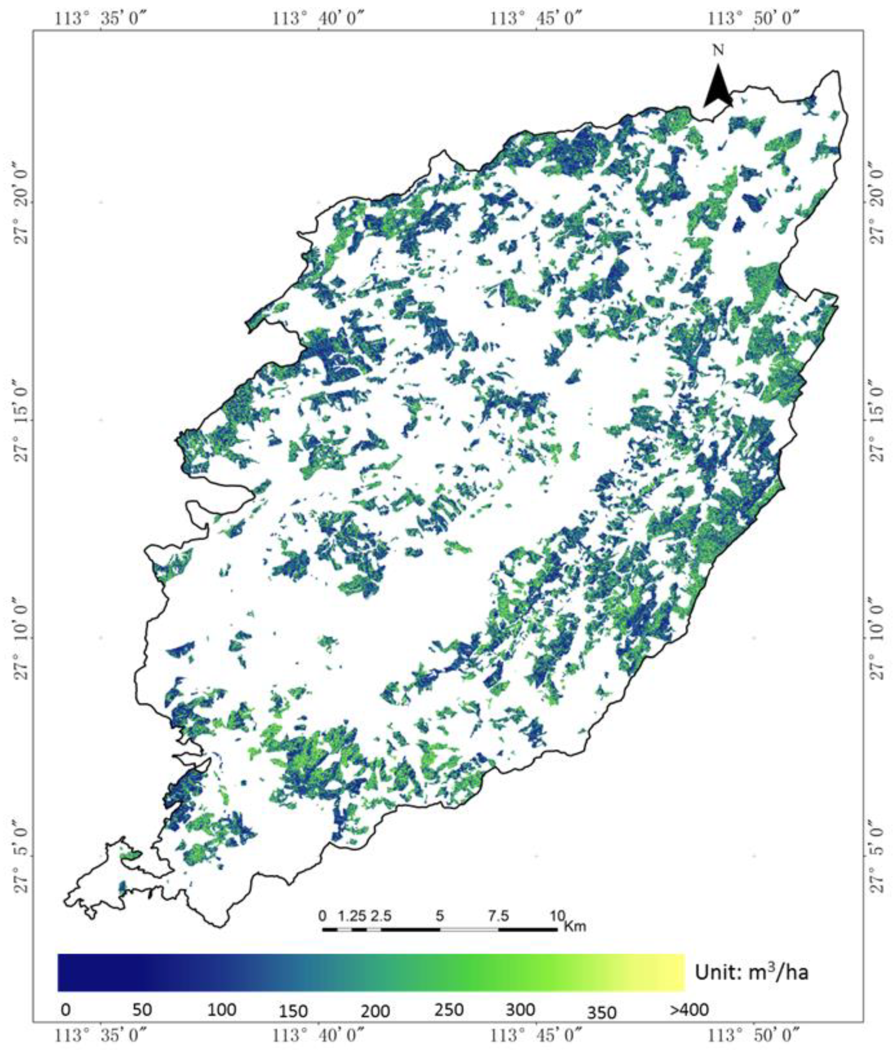
4.4. Forest GSV Estimated by the Saturation-Based Multivariate Method

To overcome the disadvantage of the base empirical model, we developed the saturation-based multivariate method, Equation (9), to improve the estimation of the forest GSV. According to the property of scattering mechanisms and the estimated saturation levels, three multivariate sets consisting of eight, six and four variables, respectively, were selected from each image to investigate the sensitivities of polarimetric characteristics. The set of the four variables consisted of four fused characteristics, including Dbl/Odd, Vol/Odd, Dbl ×Vol and Dbl × Vol/Odd. The set of the six variables consisted of the four fused variables, and the logarithm and ratio transformations of Dbl. The eight variables included the four fused variables, and the logarithm and ratio transformations of Odd and Dbl. The results of the saturation-based multivariate method are listed in

Table 6. The estimation accuracies of forest GSV using the saturation-based multivariate method.

Acquired Date	Number of Variables	Average of Errors (m3/ha)	Std of Errors (m3/ha)	RMSE (m3/ha)	RRMSE (%)
30 June 2016	8 Variables	67.42	31.01	74.06	35.09
	6 Variables	58.85	29.77	65.79	29.64
	4 Variables	61.89	34.21	70.53	30.88
25 August 2016	8 Variables	58.67	35.80	78.49	36.23
	6 Variables	66.72	35.01	80.15	38.84
	4 Variables	68.52	35.15	88.81	44.70

.

Compared with the univariate method, the saturation-based multivariate method led to higher estimation accuracy. The RRMSE ranged from 29.64% to 35.09% for the image acquired on June 30 and from 36.23% to 44.70% for the image acquired on 25 August. Moreover, the smallest RMSE and RRMSE values were 65.79 m³/ha and 29.64%, obtained by the set of the six variables that were involved in Equation (9). Additionally, the scatter graphs between the observed and estimated GSV values (Figure 6g,i) showed that compared with those from the univariate method, overall, the overestimations and underestimation were greatly reduced by the saturation-based multivariate method. Specially, for the plot that had the forest GSV values larger than the saturation points, the estimation accuracy was significantly improved by the saturation-based multivariate method. In Figure 7, the GSV of the Chinese fir plantations was mapped using the saturation-based multivariate method with the set of the six variables derived from the image dated 30 June 2016. The estimated GSV values varied from 50 m³/ha to 450 m³/ha.

5. Discussion

5.1. Polarimetric Characteristics Related to Tree Species

In this study, the measured GSV of Chinese fir plantations showed strong positive correlations with the power of double-bounce scattering, and strong negative correlations with the power of surface scattering (Table 3), but weak correlations with the power of volume scattering. Several factors may influence the correlations between the scattering mechanisms and forest GSV, and tree species might be the dominant factor. In the mixed forests of Siberia, the power of the volume scattering derived by the Yamaguchi decomposition showed high correlations with the measured GSV using L-band ALOS PALSAR data [20,21,29,31,36]. In the fast-growing forests in Indonesia, the surface scattering showed a negative correlation with the forest GSV (−0.70) and the volume scattering had a positive correlation with the forest GSV (0.45), but the double-bounce scattering was weakly correlated with the forest GSV [29]. In tropical forests, the power of volume scattering derived from the airborne L-band SAR data had positive correlations with the forest GSV [36]. The reasons for the different results might be mainly due to different tree species, thus different forest canopy structures. In Siberia, the percentage of broad-leaf species ranged from 29% to 44% [20,21,31], and in Indonesia and tropical forests [29,36], broad-leaf species were considered as dominated tree species and the power of volume scattering became strong by increasing the density of leaves. The strong correlations between the power of volume scattering and forest GSV were thus observed in the studies. In this study, however, the planted Chinese fir forests had narrow and short needles that led to many canopy gaps, thus the power of volume scattering could not account for the interaction between the forest canopy structures and the polarimetric characteristics. Moreover, tree trunks and big branches were the dominant scattering objects under the canopies, thus the double-bounce scattering was much stronger than that of volume scattering. This was especially true in the mature and over mature stands.

5.2. Saturation Level of Forest GSV

For a single SAR image, the saturation value is determined by two factors, including the estimation model and the polarimetric characteristics used. The empirical models have been widely employed to map GSV, in which the saturation level is estimated as a parameter. In this study, using the base empirical model with different independent variables, led to the different saturation values of GSV for the Chinese fir forests. The saturation values ranged from 140.05 m³/ha to 349.84 m³/ha (Table 4) and the greatest value was obtained using the power of surface scattering. The saturation values estimated by the double bounce scattering acquired on 25 August were about 63 m³/ha, seeming unreasonable. Some of variables, such as volume scattering, failed to result in the saturation values of the forest GSV, due to their low correlation to the plot GSV.

Theoretically, the power of surface scattering seems to be more sensitive to the forest GSV but the results of this study showed different (Table 5). The major reason was the existence of many forest canopy gaps in the Chinese fir plantations, which made the power of surface scattering related to the ground under the forest canopies, and led to a weak capacity to capture the forest GSV. This was especially true in the mature forests. The double bounce scattering was directly related to tree trunks and big branches and was very sensitive to the changes of the forest GSV. Furthermore, the fused variables formed by multiplication or division of the polarimetric characteristics greatly reduced the overestimations and underestimations of the saturation values, thus greatly improved the estimation accuracy. The saturation levels from the models that used the fused polarimetric characteristics were more reasonable and stable.

The great differences of the saturation levels derived from two SAR images were observed in Table 4. This might be mainly due to different weather conditions when the images were acquired. When the first image dated 30 June was collected, the weather was cloudy and the clouds had less impact on the quality of the image. However, there were showers on 25 August, on which date the second image was acquired. Moreover, it had been rainy for three days before 25 August. The showers and moisture might have great impact on the quality of the second image, and thus resulted in a low Pearson’s correlation between the GSV and the polarimetric characteristics from the image acquired from 25 August. The saturation levels derived from the SAR image acquired on 25 August were obviously lower than those from the first image acquired on 30 June.

5.3. Estimated GSV of Chinese Fir Plantation

The base empirical model has been frequently applied to express the interaction between polarimetric characteristics and forest GSV [36,37,38,39,40]. When one independent variable was employed, the estimated GSV values were closely related to the saturation level obtained (Table 4). For the power of Dbl after the ratio transformation, the RRMSE of the estimated GSV values with a large saturation value (260.88 m³/ha) was much smaller than that with a small saturation value (82.84 m³/ha). The error between the measured and estimated GSV values was significantly large when the measured GSV was larger than the saturation value (Figure 6a,e,f). The accuracy of the estimated GSV values also depended on the sensitivity of the independent variables. The different polarimetric characteristics led to different saturation values of the forest GSV, and thus different estimation accuracies. Overall, the fused characteristics resulted in more reasonable saturation values, thus much higher estimation accuracies of the forest GSV (Table 5).

In this study, the univariate method led to the smallest RRMSEs of 31.13% and 36.89%, for the images acquired on 30 June and 25 August 2016, respectively. Using the saturation-based multivariate method, the corresponding smallest RRMSE values were 29.64% and 36.23%, for the images acquired on 30 June and 25 August 2016, respectively. Compared with the univariate method, the saturation-based multivariate method obviously decreased the errors of the estimated GSV values. Additionally, the accuracy of the estimated GSV values was not related to the number of the used variables. The most accurate results were obtained by the saturation-based multivariate method with six variables from the image acquired on 30 June.

6. Conclusions

In this study, the powers of scatterings derived by the Yamaguchi decomposition were used to estimate the saturation values and forest GSV of Chinese fir plantations located in the hilly area of southern China using two quad-polarimetric PALSAR-2 images. The saturation value of the forest GSV was estimated by the univariate empirical model based on the single and fused characteristics. A novel and saturation-based multivariate method was then proposed by selecting and integrating the results from the univariate empirical models to improve the estimation accuracy of mapping the forest GSV in the study area. It was newly found that all the original polarimetric characteristics had weak correlations with the forest GSV and the power of double-bounce scattering was more sensitive to the forest GSV than the other polarimetric characteristics. Overall, the logarithm and ratio transformations of the scatterings greatly improved the correlations with the forest GSV, and further improvement of the correlation was achieved by the fused polarimetric characteristics. Moreover, the greatest saturation value was obtained using the logarithm transformation of surface scattering, but among the transformations of the polarimetric characteristics, the logarithm transformation of double-bounce scattering resulted in the smallest RRMSEs of the GSV estimates. Compared with the single transformations, the fused variables led to more reasonable saturation values and obviously reduced the values of RRMSE. More importantly, compared with the univariate method, the saturation-based multivariate method led to more accurate estimates of the forest GSV by reducing the overestimations and underestimations, with the smallest value (29.64%) of RRMSE achieved using the set of six variables. In addition, the SAR image dated 30 June provided better performance than the image dated 25 August. In summary, the novel saturation-based multivariate method provided the potential to improve the estimation accuracy of the Chinese fir forest GSV.

References

1. Di Cosmo, L.; Gasparini, P.; Tabacchi, G. A national-scale, stand-level model to predict total above-ground tree biomass from growing stock volume. For. Ecol. Manag. 2016, 361, 269–276. [Google Scholar] [CrossRef]
2. Krejza, J.; Světlík, J.; Bedná, P. Allometric relationship and biomass expansion factors (BEFs) for above- and below-ground biomass prediction and stem volume estimation for ash (Fraxinus excelsior L.) and oak (Quercus robur L.). Trees 2017, 31, 1303–1316. [Google Scholar] [CrossRef]
3. Wijaya, A.; Kusnadi, S.; Gloaguen, R.; Heilmeier, H. Improved strategy for estimating stem volume and forest biomass using moderate resolution remote sensing data and GIS. J. For. Res.-JPN 2010, 21, 1–12. [Google Scholar] [CrossRef]
4. Mathieu, R.; Naidoo, L.; Cho, M.A.; Leblon, B.; Main, R. Toward structural assessment of semi-arid African savannahs and woodlands: The potential of multitemporal polarimetric RADARSAT-2 fine beam images. Remote Sens. Environ. 2013, 138, 215–231. [Google Scholar] [CrossRef]
5. Silva, C.A.; Klauberg, C.; Hudak, A.T.; Vierling, L.A.; Liesenberg, V.; Carvalho, S.P.C.E.; Rodriguez, L.C.E. A principal component approach for predicting the stem volume in Eucalyptus plantations in Brazil using airborne LiDAR data. Forestry 2016, 89, 422–433. [Google Scholar] [CrossRef]
6. Abdullahi, S.; Kugler, F.; Pretzsch, H. Prediction of stem volume in complex temperate forest stands using TanDEM-X SAR data. Remote Sens. Environ. 2016, 174, 197–211. [Google Scholar] [CrossRef]
7. Chowdhury, T.A.; Thiel, C.; Schmullius, C.; Stelmaszczukgórska, M. Polarimetric Parameters for Growing Stock Volume Estimation Using ALOS PALSAR L-Band Data over Siberian Forests. Remote Sens. 2013, 5, 5725–5756. [Google Scholar] [CrossRef] [Green Version]
8. Iizuka, K.; Tateishi, R. Simple Relationship Analysis between L-Band Backscattering Intensity and the Stand Characteristics of Sugi and Hinoki Trees. Adv. Remote Sens. 2014, 3, 219–234. [Google Scholar] [CrossRef]
9. Joshi, N.; Mitchard, E.T.A.; Brolly, M.; Schumacher, J.; Fernándezlanda, A.; Johannsen, V.K.; Marchamalo, M.; Fensholt, R. Understanding ‘saturation’ of radar signals over forests. Sci. Rep. 2017, 7, 3505. [Google Scholar] [CrossRef]
10. Antropov, O.; Rauste, Y.; Ahola, H.; Hame, T. Stand-Level Stem Volume of Boreal Forests from Spaceborne SAR Imagery at L-Band. IEEE J. Sel. Top. Appl. Earth Obs. Remote Sens. 2013, 6, 35–44. [Google Scholar] [CrossRef]
11. Thiel, C.; Schmullius, C. The potential of ALOS PALSAR backscatter and InSAR coherence for forest growing stock volume estimation in Central Siberia. Remote Sens. Environ. 2016, 173, 258–273. [Google Scholar] [CrossRef]
12. Stelmaszczuk-Górska, M.; Rodriguez-Veiga, P.; Ackermann, N.; Thiel, C.; Balzter, H.; Schmullius, C. Non-Parametric Retrieval of Aboveground Biomass in Siberian Boreal Forests with ALOS PALSAR Interferometric Coherence and Backscatter Intensity. J. Imaging 2016, 2, 1. [Google Scholar] [CrossRef]
13. Santoro, M.; Schmullius, C.; Pathe, C.; Schwilk, J. Pan-boreal mapping of forest growing stock volume using hyper-temporal Envisat ASAR ScanSAR backscatter data. In Proceedings of the 2012 IEEE International Geoscience and Remote Sensing Symposium, Munich, Germany, 22–27 July 2012. [Google Scholar]
14. Santoro, M.; Eriksson, L.; Askne, J.; Schmullius, C. Assessment of stand-wise stem volume retrieval in boreal forest from JERS-1 L-band SAR backscatter. Int. J. Remote Sens. 2006, 27, 3425–3454. [Google Scholar] [CrossRef]
15. Fransson, J.E.S. Estimation of stem volume in boreal forests using ERS-1 C-and JERS-1 L-band SAR data. Int. J. Remote Sens. 1999, 20, 123–137. [Google Scholar] [CrossRef]
16. Santoro, M.; Beer, C.; Cartus, O.; Schmullius, C.; Shvidenko, A.; Mccallum, I.; Wegmüller, U.; Wiesmann, A. Retrieval of growing stock volume in boreal forest using hyper-temporal series of Envisat ASAR ScanSAR backscatter measurements. Remote Sens. Environ. 2011, 115, 490–507. [Google Scholar] [CrossRef]
17. Santoro, M.; Cartus, O.; Fransson, J.E.S.; Shvidenko, A.; Mccallum, I.; Hall, R.J.; Beaudoin, A.; Beer, C.; Schmullius, C. Estimates of Forest Growing Stock Volume for Sweden, Central Siberia, and Québec Using Envisat Advanced Synthetic Aperture Radar Backscatter Data. Remote Sens. 2013, 5, 4503–4532. [Google Scholar] [CrossRef]
18. Santoro, M.; Askne, J.; Smith, G.; Fransson, J.E.S. Stem volume retrieval in boreal forests from ERS-1/2 interferometry. Remote Sens. Environ. 2002, 81, 19–35. [Google Scholar] [CrossRef]
19. Santoro, M.; Shvidenko, A.; McCallum, I.; Askne, J.; Schmullius, C. Properties of ERS-1/2 coherence in the Siberian boreal forest and implications for stem volume retrieval. Remote Sens. Environ. 2007, 106, 154–172. [Google Scholar] [CrossRef]
20. Chowdhury, T.A.; Thiel, C.; Schmullius, C. Growing stock volume estimation from L-band ALOS PALSAR polarimetric coherence in Siberian forest. Remote Sens. Environ. 2014, 155, 129–144. [Google Scholar] [CrossRef]
21. Thiel, C.; Schmullius, C. Impact of Tree Species on Magnitude of PALSAR Interferometric Coherence over Siberian Forest at Frozen and Unfrozen Conditions. Remote Sens. 2014, 6, 1124–1136. [Google Scholar] [CrossRef] [Green Version]
22. Thiel, C.; Schmullius, C. Investigating ALOS PALSAR interferometric coherence in central Siberia at unfrozen and frozen conditions: Implications for forest growing stock volume estimation. Can. J. Remote Sens. 2013, 39, 232–250. [Google Scholar] [CrossRef]
23. Karila, K.; Vastaranta, M.; Karjalainen, M.; Kaasalainen, S. Tandem-X interferometry in the prediction of forest inventory attributes in managed boreal forests. Remote Sens. Environ. 2015, 159, 259–268. [Google Scholar] [CrossRef]
24. Cloude, S.R.; Zebker, H. Polarisation: Applications in Remote Sensing. Phys. Today 2010, 63, 53–54. [Google Scholar]
25. Lee, J.S.; Pottier, E. Polarimetric Radar Imaging: Basics to Applications, 2nd ed.; CRC Press: Boca Raton, FL, USA, 2016. [Google Scholar]
26. Freeman, A.; Durden, S.L. A three-component scattering model for polarimetric SAR data. IEEE Trans. Geosci. Remote Sens. 1998, 36, 963–973. [Google Scholar] [CrossRef] [Green Version]
27. Freeman, A. Fitting a two-component scattering model to polarimetric SAR data from forests. IEEE Trans. Geosci. Remote Sens. 2007, 45, 2583–2592. [Google Scholar] [CrossRef]
28. Yamaguchi, Y.; Moriyama, T.; Ishido, M.; Yamada, H. Four-component scattering model for polarimetric SAR image decomposition. IEEE Trans. Geosci. Remote Sens. 2005, 43, 1699–1706. [Google Scholar] [CrossRef]
29. Kobayashi, S.; Omura, Y.; Sangangoie, K.; Widyorini, R.; Kawai, S.; Supriadi, B.; Yamaguchi, Y. Characteristics of Decomposition Powers of L-Band Multi-Polarimetric SAR in Assessing Tree Growth of Industrial Plantation Forests in the Tropics. Remote Sens. 2012, 4, 3058–3077. [Google Scholar] [CrossRef] [Green Version]
30. Antropov, O.; Rauste, Y.; Hame, T. Volume scattering modeling in PolSAR decompositions: Study of ALOS PALSAR data over boreal forest. IEEE Trans. Geosci. Remote Sens. 2011, 49, 3838–3848. [Google Scholar] [CrossRef]
31. Huang, L.Y.; Yan, Q.L.; Gao, T.; Zhu, J.J. Estimation on stock volume of plantation forests using ALOS PALSAR images: A case study of Larix principis-rupprechtii plantations in Saihanba Forest Farm. Chin. J. Ecol. 2015, 34, 2401–2409. [Google Scholar]
32. Kobayashi, S.; Omura, Y.; Sanga-Ngoie, K.; Yamaguchi, Y.; Widyorini, R.; Fujita, M.S.; Supriadi, B.; Kawai, S. Yearly Variation of Acacia Plantation Forests Obtained by Polarimetric Analysis of ALOS PALSAR Data. IEEE J. Sel. Top. Appl. Earth Obs. Remote Sens. 2016, 8, 5294–5304. [Google Scholar] [CrossRef]
33. Yuan, J.; Li, Y.M.; Liu, C.L.; Zha, X.F. Leave-One-Out Cross-Validation Based Model Selection for Manifold Regularization; Springer: Berlin/Heidelberg, Germany, 2010. [Google Scholar]
34. Askne, J.; Santoro, M.; Smith, G.; Fransson, J.E.S. Multitemporal repeat-pass SAR interferometry of boreal forests. IEEE Trans. Geosci. Remote Sens. 2005, 43, 1219–1228. [Google Scholar] [CrossRef]
35. Pulliainen, J.; Engdahl, M.; Hallikainen, M. Feasibility of multi-temporal interferometric SAR data for stand-level estimation of boreal forest stem volume. Remote Sens. Environ. 2003, 85, 397–409. [Google Scholar] [CrossRef]
36. Gonçalves, F.G.; Santos, J.R.; Treuhaft, R.N. Stem volume of tropical forests from polarimetric radar. Int. J. Remote Sens. 2011, 32, 503–522. [Google Scholar] [CrossRef]
37. Olesk, A.; Praks, J.; Antropov, O.; Zalite, K.; Arumäe, T.; Voormansik, K. Interferometric SAR Coherence Models for Characterization of Hemiboreal Forests Using TanDEM-X Data. Remote Sens. 2016, 8, 700. [Google Scholar] [CrossRef]
38. Zhang, H.; Zhu, J.; Wang, C.; Lin, H.; Long, J.; Zhao, L.; Fu, H.; Liu, Z. Forest Growing Stock Volume Estimation in Subtropical Mountain Areas Using PALSAR-2 L-Band PolSAR Data. Forests 2019, 10, 276. [Google Scholar] [CrossRef]
39. Wang, C.; Wang, L.; Fu, H.; Xie, Q.; Zhu, J.; Wang, C.; Wang, L.; Fu, H.; Xie, Q.; Zhu, J. The Impact of Forest Density on Forest Height Inversion Modeling from Polarimetric InSAR Data. Remote Sens.-Basel 2016, 8, 291. [Google Scholar] [CrossRef]
40. Wagner, W.; Luckman, A.; Vietmeier, J.; Tansey, K.; Balzter, H.; Schmullius, C.; Davidson, M.; Gaveau, D.; Gluck, M.; Toan, T.L. Large-scale mapping of boreal forest in SIBERIA using ERS tandem coherence and JERS backscatter data. Remote Sens. Environ. 2003, 85, 125–144. [Google Scholar] [CrossRef]
41. Wang, Z.M.; Zhang, W.Q.; Yue, C.R.; Liu, Q. Estimation of Forest Growing Stock Based on TerraSAR-X and ALOS PALSAR Data:a Case Study in Mengla County of Yunnan Province. J. Zhejiang For. Sci. Technol. 2018, 38, 38–42. [Google Scholar]
42. Yang, M.; Wang, Y.; Zhang, X. Study on the model for estimating forest volume of Chinese fir based on bi-source remote sensing data. J. Nanjing For. Univ. 2016, 40, 107–114. [Google Scholar]
43. Dong, G.; Jian, Y.; Peng, Y.; Chao, W.; Hong, Z. Forest characteristic detection with Pol-SAR. J. Tsinghua Univ. 2003, 43, 953–956. [Google Scholar]
44. Xi, F. Density, storage and distribution of carbon in Chinese fir plantation at fast growing stage. Sci. Silv. Sin. 2002, 38, 14–19. [Google Scholar]
45. Zhang, X.; Zhang, J.; Duan, A. Compatibility of Stand Volume Model for Chinese Fir Based on Tree-Level and Stand-Level. Sci. Silv. Sin. 2014, 50, 82–87. [Google Scholar]
46. Zheng, D.; Hu, G.; Chen, P.; Gong, Z. The Selection and Error Analysis of the Angle Gauge Constant in the Chinese-fir Plantation at Different Ages. For. Resour. Manag. 2006, 2, 74–78. [Google Scholar]
47. Quegan, S.; Dutra, L.V. SAR Calibration and Principal Component Analysis. In Proceedings of the Third Airborne Synthetic Aperture Radar (AIRSAR) Workshop, Pasadena, CA, USA, 1 August 1991. [Google Scholar]
48. Freeman, A. Calibration of linearly polarized polarimetric SAR data subject to Faraday rotation. IEEE Trans. Geosci. Remote Sens. 2004, 42, 1617–1624. [Google Scholar] [CrossRef]
49. Chen, J.; Quegan, S. Calibration of Spaceborne CTLR Compact Polarimetric Low-Frequency SAR Using Mixed Radar Calibrators. IEEE Trans. Geosci. Remote Sens. 2011, 49, 2712–2723. [Google Scholar] [CrossRef]
50. Quegan, S.; Lomas, M. The interaction between calibration and Faraday rotation estimates from SAR. In Proceedings of the EUSAR European Conference on Synthetic Aperture Radar, Berlin, Germany, 3–5 June 2014. [Google Scholar]
51. Mohanty, S.; Singh, G.; Yamaguchi, Y. Faraday rotation correction and total electron content estimation using ALOS-2/PALSAR-2 full polarimetric SAR data. In Proceedings of the 2016 IEEE International Geoscience and Remote Sensing Symposium (IGARSS), Beijing, China, 10–15 July 2016. [Google Scholar]
52. Kimura, H.; Mizuno, T.; Papathanassiou, K.P.; Hajnsek, I. Improvement of polarimetric SAR calibration based on the Quegan algorithm. In Proceedings of the IEEE International Geoscience & Remote Sensing Symposium, Anchorage, AK, USA, 20–24 September 2004. [Google Scholar]
53. Lee, J.S.; Schuler, D.L.; Ainsworth, T.L. Polarimetric SAR data compensation for terrain azimuth slope variation. IEEE Trans. Geosci. Remote Sens. 2000, 38, 2153–2163. [Google Scholar]
54. Schuler, D.L.; Lee, J.S.; Grandi, G.D. Measurement of topography using polarimetric SAR images. IEEE Trans. Geosci. Remote Sens. 1996, 34, 1266–1277. [Google Scholar] [CrossRef]
55. Lee, J.S.; Schuler, D.L.; Ainsworth, T.L.; Krogager, E.; Kasilingam, D.; Boerner, W.M. On the estimation of radar polarization orientation shifts induced by terrain slopes. IEEE Trans. Geosci. Remote Sens. 2002, 40, 30–41. [Google Scholar]
56. Yi, X.; Hoffmeyer, P.D.; Narayanan, R.M.; Curtis, J.O. Signal processing aspects of polarimetric random noise radar data for shallow subsurface imaging. In Proceedings of the International Geoscience & Remote Sensing Symposium, Lincoln, NE, USA, 31–31 May 1996. [Google Scholar]
57. Cloude, S.R.; Pottier, E. A review of target decomposition theorems in radar polarimetry. IEEE Trans. Geosci. Remote Sens. 1996, 34, 498–518. [Google Scholar] [CrossRef]
58. Cameron, W.L.; Leung, L.K. Feature motivated polarization scattering matrix decomposition. In Proceedings of the IEEE International Radar Conference, Arlington, VA, USA, 7–10 May 1990. [Google Scholar]
59. Xu, F.; Jin, Y.Q. Deorientation theory of polarimetric scattering targets and application to terrain surface classification. IEEE Trans. Geosci. Remote Sens. 2005, 43, 2351–2364. [Google Scholar]
60. Loew, A.; Mauser, W. Generation of geometrically and radiometrically terrain corrected SAR image products. Remote Sens. Environ. 2007, 106, 337–349. [Google Scholar] [CrossRef]
61. Logan, T.A.; Nicoll, J.; Laurencelle, J.; Hogenson, K.; Gens, R.; Buechler, B.; Barton, B.; Shreve, W.; Stern, T.; Drew, L. Radiometrically Terrain Corrected ALOS PALSAR Data Available from the Alaska Satellite Facility. In Proceedings of the AGU Fall Meeting, San Francisco, CA, USA, 15–19 December 2014. [Google Scholar]
Figure 1. (a) Location of the study area and (b) the distribution of tree species in the study area.
Remotesensing 11 01872 g001
Figure 2. (a) Distribution of the selected plots; and (b) the photos of ground measured plots with different age groups.
Remotesensing 11 01872 g002
Figure 3. (a) The ALOS PALSAR-2 Pauli RGB composite image acquired on 30 June, 2016 and (b) digital elevation model (DEM) of the study area with the black line outlining the study area.
Remotesensing 11 01872 g003
Figure 4. The relationships between the forest GSV and the components obtained by the Yamaguchi decomposition from the image of 30 June 2016: (ad) are the original scattering features; (eh) are the scattering features after the logarithm transformation; (il) are the scattering features after the ratio transformation. The Odd, Dbl, Vol and Hlx are the surface scattering, double-bounce scattering, volume scattering and helix scattering, respectively.
Remotesensing 11 01872 g004
Figure 5. Relationships between the forest GSV and polarimetric characteristics of the image acquired on 30 June 2016 by the semi-exponential model; (ad) are the results using the logarithm or ratio transformations of scatterings; (eh) are the results using the fused polarimetric characteristics.
Remotesensing 11 01872 g005
Figure 6. The scatter graphs between the observed and estimated GSV values of the plots using the image dated on 30 June 2016: (a,b) are the GSV estimated by the powers of Dbl after logarithm and ratio transformation, respectively; (cg) are the GSV estimated by the fused variables; (gi) are the GSV estimated from the saturation-based multivariate approach with eight variables, six variables and four variables, respectively.
Remotesensing 11 01872 g006
Figure 7. The GSV map of the planted Chinese fir forests in the study area estimated by the saturation-based multivariate method using the set of the six variables derived from the image dated on 30 June 2016.
Remotesensing 11 01872 g007