Airborne LIDAR-Derived Aboveground Biomass Estimates Using a Hierarchical Bayesian Approach

Abstract

Conventional ground survey data are very accurate, but expensive. Airborne lidar data can reduce the costs and effort required to conduct large-scale forest surveys. It is critical to improve biomass estimation and evaluate carbon stock when we use lidar data. Bayesian methods integrate prior information about unknown parameters, reduce the parameter estimation uncertainty, and improve model performance. This study focused on predicting the independent tree aboveground biomass (AGB) with a hierarchical Bayesian model using airborne LIDAR data and comparing the hierarchical Bayesian model with classical methods (nonlinear mixed effect model, NLME). Firstly, we chose the best diameter at breast height (DBH) model from several widely used models through a hierarchical Bayesian method. Secondly, we used the DBH predictions together with the tree height (LH) and canopy projection area (CPA) derived by airborne lidar as independent variables to develop the AGB model through a hierarchical Bayesian method with parameter priors from the NLME method. We then compared the hierarchical Bayesian method with the NLME method. The results showed that the two methods performed similarly when pooling the data, while for small sample sizes, the Bayesian method was much better than the classical method. The results of this study imply that the Bayesian method has the potential to improve the estimations of both DBH and AGB using LIDAR data, which reduces costs compared with conventional measurements.

1. Introduction

On the world’s land surface, forests cover about 4200 million hectares, and the carbon stock of forests accounts for about 45% of the world’s terrestrial carbon reserves [1]. Aboveground biomass is an important component of forest ecosystems and accounts for a large proportion of forest carbon stock; thus, quantifying forest aboveground biomass is important for forest managers [2].

Diameter at breast height (DBH) and aboveground biomass (AGB) are two important measurements of individual trees, widely used in yield estimations and forest growth [3]. Tree DBH is an easy measuring factor with high accuracy—all DBH data are measured. However, AGB is difficult to measure and has less accuracy than ground-observed DBH—only limited tree biomass can be measured in the sample [4]. Consequently, in the past few decades, many studies have proposed numerous equations to estimate aboveground biomass [5,6,7,8,9,10]. Developing an AGB model according to ground-based DBH has been widely applied in forest investigation and yield modeling. It is important to note that DBH measurement in large-scale forest inventory is still time-consuming and costly.

LIDAR is a range detection system, which obtains the forest point cloud by LIDAR sensors. The LIDAR system has been used to measure the forest vegetation structure and has been applied to measure forest variables since the mid-1980s [11]. These variables, including tree height, stem volume, crown projection area, diameter at breast height, and other variables, are significantly connected to the forest biomass [3,11,12]. Using these LIDAR variables, individual tree DBH and aboveground biomass can be estimated by developing DBH and AGB models, respectively [3,12,13]. With some studies also using LIDAR data to predict timber volume and discern age class, LIDAR data have been widely used in forestry over the past two decades. The application of LIDAR technology has reduced the cost of forest management and provided a good opportunity for large-scale forest inventory [11,12].

The Bayesian method is used to integrate prior information about unknown parameters with the sample information; then, the posterior information is obtained according to the Bayes formula and the method of unknown parameters is further inferred according to the posterior information. Many studies have already used the Bayesian method to develop DBH and AGB models and have compared the Bayesian model with the classical model [14,15,16,17]. Zapata-Cuartas et al. [14] presented a comparison of aboveground biomass estimation in different sample sizes using the Bayesian method and the classical method. They obtained a result that the bias in the classical method was always bigger than that in the Bayesian approach.

Although LIDAR technology and Bayesian methods are used separately in individual DBH and AGB modeling [6,13,14,15,17,18,19,20,21], few studies have combined the two methods to estimate DBH and aboveground biomass. Tenneson [22] presented a combination of the Bayesian method and LIDAR to model LIDAR-derived forest inventory, combining the advantages of both DBH and AGB prediction; they used Bayesian model averaging (BMA), while we are using the hierarchical Bayesian method [23,24]. In this study, we used the hierarchical Bayesian method to choose the best DBH and AGB model to predict DBH and aboveground biomass on the basis of LIDAR point cloud data, integrating the advantages of the Bayesian approach and LIDAR data to reduce costs compared with conventional measurements [13,14]. Further, compared with the classical prediction method, using the Bayesian method can improve the accuracy to a certain degree.

2. Materials and Methods

2.1. Study Area and Data

The study area from which data were taken is located at the Xishui forest farm of Su’nan Yuguzu Autonomous County, China (38°290–38°350N, 100°120–100°200E) and lies within the temperate alpine cold semi-humid and semi-arid zone. The altitude is in the 2550 to 3680 m range, with a mean value of 2993 m in this area. This area is occupied by mountainous forests and steppes, and one of the main functions of these forests is to protect the water resources in the Dayekou Basin of the Qilian Mountains. Grass and natural mature secondary pure forests dominate the sunny and shady slopes, respectively. The dominant tree species in the forest in this area is Picea crassifolia Kom.

We established a single permanent sample plot (PSP) of 100 m × 100 m along the hillside and divided it into sixteen subplots of 25 m × 25 m. DBH, tree height (H), crown base height, and crown diameters in two perpendicular directions of all standing trees were measured in each subplot. We used a differential global positioning system unit to measure the corners and centers of the PSP in each subplot, and a total station to measure the positions of individual trees.

Airborne LIDAR data were acquired using a Lite Mapper 5600 system on 23 June 2008. The mean flight speed was 230 km h⁻¹ and the mean flight height was 3699 m above sea level. The point elevation varied from 2725 to 3193 m, and the LIDAR point density was 4.34 points m⁻². We can obtain individual LIDAR tree heights and crown projection areas on the basis of the airborne LIDAR point cloud from a canopy height model (CHM), and the CHM was derived as the difference between the digital surface model (DSM) and the digital elevation model (DEM) of the study area. The digital surface model grid, which contained elevation information including all ground objects, was interpolated from raw LIDAR point cloud data by a maximum height interpolation method and by filling null cells. For obtaining the absolute vegetation heights, we must remove the influence of the terrain. Thus, we obtained the digital elevation model from the ground-classified LIDAR point cloud data using a progressive morphological filter and, in this study, with a grid cell size of 0.5 m [3]. We also eliminated the noise using a Gaussian smoothing filter to obtain a more accurate crown projection area [3]. We used the local maxima algorithm to find the individual tree crown tops, and used the region growing method to obtain the tree crown boundary, the crown projection area was calculated according to the determined tree crown boundary. The details of the algorithms can be found in Fu et al. [3]. A total of 402 individual P. crassifolia tree crowns in the 16 subplots nested in the PSP were delineated; the individual tree LIDAR crown projection area and field measurement data were matched by individual tree locations measured by total station—Fu et al. [3] has drawn a figure to explain this. The biomasses of each component (stem, branch, foliage, and fruit) of the 402 P. crassifolia trees were estimated using the empirical allometric models developed by Wang et al. [25] using the field-measured individual DBH and tree height H. The total tree AGB was obtained by summing the component biomass values. For more information about the study sites and data collection, please see Fu et al. [3].

2.2. Random Sampling

In order to compare the LIDAR AGB estimation by the Bayesian method and the classical method in different sample sizes, five samples (Samples 1–4) of different sizes were randomly selected from the population. The independent variables in the population, including LIDAR crown projection area (CPA), LIDAR tree height (LH), ground-measured DBH, and the ground-estimated AGB, were assessed. Sample 1 randomly sampled 10% of the population, and Samples 2–4 randomly sampled 25%, 50%, and 75% of the population, respectively. The statistics of sample sizes 1–4 are presented in (

Table 1. Summary statistics of different sample sizes (DBH, ground-measured diameter at breast height; LH, LIDAR tree height; CPA, crown projection area; AGB, ground-estimated aboveground biomass).

Sample Size	Factor	Maximum	Minimum	Mean	SD
10% (39)	DBH	36.40	2.50	21.26	7.84
	LH	9.79	1.96	6.81	2.17
	AGB	395.83	1.45	153.08	102.39
	CPA	11.06	2.94	7.42	2.20
25% (99)	DBH	40.50	8.20	23.38	7.77
	LH	10.10	2.21	6.80	1.88
	AGB	508.02	15.68	178.08	119.52
	CPA	12.80	3.56	7.32	1.97
50% (199)	DBH	54.50	2.50	22.73	7.41
	LH	11.29	1.96	6.96	1.85
	AGB	959.49	1.45	169.51	118.90
	CPA	13.50	2.94	7.48	2.03
75% (303)	DBH	54.50	2.50	23.09	7.78
	LH	11.30	1.96	6.92	1.89
	AGB	959.49	1.45	176.03	125.55
	CPA	13.50	2.94	7.41	2.06
100% (402)	DBH	81.10	2.50	23.40	8.30
	LH	11.20	1.90	6.90	1.90
	AGB	1142.50	1.45	181.30	134.10
	CPA	13.50	2.90	7.43	2.06

), and we also put the statistics of the full dataset into this table.

2.3. DBH and AGB Models

In this paper, four frequently used candidate model forms [3] and another three models [26,27,28] were used to develop LIDAR DBH estimation models by regarding the LIDAR-derived tree height and the crown projection area as the predictor variables. These models are listed as follows:

$$DBH={\beta }_1+{\beta }_{2}LH+{\beta }_{3}CPA+{\epsilon }_{DBH}(\mathrm{Linear})$$

I.1

$$DBH={\beta }_1[1-exp(-{\beta }_{2}LH-{\beta }_{3}CPA)]+{\epsilon }_{DBH}(\mathrm{Richards})$$

I.2

$$DBH={\beta }_1/[1+{\beta }_{2}exp(-{\beta }_{3}LH-{\beta }_{4}CPA)]+{\epsilon }_{DBH}(\mathrm{Logistic})$$

I.3

$$DBH={\beta }_{1}exp(-\beta {}_{2}LH-{\beta }_{3}CPA)+{\epsilon }_{DBH}(\mathrm{Exponential})$$

I.4

$$DBH=-{{\beta }_1}^{-1}\ln [1-({60}^{-1}(LH-1.3){)}^{1/{\beta }_2}]+{\epsilon }_{DBH}(\mathrm{Richards})$$

I.5

$$DBH=[-{{\beta }_1}^{-1}\ln {(1-{60}^{-1}(LH-1.3)]}^{1/{\beta }_2}+{\epsilon }_{DBH}([27])$$

I.6

$$DBH={\beta }_1{(LH-1.3)}^{{\beta }_2}exp({\beta }_{3}CPA)+{\epsilon }_{DBH}([28])$$

I.7

where β₁–β₄ are parameters of the models, LH is the LIDAR tree height, CPA is the LIDAR crown projection area, and ε_DBH is the error term.

On the basis of the best DBH model, five commonly used AGB model forms were applied to estimate the aboveground biomass. They are listed as follows:

$$AGB={\alpha }_{1}DB{H}^{{\alpha }_2}+{\epsilon }_{AGB}$$

II.1

$$AGB={\alpha }_{1}DB{H}^{{\alpha }_2}L{H}^{{\alpha }_3}+{\epsilon }_{AGB}$$

II.2

$$AGB={\alpha }_{1}DB{H}^{{\alpha }_2}CP{A}^{{\alpha }_3}+{\epsilon }_{AGB}$$

II.3

$$AGB={\alpha }_{1}L{H}^{{\alpha }_2}CP{A}^{{\alpha }_3}+{\epsilon }_{AGB}$$

II.4

$$AGB={\alpha }_{1}DB{H}^{{\alpha }_2}L{H}^{{\alpha }_3}CP{A}^{{\alpha }_4}+{\epsilon }_{AGB}$$

II.5

where α₁–α₃ are model parameters, DBH is the LIDAR estimated DBH, and ε_AGB is the error term.

2.4. Bayesian Method

Bayesian estimation is used to combine new evidence and prior distributions with the Bayesian theorem to get a new probability. Zhang et al. [16,29] presented the Bayesian rules in detail. Let y = (y₁, y₂, y₃, …) represent a vector of data and θ = (θ₁, θ₂, θ₃, …) be a vector of parameters to be estimated. Bayes’ expression is

$$p(y,\theta )=p(y|\theta )p(\theta )=p(\theta |y)p(y)$$

where p(θ) is the prior distribution for the parameters, which can be obtained by the classical method; and p(θ|y) is the posterior distribution of the Bayesian frameworks.

An important feature of the Bayesian method is that the parameter will be given a prior distribution before sampling. The choice of prior distribution is critical for the Bayesian method [25]. Non-informative priors with large or infinite variance that reflect prior “ignorance” are generally chosen [29,30,31]. Alternatively, if prior information is available from external knowledge (reported parameters from the literature), the information can be used to construct a prior distribution. Zhang et al. [32] used the parameter estimates of height growth models from classical method as the prior information for the Bayesian method, consistent with Zhang et al. [32]. Here, we used the parameters of NLME estimation as the prior distribution for the Bayesian estimation.

2.5. Model Evaluation

The best DBH and AGB model was chosen from the value of the deviance information criterion (DIC) [16], when pooling the data:

$$DIC=\overline{D}+N$$

where $\overline{D}=E_{\theta }\{-2\log [p(y|\theta )]\}$ represents the posterior mean of the deviance; and $N=\overline{D}+2\log [p(y|\overline{\theta })]$ is the effective number of parameters in the model and represents the complexity of the model. A smaller value of DIC for a model indicates a better fit to the data [31].

In addition, the stationarity test in Heidelberger–Welch Diagnostics [33,34] was regarded as a criterion to test if the model converged in our study. The stationary process is a random process in statistics, and its unconditional joint probability distribution does not change with time. Thus, the mean value and variance do not change with time either [35].

The determination coefficient (R²) and mean absolute deviation (MAD) were used to compare the Bayesian method with the classical method. Higher R² and smaller MAD values indicate a better model fit to the data. They are calculated by

$$R^2=\frac{\sum (y-\widehat{y}{)}^2}{\sum {(y-\overline{y})}^2},$$

$$MAD=\sum \left|y-\widehat{y}\right|/n,$$

where y is the observed AGB, $\widehat{y}$ is the LIDAR predicted DBH or AGB, $\overline{y}$ is the mean value of the observed AGB, and n is the number of samples.

This study developed several candidate DBH models and selected the best model. On the basis of the best DBH model, DBH predictions were introduced to the five candidate AGB models as one of the independent variables. Both the DBH and the AGB models were developed through the hierarchical Bayesian approach. In addition, five different random sample sizes were used for comparing the Bayesian method with the classical method.

Considering the random effects of plot, we added a random effect parameter to β₁ in DBH models and to α₁ in AGB models using hierarchical Bayesian and classical methods (nonlinear mixed effects model, NLME). The Bayesian and NLME models were constructed by using SAS procedures MCMC and MODEL, respectively [36]. For the Bayesian estimation, a burn-in period of 10,000 steps and 100,000 iterations was used to estimate parameters. The thinning parameter was set to 5 to reduce the correlation between neighboring iterations.

3. Results

3.1. Model Selection

In this study, deviance information criterion (DIC) statistics and the stationarity test were used to evaluate the Bayesian DBH and AGB models. As shown in

Table 2. Deviance information criterion (DIC) values and stationarity test of seven DBH candidate base models.

Model	DIC	Stationarity Test
I.1	2557.572	passed
I.2	2556.442	passed
I.3	2541.001	passed
I.4	2545.794	passed
I.5	-	failed
I.6	2580.574	passed
I.7	2547.292	passed

, all the DBH models other than model I.5 passed the stationarity test (Table 2). Model I.3 had the smallest DIC value, followed by I.4, I.7, I.2, I.1, and I.6. Thus, model I.3 was selected as the best model to predict DBH used as an independent variable for modeling AGB.

The parameter estimations of model I.3 for different sample sizes are listed in

Table 3. Parameter estimates and standard deviation errors/deviations (values in brackets) of the LIDAR DBH model for different sample sizes (NLME, nonlinear mixed effects model).

n	39	99	199	303	402
Bayesian
β1	49.34 (6.428)	99.62 (7.66)	99.58 (6.7)	99.44 (6.68)	111.3 (24.46)
β2	8.326 (1.326)	11.92 (1.408)	13.2 (1.223)	11.96 (1.213)	13.6 (2.79)
β3	−0.036 (0.045)	0.108 (0.04)	0.148 (0.025)	0.107 (0.03)	0.114 (0.024)
β4	0.297 (0.055)	0.068 (0.037)	0.043 (0.021)	0.072 (0.026)	0.066 (0.022)
NLME
β1	49.48 (9.75)	99.57 (64.35)	99.37 (50.25)	99.2 (47.63)	99.36 (42.52)
β2	8.246 (1.792)	11.75 (7.07)	13.04 (5.968)	11.83 (5.282)	12.29 (4.76)
β3	−0.036 (0.07)	0.108 (0.043)	0.146 (0.03)	0.109 (0.033)	0.118 (0.026)
β4	0.292 (0.092)	0.067 (0.042)	0.044 (0.026)	0.068 (0.03)	0.065 (0.025)

. In all sample sizes, the standard deviations of all the parameters estimated by the Bayesian method were smaller than those estimated by the classical method, meaning that the parameters estimated by the Bayesian method were more stable than those estimated by the classical method. Simultaneously, we can see from Table 3 that in Bayesian estimation, the range of parameters at sample size 39 was between −0.036 and 49.34, while it was between 0.066 and 111.3 at full data. The ranges of parameter estimates for small sample size were significantly narrower than those of the full data, which confirms that for a small sample size, the Bayesian method shows higher efficiency.

In terms of the fitting statistics, AGB models II.1, II.3, and II.4 passed the stationarity test (

Table 4. DIC values and stationarity test of the five AGB candidate models.

Model No.	DIC	Stationarity Test
II.1	4763.795	passed
II.2	-	failed
II.3	4754.906	passed
II.4	4777.023	passed
II.5	-	failed

), however, the other two models failed. Among the three models, II.1, II.3, and II.4, the DIC in II.3 (4754.906) was much smaller than those in the other two models. Therefore, model II.3 was selected as the best model to predict AGB. The parameter estimations of model II.3 are listed in

Table 5. Parameter estimates and standard deviation errors/deviations (values in brackets) of the LIDAR AGB model for different sample sizes.

n	39	99	199	303	402
Bayesian
α1	0.133 (0.0320)	0.027 (0.0097)	0.281 (0.0604)	0.281 (0.0604)	0.184 (0.0339)
α2	2.334 (0.3959)	3.385 (0.2338)	1.370 (0.1881)	1.37 (0.1881)	2.383 (0.1428)
α3	−0.246 (0.5815)	−1.332 (0.3225)	0.990 (0.2447)	0.990 (0.2447)	−0.346 (0.1825)
NLME
α1	0.014 (0.0461)	0.007 (0.0101)	0.167 (0.1068)	0.052 (0.0371)	0.096 (0.0506)
α2	3.522 (1.7199)	4.463 (0.8609)	1.670 (0.4611)	2.973 (0.3612)	2.781 (0.3620)
α3	−0.967 (1.254)	−2.019 (0.726)	0.765 (0.4559)	−0.617 (0.3463)	−0.652 (0.3438)

. The standard deviation of parameter estimations by Bayesian method in all sample sizes are smaller than classical method.

3.2. Comparing the Hierarchical Bayesian and NLME Methods

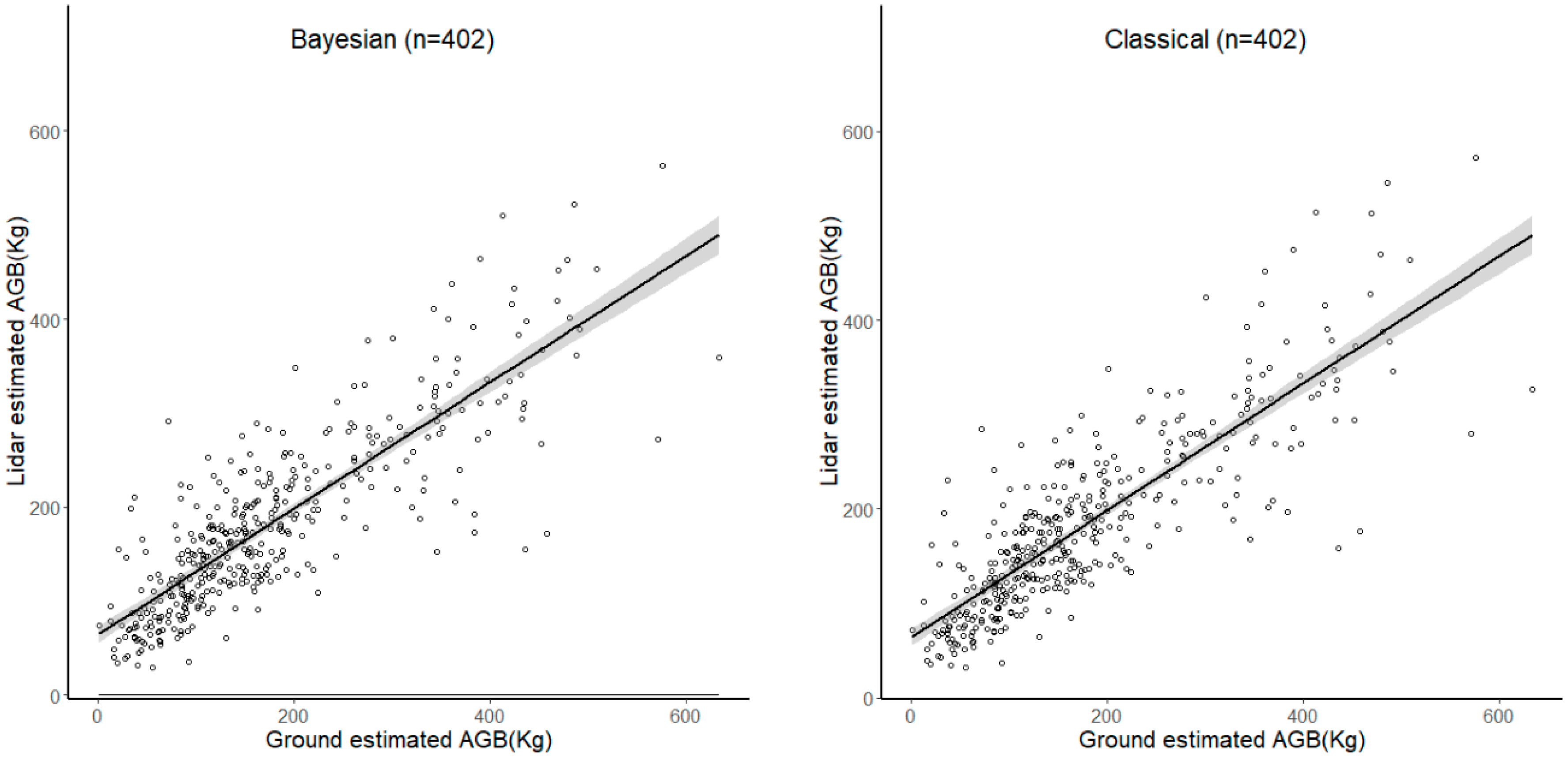
Figure 1 shows the correlations and residuals of AGB using the Bayesian method and the classical method when pooling the data. Both these plots show that the two methods performed well when modeling AGB. Also, the two plots from the two methods are very similar. However, as sample size decreased, the two methodologies produced large differences in R² and MAD. For example, when pooling the data, the R² of the Bayesian method was 0.5867, which was 2.587% larger than that of the classical method (0.5719). However, for a sample size of 39, the R² of the Bayesian method was 11.238% larger than that of the classical method (

Table 6. The accuracy of model II.3 using different methods (hierarchical Bayesian and NLME) to estimate the value of AGB (R²; MAD, mean absolute deviation).

Sample Size	Method	R2	MAD
10% (39)	Bayesian	0.8611	31.0571
	classical	0.7741	34.2188
25% (99)	Bayesian	0.7704	43.2709
	classical	0.7529	43.1827
50% (199)	Bayesian	0.7529	40.5010
	classical	0.7503	40.2283
75% (303)	Bayesian	0.7080	44.8375
	classical	0.7046	44.6531
100% (402)	Bayesian	0.5867	48.3125
	classical	0.5719	49.3627

). Similarly, although the MAD value from the Bayesian method was slightly smaller (2.172%) than that from the classical method using the whole data set, it was much smaller (16.62%) than that from the classical method for a sample size of 39 (Table 6).

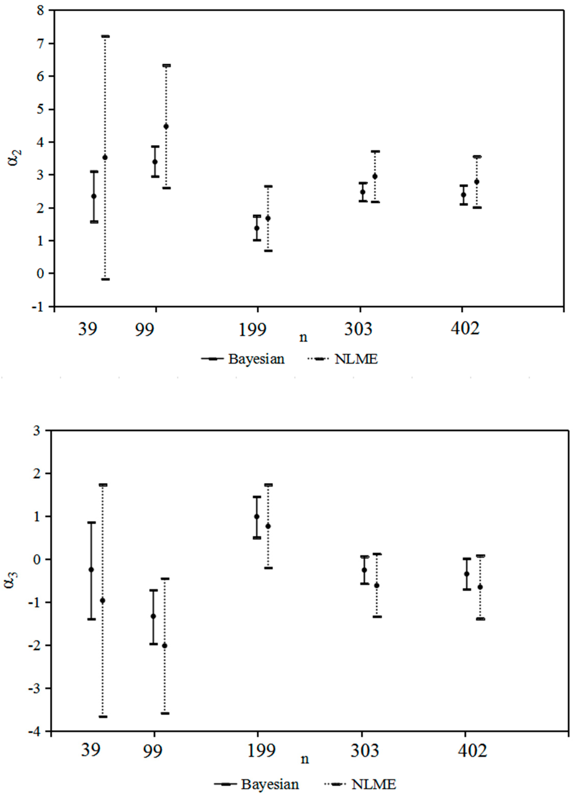
In addition, we found that parameter estimation through the Bayesian method was more stable than that through the classical method when using different sample sizes. For the parameter α₁, the parameter range was 0.027–0.281 for the Bayesian method and 0.007–0.167 for the classical method. In particular, when the sample size was 39, the estimate changed largely compared with that for the pooled data set using the classical method, which could also be seen in parameters α₂ and α₃ (Figure 2). In addition, we found that the classical approach always produced estimates in a wider range than the Bayesian approach (Figure 2).

4. Discussion and Conclusions

In this study, an individual tree DBH and AGB model was selected from seven DBH models and five AGB models using the Bayesian method on the basis of airborne LIDAR data. When selecting a model, we ensured that all models were compared at the same level and that the random effects of the parameters were considered in the same position. The criteria of model selection were the value of DIC and the results of the parameter stationarity test. When selecting the AGB model, the independent variable DBH was the LIDAR estimated DBH, which ensured that the selected AGB model took the correlation between DBH and AGB into account.

LIDAR has the ability to measure the forest structure, and it is a useful tool for obtaining canopy information [11]. This study used LIDAR to obtain the image data of our study area, then acquired individual tree information, including individual tree height and crown projection area, for model development. For aboveground biomass estimation, many studies have used LIDAR data. Næsset et al. [12] used LIDAR data for estimating the timber volume of forest stands. They obtained the LIDAR canopy height and canopy cover density for timber volume estimation, and they found that LIDAR data produced equal results to aerial photointerpretation, though different sites had large differences when estimating timber volume. Holmgren et al. [11] studied how to use LIDAR-derived data in regressive models for estimating the mean tree height and stem volume; the R² of mean tree height linear regression functions was between 0.89 and 0.91 and that for average stem volumes was between 0.82 and 0.9 when using the LIDAR mean tree height and LIDAR crown coverage area as variables. LIDAR is widely used in biomass prediction.

The study of forest biomass by the Bayesian method has been relatively less frequent than by the classical method. When the Bayesian method is compared to the classical method, an important difference is that the Bayesian method treats the parameters as random variables, while the classical method treats the parameters as fixed values; that is, the classical method treats the probability as the stable value of the frequency of a large number of repeated trials of events. Zapata-Cuartas et al. [14] used the existing biomass equation reported in the literature as the prior distribution, assuming that the information can be useful to probability distributions, and validated the larger R² in the Bayesian method. This study used a different approach to the prior distribution—we used the parameters estimated by NLME for the prior distribution and obtained the same results.

We compared the classical method and the Bayesian method in estimating DBH and AGB; the results show that parameter estimation using the Bayesian method had higher stability than that using the classical method, and the R² of the Bayesian method was higher than that of the classical method. Zianis et al. [17] also compared the two methods—they obtained a contrary result that the classical method was superior to the Bayesian method [17], but they did not compare the two methods on different sample sizes. In order to show that the Bayesian method is more accurate in estimating AGB for different sample sizes, we randomly sampled from the complete data set (Table 6). The data showed that the Bayesian method was more efficient than the classical method for different sizes of samples, which is the same as the result for the full data set. Zapata-Cuartas et al. [14] compared these two methods in the same way, and their results showed that for small sample sizes, the Bayesian method outperforms classical methods of least-square regression. Huang et al. [37] used the same method and showed that when the sample size is less than 50, we should use the Bayesian method to estimate aboveground biomass. Yao et al. [38] also presented a comparison of the Bayesian and classical methods—they found a more stable parameter value when using the Bayesian method. Thus, using the Bayesian method to estimate the aboveground biomass from small sample sizes is a good direction in biomass estimation. If classical methods are applied, especially with a small sample size, violation of statistical assumptions of error can lead to biased point estimates [20,39]. In addition, in this study, we have not taken into account the error propagation, thus a join model is perhaps a good method, and further studies are needed to solve the join model under the Bayesian framework for reducing the model uncertainties.

This study developed LIDAR DBH and LIDAR AGB models using the Bayesian method based on airborne LIDAR data. Previous studies have used the classical method to develop models and applied the classical method to airborne LIDAR data [9,10]. Fu et al. [1] developed a system to predict individual tree diameter and aboveground biomass using the classical method and compared two other widely used model structures (the classical method to estimate AGB depending on DBH and the classical method to estimate AGB not depending on DBH). The current article compared the classical method to the hierarchical Bayesian method, and the results of this study showed that the Bayesian method has higher R² and smaller MAD than the classical method for all sample sizes; thus, the Bayesian method was better than the classical method in estimating LIDAR DBH and LIDAR AGB for Picea crassifolia Kom. in northwestern China.

Overall, this study combined the advantages of the Bayesian method and airborne LIDAR data; that is, airborne LIDAR data are easier to obtain than conventional aboveground measurements, and the Bayesian method was proven to have greater accuracy than the classical method. In addition, the present study also provides a reference for modeling with a small sample size.

References

- Zhu, J.; Hu, H.; Tao, S.; Chi, X.; Li, P.; Jiang, L.; Ji, C.; Zhu, J.; Tang, Z.; Pan, Y.; et al. Carbon stocks and changes of dead organic matter in China’s forests. Nat. Commun. 2017, 8. [Google Scholar] [CrossRef]
- He, Q.; Chen, E.; An, R.; Li, Y. Above-ground biomass and biomass components estimation using Lidar data in a coniferous forest. Forests 2013, 4, 984–1002. [Google Scholar] [CrossRef]
- Fu, L.; Liu, Q.; Sun, H.; Wang, Q.; Li, Z.; Chen, E.; Pang, Y.; Song, X.; Wang, G. Development of a system of compatible individual tree diameter and aboveground biomass prediction models using error-in-variable regression and airborne Lidar data. Remote Sens. 2018, 10, 325. [Google Scholar] [CrossRef]
- Fu, L.; Lei, Y.; Wang, G.; Bi, H.; Tang, S.; Song, X. Comparison of seemingly unrelated regressions with error-in-variable models for developing a system of nonlinear additive biomass equations. Trees 2016, 30, 839–857. [Google Scholar] [CrossRef]
- Nelson, R.; Krabill, W.; Tonelli, J. Estimating forest biomass and volume using airborne laser data. Remote Sens. Environ. 1988, 24, 247–267. [Google Scholar] [CrossRef]
- Neumann, M.; Saatchi, S.S.; Ulander, L.M.H.; Fransson, J.E.S. Assessing performance of l- and p-band polarimetric interferometric SAR data in estimating boreal forest above-ground biomass. IEEE Trans. Geosci. Remote Sens. 2012, 50, 714–726. [Google Scholar] [CrossRef]
- Tian, X.; Su, Z.; Chen, E.; Li, Z.; van der Tol, C.; Guo, J.; He, Q. Estimation of forest above-ground biomass using multi-parameter remote sensing data over a cold and arid area. Int. J. Appl. Earth Obs. 2012, 14, 160–168. [Google Scholar] [CrossRef]
- Zheng, C.; Mason, E.G.; Jia, L.; Wei, S.; Sun, C.; Duan, J. A single-tree additive biomass model of Quercus variabilis Blume forests in north China. Trees 2015, 29, 705–716. [Google Scholar] [CrossRef]
- Zianis, D.; Muukkonen, P.; Mäkipää, R.; Mencuccini, M. Biomass and stem volume equations for tree species in Europe. Silva Fenn. Monogr. 2005, 4, 1–63. [Google Scholar]
- Zianis, D.; Mencuccini, M. On simplifying allometric analyses of forest biomass. For. Ecol. Manag. 2004, 187, 311–332. [Google Scholar] [CrossRef] [Green Version]
- Holmgren, J.; Nilsson, M.; Olsson, H. Estimation of tree height and stem volume on plots using airborne laser scanning. For. Sci. 2003, 49, 419–428. [Google Scholar]
- Næsset, E. Estimating timber volume of forest stands using airborne laser scanner data. Remote Sens. Environ. 1997, 61, 246–253. [Google Scholar] [CrossRef]
- Hansen, E.; Ene, L.; Mauya, E.; Patocka, Z.; Mikita, T.; Gobakken, T.; Næsset, E. Comparing empirical and semi-empirical approaches to forest biomass modelling in different biomes using airborne laser scanner data. Forests 2017, 8, 170. [Google Scholar] [CrossRef]
- Zapata-Cuartas, M.; Sierra, C.A.; Alleman, L. Probability distribution of allometric coefficients and Bayesian estimation of aboveground tree biomass. For. Ecol. Manag. 2012, 277, 173–179. [Google Scholar] [CrossRef]
- Zell, J.; Bösch, B.; Kändler, G. Estimating above-ground biomass of trees: Comparing Bayesian calibration with regression technique. Eur. J. For. Res. 2014, 133, 649–660. [Google Scholar] [CrossRef]
- Zhang, X.; Duan, A.; Zhang, J.; Xiang, C. Estimating tree height-diameter models with the Bayesian method. Sci. World J. 2014, 2014, 683–691. [Google Scholar] [CrossRef] [PubMed]
- Zianis, D.; Spyroglou, G.; Tiakas, E.; Radoglou, K. Bayesian and classical models to predict above ground tree biomass allometry. For. Sci. 2016, 62, 247–259. [Google Scholar]
- Farid, A.; Goodrich, D.; Sorooshian, S. Using airborne Lidar to discern Age classes of cottonwood trees in a riparian Area. West. J. Appl. For. 2006, 21, 149–158. [Google Scholar]
- Hauglin, M.; Gobakken, T.; Astrup, R.; Ene, L.; Næsset, E. Estimating single-tree crown biomass of Norway spruce by airborne laser scanning: A comparison of methods with and without the use of terrestrial laser scanning to obtain the ground reference data. Forests 2014, 5, 384–403. [Google Scholar] [CrossRef]
- Kuyah, S.; Sileshi, G.; Rosenstock, T. Allometric models based on Bayesian frameworks give better estimates of aboveground biomass in the Miombo woodlands. Forests 2016, 7, 13. [Google Scholar] [CrossRef]
- Picard, N.; Henry, M.; Mortier, F.; Trotta, C.; Saint-Andre, L. Using Bayesian model averaging to predict tree aboveground biomass in tropical moist forests. For. Sci. 2011, 58, 15–23. [Google Scholar] [CrossRef]
- Hoeting, J.A.; Madigan, D.; Raftery, A.E.; Volinsky, C.T. Bayesian model averaging: A tutorial. Stat. Sci. 1999, 14, 382–417. [Google Scholar]
- Olubusoye, O.; Okonkwo, O. Choice of priors and variable selection in Bayesian regression. J. Asian Sci. Res. 2018, 2, 354–377. [Google Scholar]
- Tenneson, K. Development of a regional Lidar-derived forest inventory model with Bayesian model averaging for use in ponderosa pine and mixed conifer forests in Arizona and new Mexico, USA. Remote Sens. 2018, 10, 442. [Google Scholar] [CrossRef]
- Wang, J.; Che, K.; Fu, H.; Chang, X.; Song, C.; He, H. Study on biomass of water conservation forest on north Slope of Qilian mountains. J. Fujian Coll. For. 1998, 18, 319–323. (In Chinese) [Google Scholar]
- Bi, H.; Fox, J.; Li, Y.; Lei, Y.; Pang, Y. Evaluation of nonlinear equations for predicting diameter from tree height. Can. J. For. Res. 2012, 42, 789–806. [Google Scholar] [CrossRef]
- Yang, R.C.; Kozak, A.; Smith, J.H.G. The potential of Weibull-type functions as a flexible growth curve. Can. J. For. Res. 1978, 8, 424–431. [Google Scholar] [CrossRef]
- Ruark, G.A.; Martin, G.L.; Bockheim, J.G. Comparison of constant and variable allometric ratios for estimating Populus tremuloides biomass. For. Sci. 1987, 33, 294–300. [Google Scholar]
- Zhang, X.; Duan, A.; Zhang, J. Tree biomass estimation of Chinese fir (Cunninghamia lanceolata) based on Bayesian method. PLoS ONE 2013, 8, e79868. [Google Scholar] [CrossRef]
- Ellison, A.M. Bayesian inference in ecology. Ecol. Lett. 2004, 7, 509–520. [Google Scholar] [CrossRef] [Green Version]
- Zhang, X.; Zhang, J.; Duan, A. A hierarchical Bayesian model to predict self-thinning line for Chinese Fir in southern China. PLoS ONE 2015, 10. [Google Scholar] [CrossRef] [PubMed]
- Zhang, X.; Zhang, J.; Duan, A. Tree-height growth model for Chinese fir plantation based on Bayesian method. Sci. Silvae Sin. 2014, 50, 69–75. (In Chinese) [Google Scholar]
- Heidelberger, P.; Welch, P.D. Simulation run length control in the presence of an initial transient. Opns. Res. 1983, 31, 1109–1144. [Google Scholar] [CrossRef]
- Heidelberger, P.; Welch, P.D. A spectral method for confidence interval generation and run length control in simulations. Commun. ACM 1981, 24, 233–245. [Google Scholar] [CrossRef]
- Kipiński, L.; König, R.; Sielużycki, C.; Kordecki, W. Application of modern tests for stationarity to single-trial meg: Data transferring powerful statistical tools from econometrics to neuroscience. Biol. Cybern 2011, 105, 183–195. [Google Scholar] [CrossRef] [PubMed]
- SAS Institute, Inc. SAS/STAT 9.3 User’s Guide; SAS Institute, Inc.: Cary, NC, USA, 2011; 3316p. [Google Scholar]
- Huang, X.; Chen, D.; Sun, X.; Zhang, S. Estimation on above-ground tree biomass based on probability distribution of allometric parameters. Sci. Silvae Sin. 2014, 50, 34–41. (In Chinese) [Google Scholar]
- Yao, D. Individual Tree Growth Model for Mongolia Oak Forest with Bayesian Statistical Inference. Master’s Thesis, Chinese Academy of Forestry, Beijing, China, 2015. (In Chinese). [Google Scholar]
- Sileshi, G.W. A critical review of forest biomass estimation models, common mistakes and corrective measures. For. Ecol. Manag. 2014, 329, 237–254. [Google Scholar] [CrossRef]
Figure 1.
Correlation (95% interval) and residual plots for aboveground biomass (AGB) through the hierarchical Bayesian and classical (NLME, nonlinear mixed effects model) methods (From top to bottom: Correlation for AGB by hierarchical Bayesian and classical method; residual plots for AGB by hierarchical Bayesian and classical method).
Figure 2.
Parameter comparison with 95% intervals between the hierarchical Bayesian method and the classical method (NLME) using different sample sizes.