Article

NWCSAF High Resolution Winds (NWC/GEO-HRW) Stand-Alone Software for Calculation of Atmospheric Motion Vectors and Trajectories

1
Satellite Application Facility on Support to Nowcasting and Very Short Range Forecasting (NWCSAF), Agencia Estatal de Meteorología (AEMET), Leonardo Prieto Castro 8, 28040 Madrid, Spain
2
Satellite Application Facility on Support to Nowcasting and Very Short Range Forecasting (NWCSAF), GMV, Isaac Newton 11, 28760 Tres Cantos, Madrid, Spain
*
Author to whom correspondence should be addressed.
Remote Sens. 2019, 11(17), 2032; https://doi.org/10.3390/rs11172032
Submission received: 19 July 2019 / Revised: 23 August 2019 / Accepted: 24 August 2019 / Published: 29 August 2019
(This article belongs to the Special Issue Satellite-Derived Wind Observations)

Abstract

:
The High Resolution Winds (NWC/GEO-HRW) software is developed by the EUMETSAT Satellite Application Facility on Support to Nowcasting and Very Short Range Forecasting (NWCSAF). It is part of a stand-alone software package for the calculation of meteorological products with geostationary satellite data (NWC/GEO). NWCSAF High Resolution Winds provides a detailed calculation of Atmospheric Motion Vectors (AMVs) and Trajectories, locally and in near real time, using as input geostationary satellite image data, NWP model data, and OSTIA sea surface temperature data. The whole NWC/GEO software package can be obtained after registration at the NWCSAF Helpdesk, www.nwcsaf.org, where users also find support and help for its use. NWC/GEO v2018.1 software version, available since autumn 2019, is able to process MSG, Himawari-8/9, GOES-N, and GOES-R satellite series images, so that AMVs and trajectories can be calculated all throughout the planet Earth with the same algorithm and quality. Considering other equivalent meteorological products, in the ‘2014 and 2018 AMV Intercomparison Studies’ NWCSAF High Resolution Winds compared very positively with six other AMV algorithms for both MSG and Himawari-8/9 satellites. Finally, the Coordination Group for Meteorological Satellites (CGMS) recognized in its ‘2012 Meeting Report’: (1) NWCSAF High Resolution Winds fulfills the requirements to be a portable stand-alone AMV calculation software due to its easy installation and usability. (2) It has been successfully adopted by some CGMS members and serves as an important tool for development. It is modular, well documented, and well suited as stand-alone AMV software. (3) Although alternatives exist as portable stand-alone AMV calculation software, they are not as advanced in terms of documentation and do not have an existing Helpdesk.

Graphical Abstract

1. Introduction

The Satellite Application Facility on Support to Nowcasting and very short range forecasting (NWCSAF) is a consortium inside the EUMETSAT Satellite Application Facility (SAF) network, conformed by five National Meteorological Services: AEMET/Agencia Estatal de Meteorología of Spain, MF/Météo-France, ZAMG/Zentralanstalt für Meteorologie und Geodynamik of Austria, SMHI/Sveriges Meteorologiska och Hydrologiska Institut of Sweden, and ANM/Administraţia Naţională de Meteorologie of Romania. The work of the Consortium started in 1997.
The main objective and requirement of the NWCSAF [1] is to produce two stand-alone software packages, which calculate in near real time meteorological products from geostationary and polar satellite data (NWC/GEO and NWC/PPS).
These software packages are installed locally at the user’s site, to enhance the nowcasting and very short range forecasting (i.e., the weather forecasting up to a period of 12 h [2]). As stand-alone software packages, they contain all the elements for the calculation of the products without the need of any other elements, beyond the corresponding input data. The NWCSAF also supports its users on the generation and application of the products.
NWC/GEO v2018.1 software package, available since autumn 2019, calculates the following seven types of meteorological products considering images of MSG, Himawari-8/9, and GOES-N and GOES-R satellite series (GOES-13 and subsequent ones), covering the whole Earth in the areas which can be observed with geostationary satellites.
  • Four cloud products: Cloud Mask (CMA); Cloud Type (CT); Cloud Top Temperature, Height and Pressure (CTTH); and Cloud Microphysics (CMIC). The last product provides cloud phase, cloud effective radius, cloud optical thickness, and liquid/ice water path.
  • Two pairs of precipitation products: Precipitating Clouds (PC and PC-Ph), providing the probability of precipitation for a cloudy pixel, and Convective Rainfall Rate (CRR and CRR-Ph), providing instant and hourly values of precipitation, more suitably for convective clouds. In both pairs of products, the second product makes use of the Cloud Microphysics (CMIC) product in its algorithm, while the first product does not make use of this information.
  • Two convection products: Convection Initiation (CI), providing the probability for a cloudy pixel to become a thunderstorm, and Rapid Developing Thunderstorms (RDT), tracking and monitoring convective systems highlighting many of their properties.
  • One clear air product: imaging Satellite Humidity and Instability (iSHAI). This product provides for clear air pixels vertical profiles of humidity, temperature and ozone, precipitable water available in the total column and in three vertical layers, and several instability indices.
  • Three conceptual model products: Automatic Satellite Image Interpretation (ASII), Tropopause Folding (ASII-TF), and Gravity waves (ASII-GW). These products interpret the satellite image in terms of conceptual models; the two last ones related to turbulence.
  • One extrapolation product: Extrapolated Imagery (EXIM). This product forecasts satellite imagery or other NWC/GEO products, considering kinematic extrapolation.
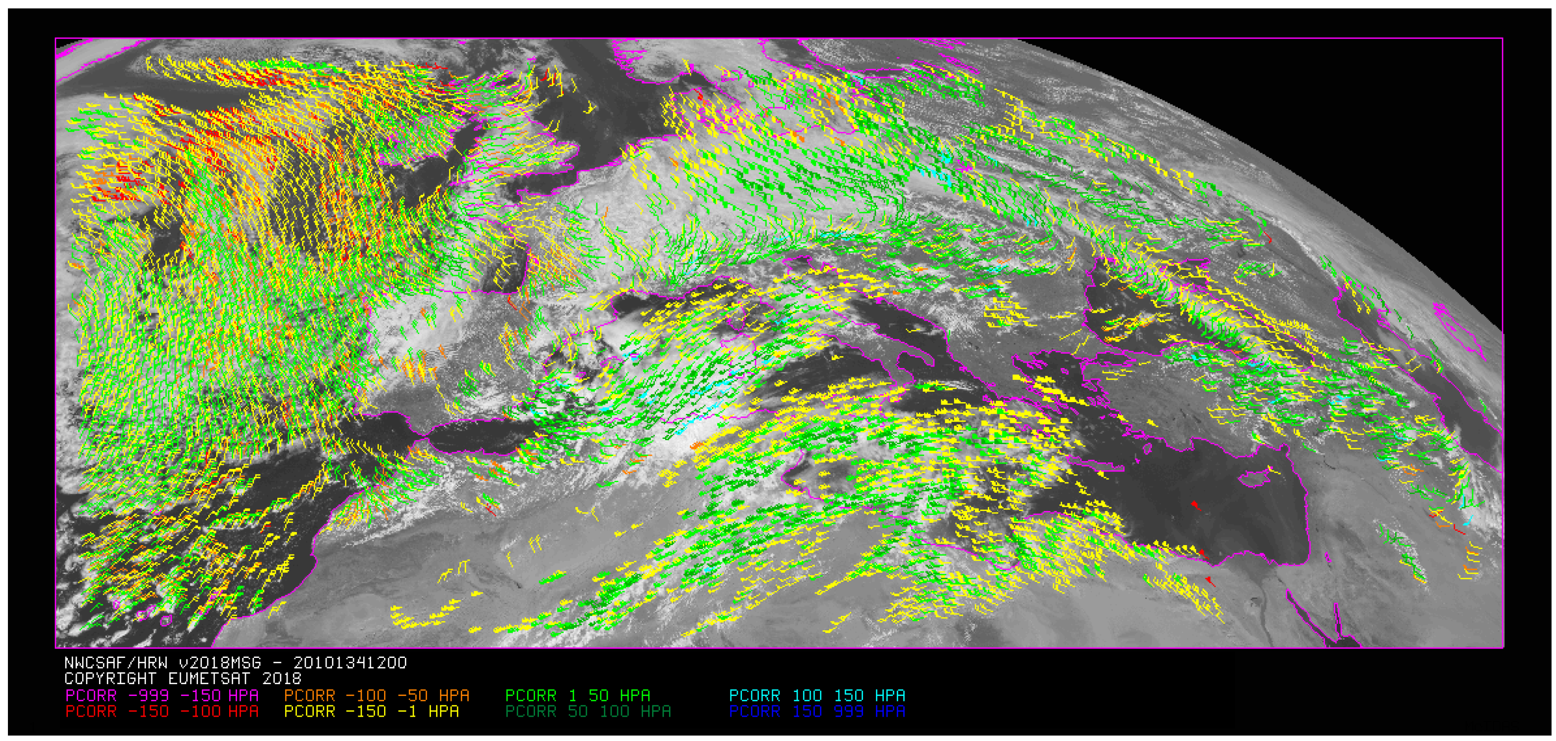
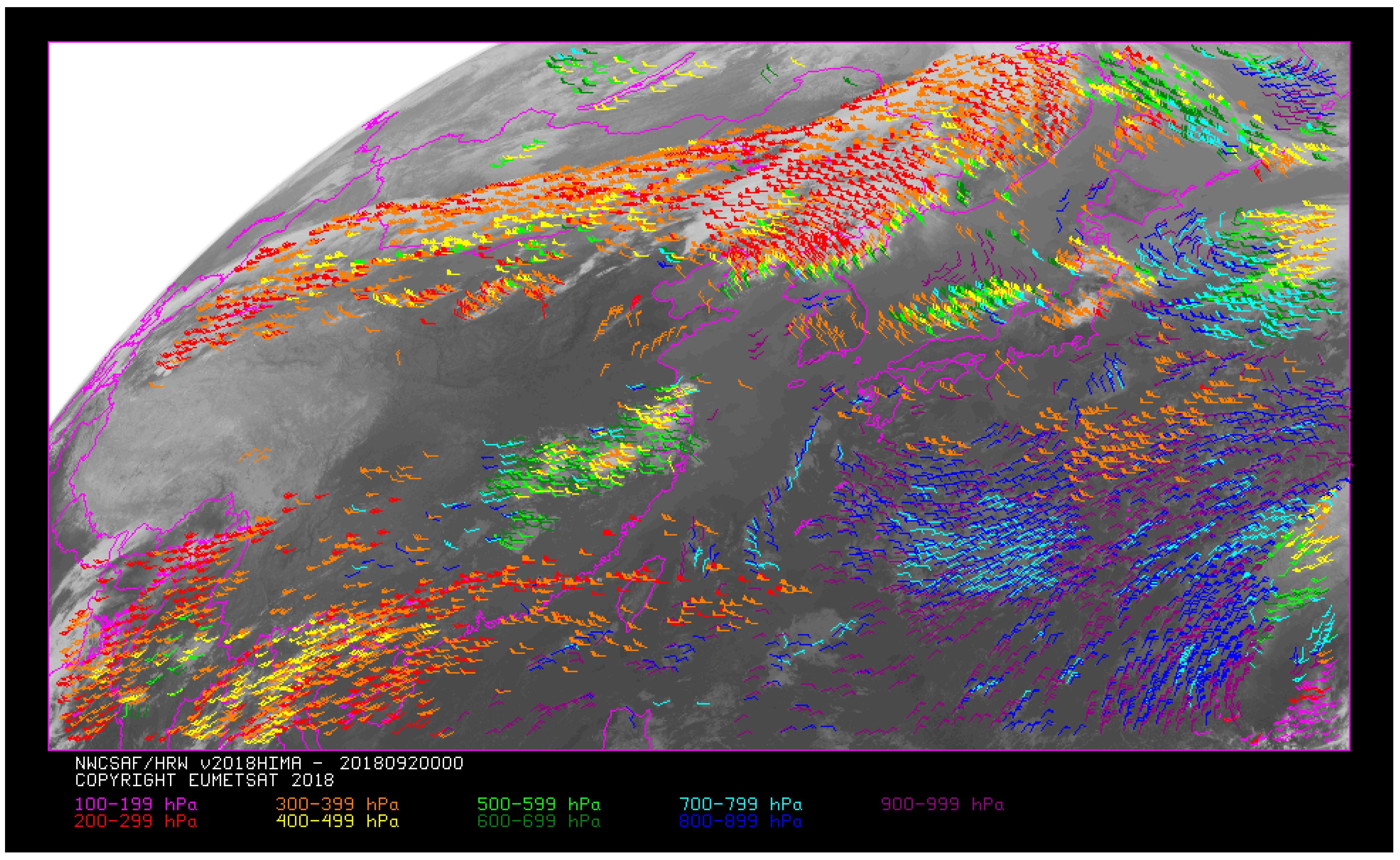
  • One AMV product: High Resolution Winds (HRW). This product calculates atmospheric motion vectors (AMVs) and Trajectories, through the displacement of cloudiness and humidity features in successive satellite images.
A full description and validation of the NWCSAF High Resolution Winds (NWC/GEO-HRW) product (from now on, NWC/GEO-HRW v2018.1 product included in NWC/GEO v2018.1 software package), is shown in this paper.
An atmospheric motion vector (AMV) is the horizontal displacement between two Earth positions in two satellite images, of a square segment of n × n pixels called ‘tracer’. A ‘trajectory’ is the path defined by the displacement of the same tracer throughout several satellite images.
Examples of atmospheric motion vectors (AMVs) and trajectories obtained for a same slot with NWC/GEO-HRW product are shown in Figure 1 and Figure 2.
A tracer is defined through a specific cloudiness feature in visible, infrared or water vapor images (cloudy tracer), or through a specific humidity feature in cloudless areas in water vapor images (clear air tracer). The tracer has a fixed size in pixels. Tracers are identified in an initial image and tracked in a later image, obtaining from their displacement between those images the atmospheric motion vectors (AMVs).
HRW product includes pressure level information, which locates in the vertical dimension the calculated AMVs and trajectories, and also a quality control flagging, which gives an indication of the error in probabilistic terms, with auxiliary indicators about how the product was determined.
AMVs and trajectories are calculated 24 h a day, considering the displacement of tracers in:
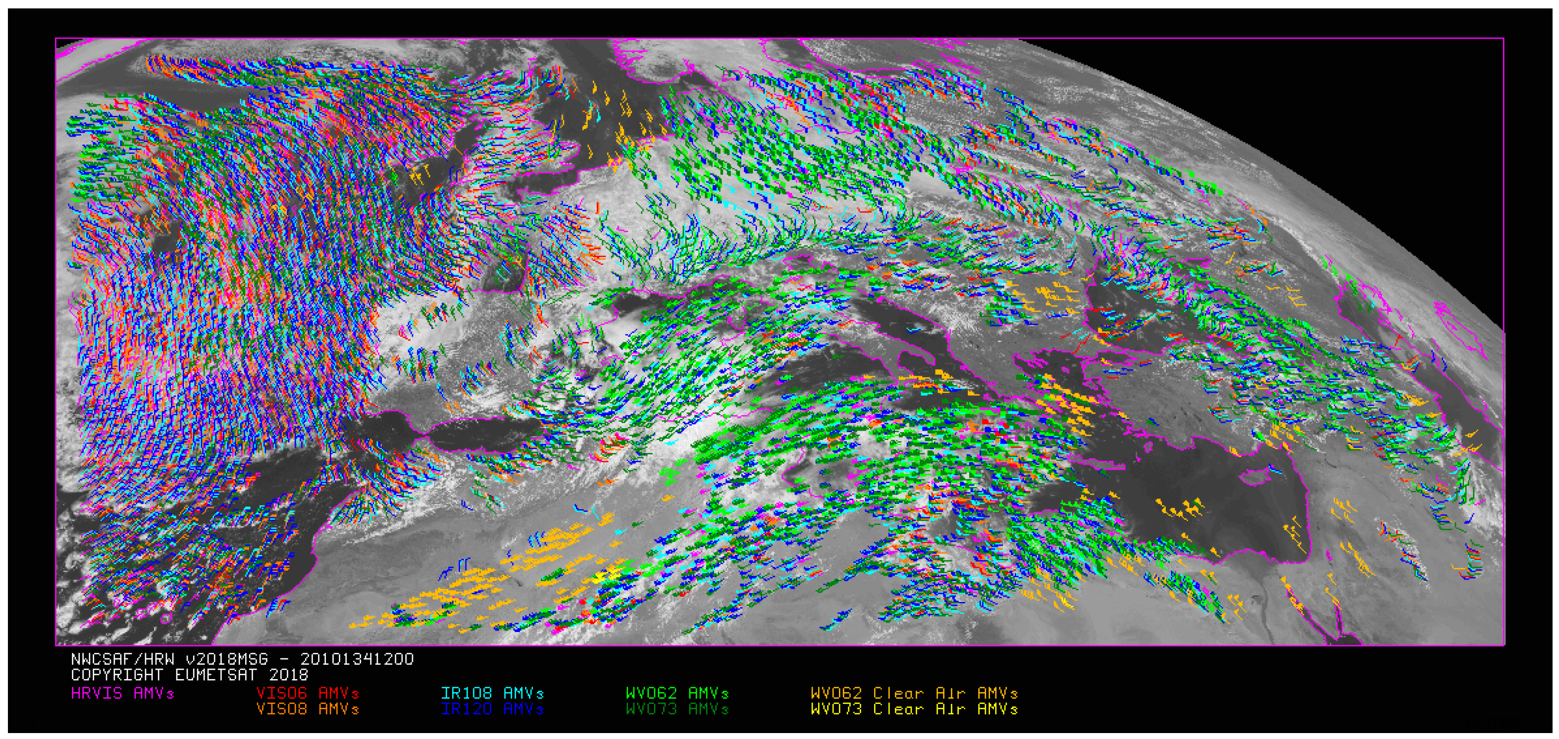
  • Up to seven MSG/SEVIRI channel images every 15 min (in ‘nominal scan mode’) or 5 min (in ‘rapid scan mode’): HRVIS (band 12), VIS06 (band 1), VIS08 (band 2), IR108 (band 9), IR120 (band 10), WV62 (band 5), WV73 (band 6).
  • Up to six Himawari-8/9/AHI channel images, every 10 min: VIS06 (band 3), VIS08 (band 4), IR112 (band 14), WV62 (band 8), WV70 (band 9), WV74 (band 10).
  • Up to three GOES-N/IMAGER channel images every 15 min (in the continental United States region) or 30 min (in the North America region): VIS07 (band 1), IR107 (band 4), WV65 (band 3).
  • Up to six GOES-R/ABI channel images every 10 or 15 min: VIS06 (band 2), VIS08 (band 3), IR112 (band 14), WV62 (band 8), WV70 (band 9), WV74 (band 10).
AMVs are associated with the horizontal wind in the atmosphere. Exceptions exist to this, related generally to clouds which are blocked or whose flow is affected by orography, or to lee wave clouds with atmospheric stability near mountain ranges. However, these exceptions are identified and discarded.
In order to forecast the weather, conventional observations are sparse, whereas satellite-based observations provide near global coverage at regular time intervals. This way, the derivation of AMVs from satellite images is an important source of global wind information, especially over the oceans and in remote continental areas. Considering this, NWCSAF High Resolution Winds (NWC/GEO-HRW) is useful in nowcasting and forecasting applications, in synergy with other data available to the forecaster. For example, in the monitoring of the general atmospheric flow, of small-scale circulation and wind singularities, of convergence at low levels or divergence at the top of developed systems, and in the watch and warning of dangerous wind situations. It can also be used in the form of objectively derived fields, assimilated in numerical weather prediction models together with many other data, or used as an input in analysis and forecast applications.
For the research community, NWCSAF High Resolution Winds (NWC/GEO-HRW) is also a ready-to-go starting point for the derivation of winds from satellite measurements. It can serve as focal point for sharing and comparing code among different research groups, which could lead to a better understanding of AMVs, future algorithm enhancements, and improvements in the performance of operationally derived AMVs.
Finally, during discussions at the 38th and 39th CGMS meetings in 2010 and 2011, and also at the 10th International Winds Workshop in 2012 [3], the need to have a stand-alone and user-friendly AMV calculation software was emphasized. One of the arguments for this stand-alone AMV calculation software was to provide both AMV and Research communities a tool facilitating the research, testing and comparison of new AMV developments (which could improve the general quality of extracted AMVs). Another important argument was to be able to calculate AMVs and trajectories all throughout the Earth with the same algorithm and quality. Both arguments are currently fulfilled by NWCSAF High Resolution Winds (NWC/GEO-HRW) product.
In case of interest on using NWC/GEO software package and NWC/GEO-HRW product, all National Meteorological Services within EUMETSAT Member and Cooperating States are automatically considered as potential NWCSAF users. All other organizations may also apply to become NWCSAF users, contacting through email at [email protected]. All current applicants have become NWCSAF users without restrictions.

2. Materials and Methods

NWCSAF High Resolution Winds (NWC/GEO-HRW) product is designed in a modular way in the form of C and Fortran functions. These functions are available to the NWCSAF user, and are fully commented step by step, so that they are easy to understand. The whole process includes the following parts, explained in detail.

2.1. Preprocessing

During the preprocessing, the following parameters are extracted for use by NWC/GEO-HRW product:
  • Reflectances (normalized, taking into account the distance to the Sun) for all pixels in the processing region, in the visible images on which tracers are calculated and tracked.
  • Brightness temperatures for all pixels in the processing region, in the infrared and water vapor images on which tracers are calculated and tracked.
  • Radiances for all pixels in the processing region, in the images on which tracers are calculated and tracked, for MSG/IR108 and WV62, GOES-N/IR107 and WV65, or Himawari-8/9 or GOES-R/IR112 and WV62 satellite channels.
  • NWP profiles for all pixels in the processing region, with the satellite lowest resolution, for the following variables: temperature forecast, geopotential forecast, wind component forecast, and wind component analysis.
  • Latitudes and longitudes, and solar and satellite zenith angles, for all pixels in the processing region, in the images on which tracers are calculated and tracked (calculated by NWC/GEO).
  • NWC/GEO-CT cloud type; NWC/GEO-CTTH cloud top temperature, pressure and height; and NWC/GEO-CMIC cloud phase, liquid water path and ice water path outputs, for all pixels in the processing region, in the image on which tracers are tracked.
  • High resolution global OSTIA data for Sea Surface Temperature and Local Estimated Error [4], obtainable such as described in [5]. Although not directly used by NWC/GEO-HRW product, it is used for the processing of the NWC/GEO-Cloud products.
Here, only the satellite data for the requested satellite channels, and the NWP temperature data with a minimum number of levels are mandatory (a configurable parameter with a default value of 4). All other data contribute to a higher number of AMVs and trajectories and a better quality of the output data. The option to calculate AMVs and trajectories without NWP data is not available, since the amount and quality of data provided would be significantly worse.
The satellite data are to be provided in full resolution uncompressed original SEVIRI/HRIT data (for MSG satellite series), AHI/HSD data (for Himawari-8/9 satellite series), IMAGER/GVAR data (for GOES-N satellite series), or ABI/NetCDF data (for GOES-R satellite series). For processing, the normalized reflectances and brightness temperatures from these satellite data are scaled to ‘brightness values’: integer values from 0 to 255, in so-called ‘image matrices’.
NWP data are to be provided with a horizontal resolution of at least 0.5°, and a temporal resolution of at most 6 h (a time step of at most 3 h is preferred). ECMWF NWP model is used as default option, but other NWP models have also been used by different NWCSAF users (being the most common Météo-France ARPEGE and NOAA/NCEP GFS NWP models). NWP data are then temporally interpolated at each image and spatially interpolated at each pixel in the processing region, for their use by HRW product.

2.2. Tracer Search

The process of HRW product starts with the calculation of ‘tracers’ throughout the processing region in an initial image (as already said, square segments of n × n pixels, used as initial positions of an AMV and trajectory, and identified by a specific cloudiness feature or humidity feature). The geographical region, and the latitude and longitude limits for the calculation of AMVs and trajectories can be specified with configurable parameters.
With the default configuration, the definition of new ‘tracer locations’ starts at the location of all ‘tracking centers’ related to valid AMVs in the previous round, when they are available. A set of ‘persistent tracers’ can so successively be defined and tracked in several images, and the progressive locations of the tracers throughout the time define the ‘trajectories’. For this, it is necessary that the conditions implied by the ‘tracer method’ used for the determination of the tracer in the initial image, keep on being valid throughout all the images.
If no tracers are available for the calculation from a previous round of HRW product, the tracer calculation is the only process which is activated for the first image. Once tracers from a previous run identified as initial image are available and AMVs and Trajectories have been calculated, the following tracer calculation processes are activated as the final step of each HRW product run.
Two computation methods are applied for the calculation of new tracers: ‘gradient method’ and ‘tracer characteristics method’. Both define a tracer optimizing its location in the vicinity of the ‘starting locations’ (defined at specific distances from each other). Gradient method is by far more efficient in computing terms. Tracer characteristics method is more specific: it defines more tracers in empty areas with a longer but still reasonable computing time.
These tracer computation methods are used one after the other in two different tracer selection strategies throughout the region: the ‘single scale procedure’ (in which one scale of tracers is calculated), and the ‘two scale procedure’ (in which two different scales of tracers are calculated: ‘basic scale’ and ‘detailed scale’).
A single scale procedure calculating only basic tracers with a line and column tracer size of 24 pixels is proposed as the default configuration. A tracer size of 24 pixels for basic tracers and 12 pixels for detailed tracers is proposed as the baseline for the two-scale procedure. The line and column tracer size in pixels can be defined through configurable parameters. However, HRW product is defined to work with square shaped tracers, so similar values for the line and column tracer size are kept for the processing.
These resolutions define different tracer scales between 48 to 96 km at subsatellite point (in the basic lowest resolution image scale) and 6 to 12 km at subsatellite point (in the detailed highest resolution image scale), with the high values related to GOES-N satellite series and the low values related to Himawari-8/9 and GOES-R satellite series; between ‘mesoscale ß’ and ‘mesoscale γ’ meteorological dimensions.
The nominal observation frequency of 10–30 min is enough to track the majority of features with these sizes, although in some cases like small cumulus over land, the lifecycle might be a bit short for this image frequency. The use of HRW product in ‘rapid scan mode’ with MSG satellites can improve the results with tracers of this small size.

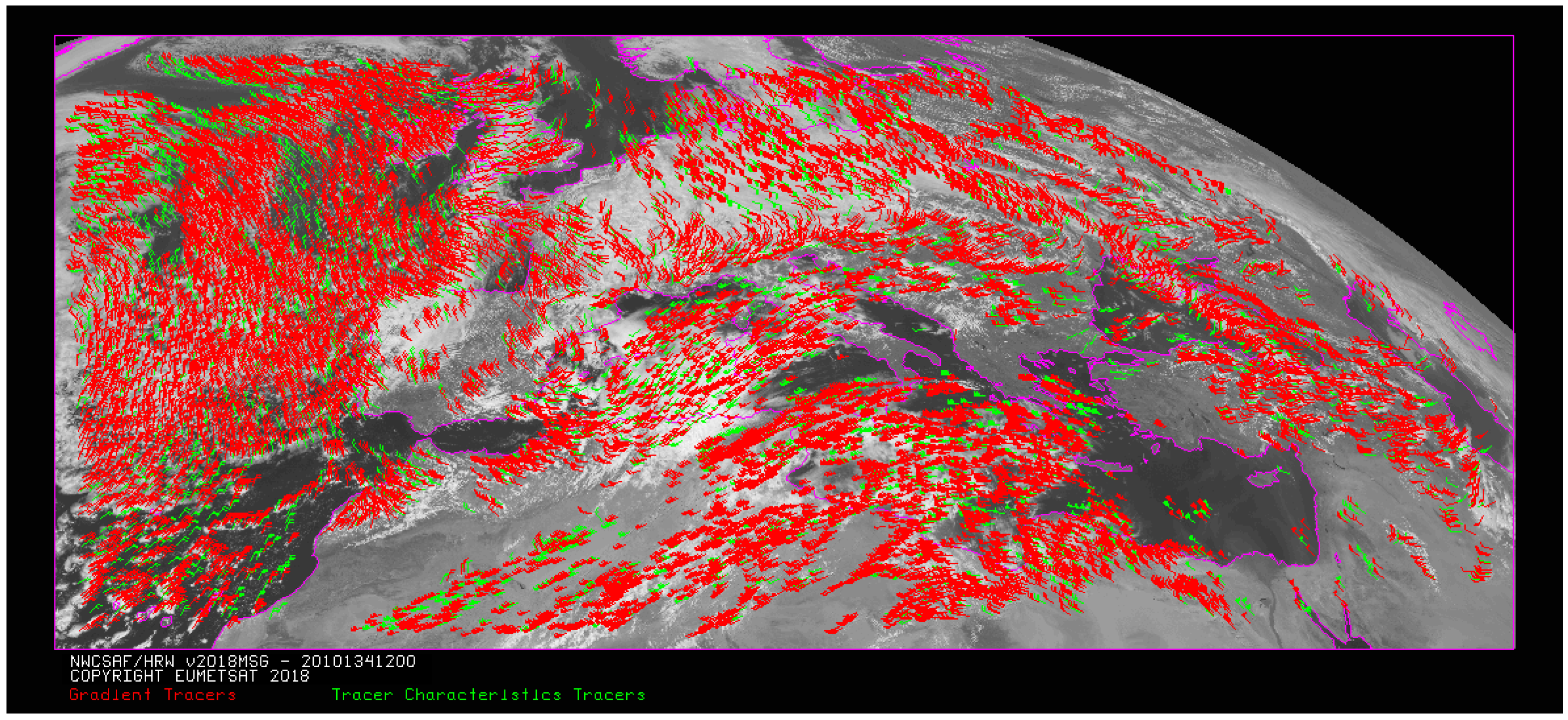
2.2.1. First Tracer Search Method: Gradient Method

Starting from the northwestern corner of the image in the processing region, tracer locations are defined with ‘gradient method’. This method is similar to the one defined by Hayden & Merrill [6]. It has the following steps:
  • To look for a brightness value (identified as any of the pixel values of the corresponding image matrix, inside a tracer candidate located at a starting location), greater than 120 (in visible cases) or smaller than 240 (in the other cases). This parameter is configurable.
  • To verify if a contrast exists between the maximum and minimum brightness value in the tracer candidate, greater than 60 (in visible cases) or greater than 48 (in the other cases). This parameter is also configurable.
  • To compute inside the tracer candidate the value and location of the maximum gradient |Δbrightness(Δx) + Δbrightness(Δy)|, considering a distance of 5 pixels in both line and column directions. This maximum gradient cannot be located on the edges of the tracer candidate.
If all previous processes have been successful, a valid tracer is defined at the location of the maximum gradient. In the default configuration of HRW v2018.1 product, the starting location for the subsequent tracer is established by a distance between tracers of 24 km, or 12 km if the tracer is related to a low or very low cloud. This way, the spatial separation of AMVs and Trajectories related to these low-level cloud types is narrower than the one for the other ones. This has been a request of NWCSAF users to increase the proportion of AMVs located at low levels.
If one failure occurs in the definition of a tracer location with ‘gradient method’, the distance to the next possible tracer is reduced to a half. Two consecutive failures defining a tracer location identify a ‘coverage hole’.

2.2.2. Second Tracer Search Method: Tracer Characteristics Method

The centers of coverage holes are the starting locations for the tracer search in a second iteration with the ‘tracer characteristics method’. It is based on new development. It is useful especially in the visible cases, where many potential tracers can present fainter edges because of cloudiness at different levels, with a similar reflectance. The method evaluates tracer candidates at increasing distances from each coverage hole (every 3 lines and columns, up to a maximum distance of 12 pixels). Two tests are here applied in sequence, so that a valid tracer can be defined:
(1) Frontier definition in the brightness histogram test:
It includes two parts, based on the histogram classification of the ‘brightness values’ of the pixels in a tracer candidate. In the first part, a significant contrast in the brightness values is to be found through the centiles of the histogram (CENT_nn%):
  • CENT_10% > 0.
  • CENT_90% ≥ 114 (visible cases); CENT_10% ≤ 252 (other cases).
  • CENT_97%-CENT_03% ≥ 20 if CENT_97% ≥ 150; ≥ 30 if CENT_97% < 150 (visible cases).
  • CENT_97%-CENT_03% ≥ 30 if CENT_03% ≤ 180; ≥ 50 if CENT_03% > 180 (other cases).
In the second part of this test, one significant ‘frontier’ is to be found in the brightness value histogram for the tracer candidate. The frontier is defined as the location of the deepest minimum in the brightness histogram, binned in groups of three brightness values. This frontier defines a group of ‘bright pixels’ (brighter than the frontier) and a group of ‘dark pixels’ (darker than the frontier).
(2) Big pixel brightness variability test:
The tracer candidate is now considered as a coarse structure of 4 × 4 ‘big pixels’, to be classified according to the brightness values of the respective pixel population. Three classes are possible:
  • CLASS_0: ‘dark big pixel’ (<30% of its pixels are ‘bright pixels’).
  • CLASS_2: ‘bright big pixel’ (>70% of its pixels are ‘bright pixels’).
  • CLASS_1: ‘undefined big pixel’ (intermediate case).
To avoid the use of tracers based on too faint features, it is requested that both CLASS_0 and CLASS_2 classes occur at least once in the 4 × 4 big pixel matrix, while the incidence of CLASS_1 being less than twice the less frequent of the other ones.
The 4 × 4 big pixel matrix is then checked for enough brightness variability. At least two CLASS_0 to CLASS_2 or CLASS_2 to CLASS_0 transitions must exist along three of the four main directions in the 4 × 4 big pixel matrix: rows, columns, ascending diagonal directions, and descending diagonal directions. For this, all linear arrays are checked in the row and column directions, while linear arrays with at least three elements are checked in the diagonal directions.

2.2.3. Condition on the Tracer Closeness

No tracer is retained if it is found too close to a previously computed one (‘closeness threshold’). Therefore, each time a tracer is computed, all pixels located nearer than this closeness threshold are added to a ‘pixel exclusion matrix’, and excluded as potential tracer locations.
An additional condition is verified, through which all pixels inside a tracer must have a satellite zenith angle (and a solar zenith angle in the case of visible channels) smaller than a maximum threshold (configurable parameters, 80° and 87° respectively). This guarantees that the illumination and satellite visualization conditions are good enough for the process.

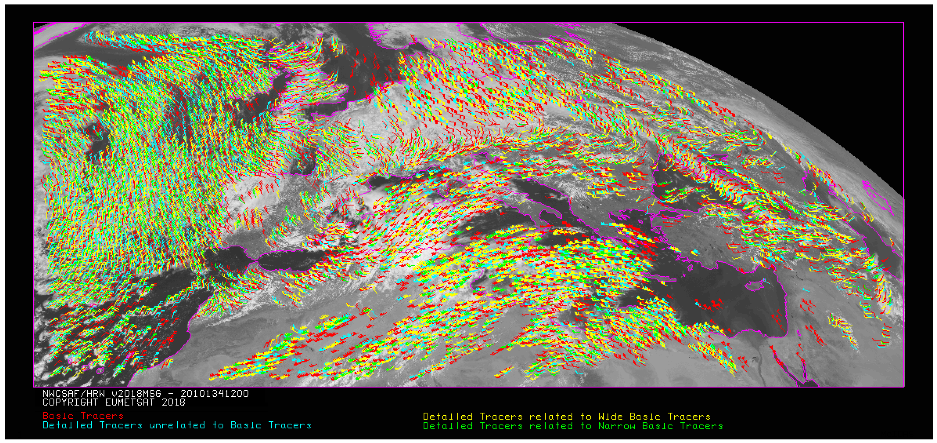
2.2.4. Detailed Tracers in the Two-Scale Procedure

The ‘basic scale’ in the ‘two-scale procedure’ works in a similar way than the procedure here described for the ‘single-scale procedure’, while additionally defining starting locations for the ‘detailed scale’, when one of following conditions are met:
  • No ‘Basic tracer’ has been found, but at the ‘tracer candidate’ the following condition occurs: CENT_97% > 102 (in visible cases) or CENT_03% < 204 (in the other cases). A ‘Detailed tracer unrelated to a Basic tracer’ is so defined, with less demanding brightness thresholds.
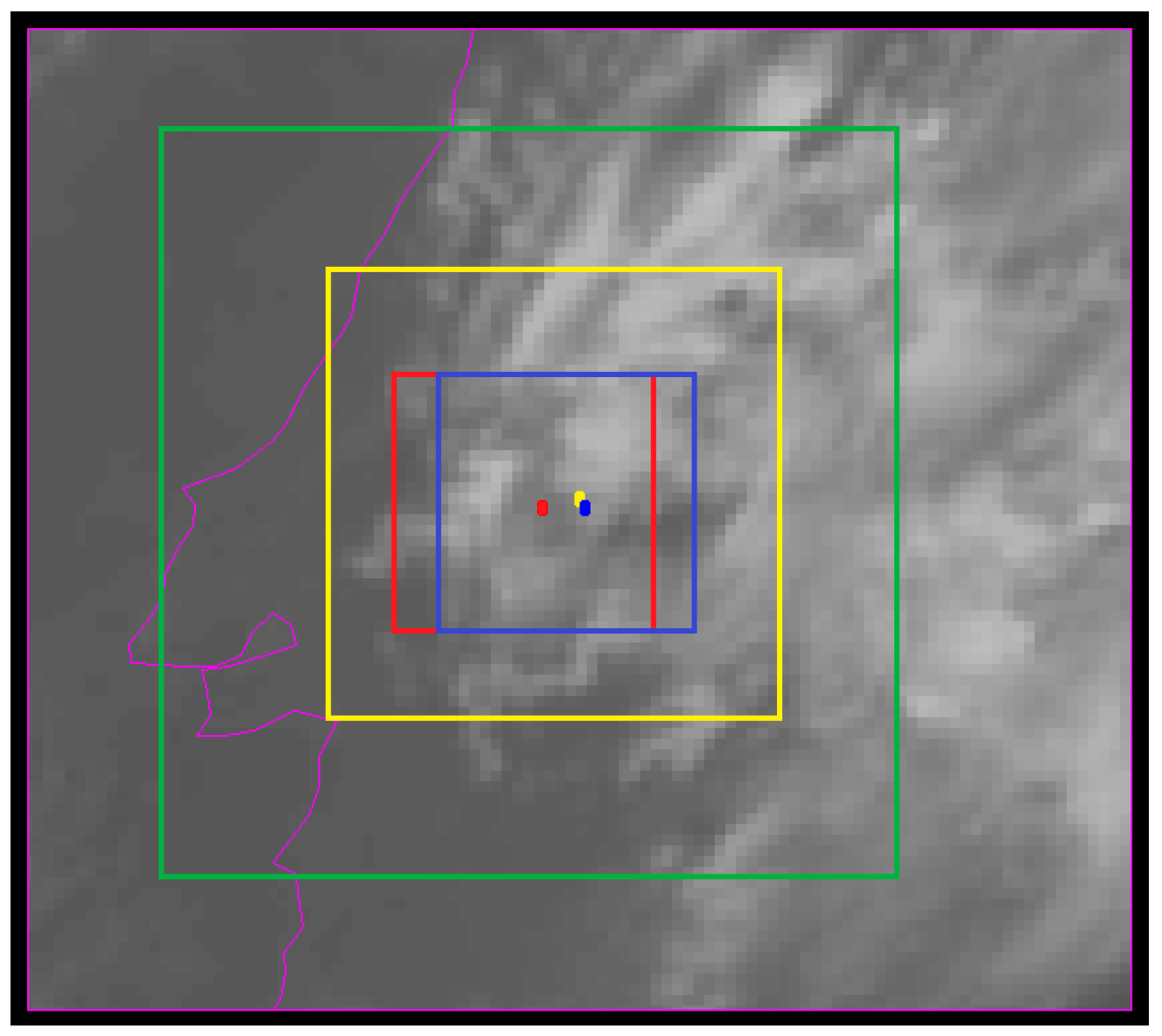
  • A ‘Wide basic tracer’ has been found, in which CLASS_2 values appear in both first and last row or column of the ‘4 × 4 big pixel matrix’, in the ‘Big pixel brightness variability test’. In this case, four starting locations are defined for the ‘Detailed scale’. Each of them is located at the corners of a ‘Detailed tracer’ whose center is the center of the ‘Basic tracer’.
  • A ‘Narrow basic tracer’ has been found, in which CLASS_2 values do not appear in both first and last row nor column of the ‘4 × 4 big pixel matrix’, in the ‘big pixel brightness variability test’. In this case, one starting location is defined for the ‘Detailed scale’, whose center is defined by the weighted location of the ‘big pixels’ in the ‘4 × 4 big pixel matrix’.
Examples of AMVs related to different types of tracers for MSG satellite series, considering the tracer method and the tracer type, are shown in Figure 3 and Figure 4.
In Figure 3, ‘basic AMVs’ are shown related to the tracer calculation method (‘gradient method’ and ‘tracer characteristics method’).
In Figure 4, ‘basic and detailed AMVs’ are shown related to the tracer type (‘basic tracers’, ‘detailed tracers unrelated to basic tracers’, ‘detailed tracers related to wide basic tracers’, and ‘detailed tracers related to narrow basic tracers’).
In Figure 5, an example of valid ‘basic AMVs’ related to the satellite channel they have been calculated with is shown.

2.3. Tracer Tracking

The tracking process looks for the location of a tracer computed in an initial image, inside a portion of a later image (‘tracking area’). The process performs a pixel by pixel comparison between the tracer brightness values and those of a square segment of the same size (‘tracking candidate’), repeatedly moving this tracking candidate throughout the tracking area. For a tracking candidate inside this tracking area, the algorithm used for the tracking is one of the well-known methods:
  • Euclidean distance, in which the sum
    LP = ΣΣ(Tij − Sij)2
    is calculated. Tij and Sij correspond to the brightness values for the tracer and the tracking candidate pixels at corresponding locations. The best tracking locations are defined through the minimum values of the sum LP. This method is for example also used by NOAA operational AMV algorithm, as defined in [7].
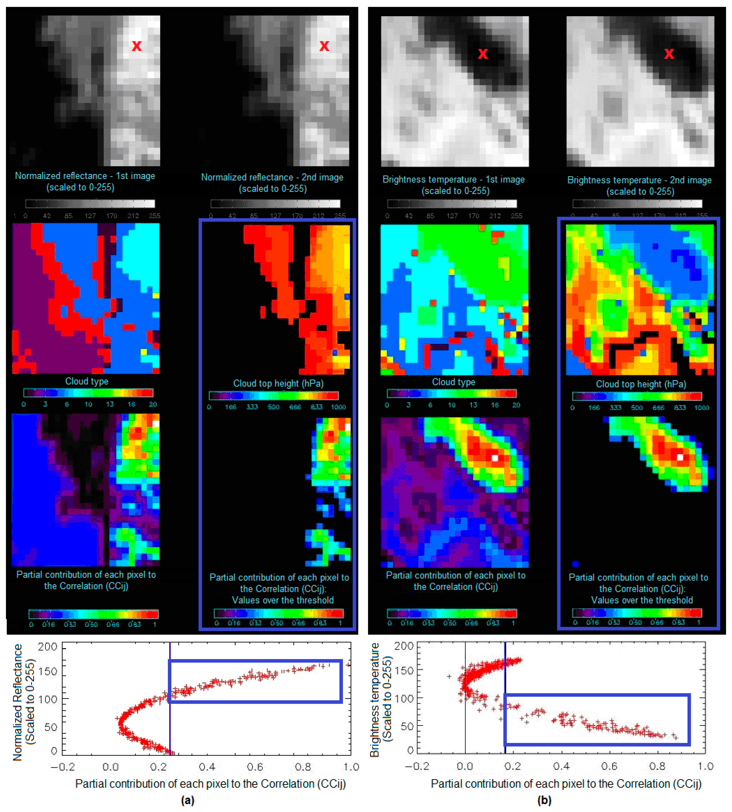
  • Cross correlation, in which the normalized correlation value
    CC = COVT,S/(σT·σS)
    is calculated (default option for the processing). T and S correspond to the brightness values for the tracer and the tracking candidate pixels; COVT,S is the covariance of these variables, and σTS is the standard deviation of the brightness values for the tracer and the tracking candidate. The best tracking locations are defined through the maximum values of the correlation CC. This method is for example also used by EUMETSAT, JMA, KMA, and CPTEC/INPE operational AMV algorithms, as defined in [7].
The center of the tracking area can preliminarily be defined through a wind guess obtained from the NWP forecast of the rectangular wind components, interpolated to the tracer location and level. This permits to reduce the tracking area size and the running time of HRW product.
However, HRW product has been optimized not to use this wind guess as default option, so reducing the dependence of the calculated AMVs from any NWP model used (although the running time is two to three times longer).
The impact of using or not using the wind guess for the definition of the tracking area is shown in Figure 6.
The line and column size in pixels of the tracking area is calculated so that it is able to detect displacements of the tracer of at least 272 km/h in any direction, when the wind guess is not used in the definition of the tracking area. This parameter is configurable.
When the wind guess is used, the parameter is to be understood as the difference in speed with respect to that of the NWP wind guess that HRW product is at least able to detect.
To avoid the computation of the Euclidean distance (LP) or the cross correlation (CC) in all locations of the tracking area, a gradual approach is performed in four iterations, based on the idea that both Euclidean distance and cross correlation change slowly, such as shown by Xu & Zhang [8].
In a first iteration, a pixel computation GAP of 8 pixels is applied: LP or CC values are evaluated only at (1,1), (1,9), …, (9,1), (9,9), … pixel locations inside the tracking area in the first iteration. The four locations with the best values of LP or CC are retained for the following iteration. In the second, third and fourth iterations, LP or CC are only evaluated if possible at four locations around each one of the four best locations retained in the previous iteration, defined by (imax ± GAP, jmax ± GAP), for which GAP reduces to a half in each one of the iterations until having the value of 1.
After all four iterations, the three tracking centers with the best Euclidean distance or cross correlation values are retained. With cross correlation, it is also requested that the best correlation value is at least greater than 80% (50% for GOES-N satellites).
Finally, in the default configuration, the line/column and latitude/longitude location of the three best tracking centers is refined through second order interpolation with ‘subpixel tracking’ process. Here, considering a tracking case with cross correlation, and being POSINT and POSREAL the line/column location of the tracking center before and after this subpixel tracking, and CC−1, CC+1, CC the cross correlation values one position up/left from, down/right from, and at the tracking center:
POSREAL = POSINT + (CC−1 − CC+1)/(2·(CC−1 + CC+1 − 2CC))

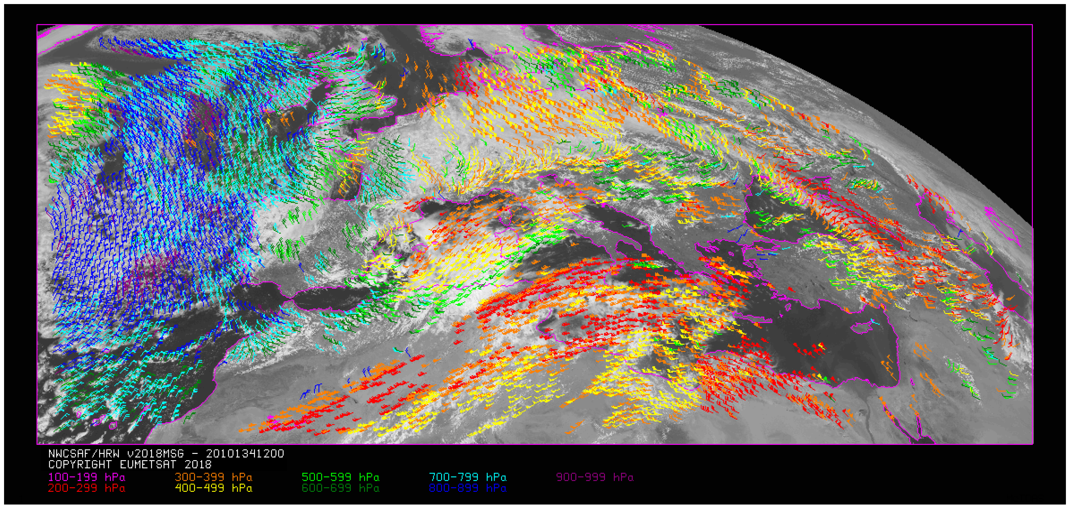
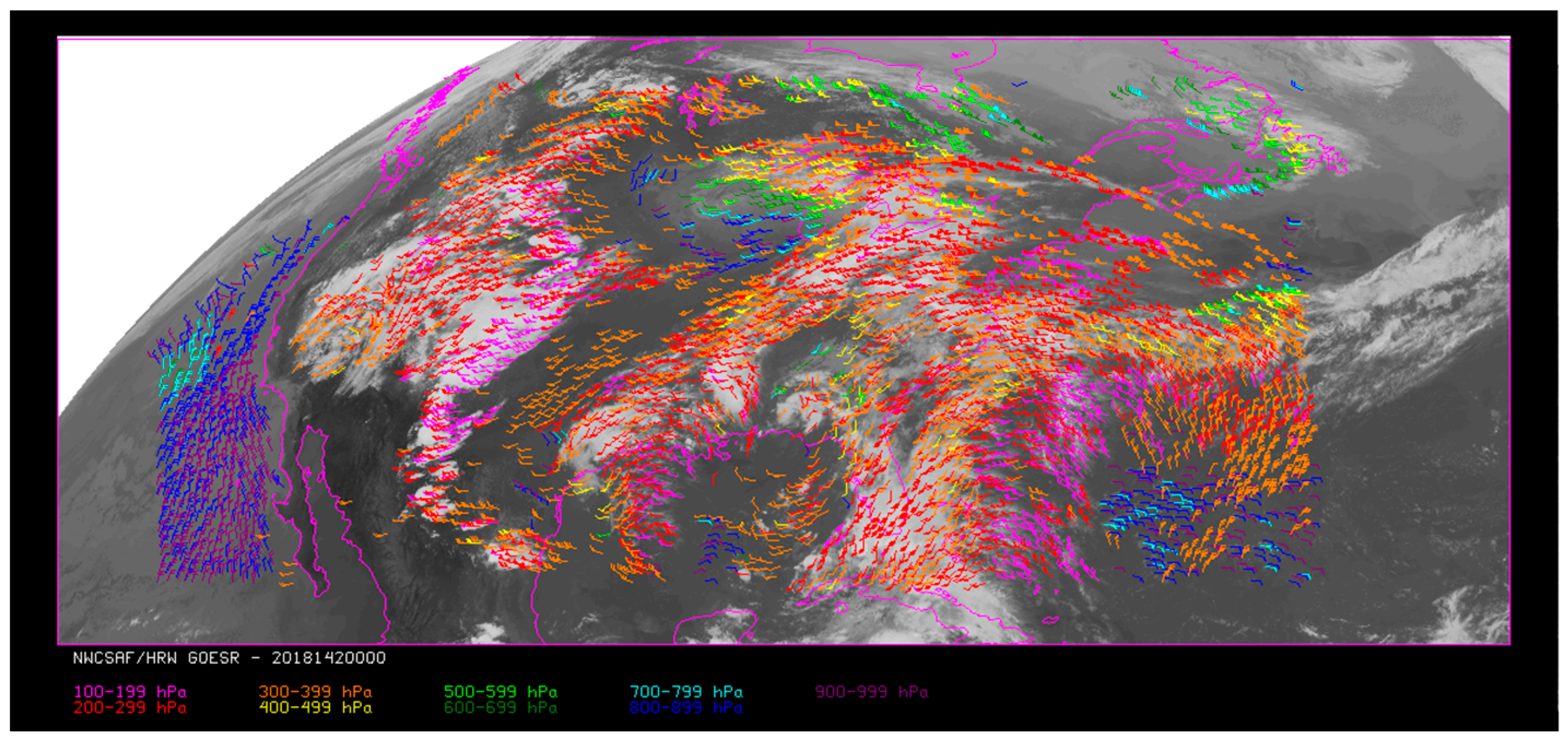
2.4. Height Assignment

2.4.1. EBBT (Effective Blackbody Brightness Temperature) Height Assignment

EBBT (effective blackbody brightness temperature) height assignment was the first option implemented in HRW product. Although not used anymore in the default configuration, it is still available in the HRW code.
The method is still used by other AMV operational algorithms partially or with variations (with the main exception of JMA, as defined in [7]). However, in general in the latest years, it is being replaced by other more sophisticated methods in all AMV processing centers.
The height assignment is based on the brightness temperature of the tracer pixels for the infrared and water vapor channels. MSG/IR108, GOES-N/IR107, Himawari-8/9 or GOES-R/IR112 brightness temperatures are used for the visible channels. With this:
  • A cloud top temperature is computed through the coldest class of the brightness temperature histogram with at least 3 pixels, after histogram smoothing.
  • A cloud representative temperature is computed with TC + 1.2σC (visible cases), and TC (other cases), where TC is the mean value and σC the standard deviation of the brightness temperature.
A conversion of these temperature values to pressure values (cloud top pressure and cloud representative pressure) is then done through interpolation inside the nearest NWP temperature forecast profile.
If NWC/GEO-CT Cloud Type product output is available, it is read to define the AMV cloud type, and which of the calculated pressure values is used as AMV pressure.
Some tracers are also eliminated depending on the AMV cloud type value and the satellite channel with which they have been calculated. These cases are identified as empty cells in Table 1, and are related to tracers in visible and infrared channels with less than a 2.5% of cloudy pixels, fractional clouds, and cloud types for which the validation statistics are significantly worse. In the rest of cases, the AMV cloud type and the AMV pressure are also defined such as shown in Table 1.

2.4.2. CCC (Cross Correlation Contribution) Height Assignment—Cloudy Cases

CCC (cross correlation contribution) method height assignment is used as default option in HRW product. This method was developed by Borde & Oyama [9], and is also used by several other AMV operational algorithms (EUMETSAT and KMA, as defined in [7]).
It requires the use of cross correlation as tracking method, and the calculation of NWC/GEO-CT cloud type and CTTH cloud top temperature and pressure outputs for the image in which tracers are tracked, before the running of HRW product. If these outputs are not available, HRW product skips this method and uses the AMV pressure and AMV temperature values provided by EBBT height assignment method.
In case the wind guess was used for the definition of the tracking area, the AMV pressure and AMV temperature values calculated by CCC height assignment method replace the values calculated previously by EBBT height assignment method.
CCC method has the advantage of including in the height assignment all procedures included in NWC/GEO-cloud products for the identification of clouds and the calculation of the cloud top pressure [10], and which are common methods used by other AMV producers, including:
  • Opaque cloud top pressure retrieval considering infrared window channels, with simulation of radiances with RTTOV radiative transfer model, and option for thermal inversion processing.
  • Semitransparent cloud top pressure retrieval with infrared window/water vapor intercept method and radiance ratioing method, considering water vapor and carbon dioxide channels.
More information about how NWC/GEO-Cloud products evaluate for the different satellites and in comparison with other available cloud algorithms can be found in Sèze et al. [11]; Hamann et al. [12]; and Choi et al. [13].
CCC method defines the AMV pressure and the AMV temperature taking into account only the pressure and temperature of the pixels contributing most to the cross correlation between the tracer in the initial image and the tracking center in the final image.
For this, the partial contribution of each pixel to the correlation (CCij) is used. It is defined by the following formula, in which respectively for the tracer and the tracking center Tij/Sij are again the brightness values for each pixel, TM/SM are the mean values and σTS the standard deviations of these brightness values, and NUM is the total number of pixels inside the tracer/tracking center:
CCij = (Tij − TM)·(Sij − SM)/(NUM·σT·σS)
The graph for normalized reflectance(partial contribution to the correlation) for the visible channels, or the graph for brightness temperature(partial contribution to the correlation) for the infrared/water vapor channels has, in general, the shape of the letter ‘C’, as shown by the lower graphs in Figure 7. The left one corresponds to a MSG/VIS08 case, and the right one to a MSG/IR108 case. In this letter ‘C’, the largest partial contribution to the correlation is given by the brightest and darkest pixels (for the visible channels), and by the warmest and coldest pixels (for the infrared/water vapor channels).
The AMV pressure and AMV temperature are calculated considering only the pixels whose partial contribution to the correlation is higher than a CCC calculation threshold inside the bright branch of the normalized reflectance(partial contribution to the correlation) graph in the visible cases. In the infrared and water vapor cloudy cases, it considers only the pixels whose partial contribution to the correlation is higher than the CCC calculation threshold inside the cold branch of the brightness temperature(partial contribution to the correlation) graph. The CCC calculation threshold is defined as the mean partial contribution to correlation, or zero if so no pixels are kept.
With all this, the AMV pressure (Pccc) and AMV temperature (TCCC) are calculated considering the partial contribution to the correlation (CCij), and the CTTH cloud top pressure (CTPij) and cloud top temperature (CTTij) outputs for the pixels defined before inside the ‘tracking center’, with the formula
PCCC = ΣΣ(CCij·CTPij)/ΣΣCCij
TCCC = ΣΣ(CCij·CTTij)/ΣΣCCij
The procedure is repeated for the three tracking centers defined for each tracer. If the ‘parallax correction’ is considered later in Section 2.5 for the position of the tracer/tracking center, a similar calculation is done for the AMV height (HCCC), considering the cloud top height (CTHij) and the equivalent formula
HCCC = ΣΣ(CCij·CTHij)/ΣΣCCij
The AMV cloud type is calculated as the one with the highest sum of partial contributions to the correlation. The AMV pressure error (ΔPCCC) is finally calculated with the formula
ΔPCCC = ((ΣΣ(CCij·CTPij2))/ΣΣCCij − PCCC2)1/2
which can be useful as a quality control parameter for the filtering of AMVs and trajectories. Here, a maximum AMV pressure error is defined with a configurable parameter (with a default value of 150 hPa).
Images in Figure 7 show in detail two examples of the running of CCC method (as already said, for a MSG/VIS08 AMV on the left side, and a MSG/IR108 AMV on the right side).
In the first row of the images, the ‘image matrices’ for the tracer pixels in the initial image, and for its tracking center pixels in the later image are shown. Visually comparing the images, it is clear that the same feature is being observed in both cases, in spite of the evolution shown in a period of 15 min.
In the second row, the NWC/GEO-CT cloud type and CTTH cloud top pressure related to the tracking center pixels are shown. In the third row, the partial contributions to the correlation for the tracking center pixels are shown: on the left considering all pixels and on the right only those pixels defined as valid by the CCC calculation threshold (which in these cases is the mean contribution to the correlation).
As already explained, the last row of the images shows respectively the normalized reflectance(partial contribution to the correlation) graph and the brightness temperature(partial contribution to the correlation) graph for these cases, with the CCC calculation threshold defined by the method as a vertical blue line. Only those pixels having a value inside the blue boxes of these graphs are used in the calculations of PCCC and ΔPCCC.
In the MSG/VIS08 example on the left, these pixels correspond to the very low and low cloud in the right part of the tracking center, defining values of PCCC = 834 hPa and ΔPCCC = 27 hPa. In the MSG/IR108 case on the right, these pixels correspond to the high cloud in the upper right corner of the tracking center, defining values of PCCC = 286 hPa and ΔPCCC = 24 hPa.
With the default configuration of HRW product, the displacement of the AMV between the tracer and the tracking center locations is not considered between the centers of these tracer and tracking center, but between the weighted locations defined with similar formulae (where Xij and Yij correspond to the line and column position of each pixel inside the tracer and tracking center)
XCCC = ΣΣ(CCij·Xij)/ΣΣCCij
YCCC = ΣΣ(CCij·Yij)/ΣΣCCij
The weighted locations relate the displacement of the AMVs and Trajectories to the displacement of the part of the tracer with the largest contribution to the cross correlation. These weighted locations are identified in Figure 7 as red crosses.
When trajectories are calculated, tracking consecutively during several images the same tracer, the calculation of these weighted locations occurs only for the first AMV in the trajectory, and keeps the same value during all the time the trajectory is alive. This way, spatial discontinuities in the trajectories are avoided.

2.4.3. CCC (Cross Correlation Contribution) Height Assignment—Cloudy Cases with Microphysics

CCC method height assignment offers a direct correspondence between the pressure levels defined for HRW cloudy AMVs and trajectories, and those given to the cloud tops by NWC/GEO-CTTH product, so avoiding any possible incongruence between both products. It also defines a clear correspondence between the elements considered for the AMV pressure calculations and the real features observed in the satellite images.
Taking this into account, several studies have suggested that AMVs are better related to a pressure level different from the cloud top: Lean et al. [14]; Hernández-Carrascal & Bormann [15]; Salonen & Bormann [16].
An empirical relationship has been found in HRW product for the difference between the AMV pressure level calculated with CCC method and the radiosonde wind best fit pressure level on one side, and the cloud depth represented by the AMV liquid/ice water path values on the other side. Therefore, a correction of the AMV pressure can be defined with these parameters.
For this procedure, the output of the NWC/GEO-CMIC Cloud microphysics product is used, which provides the cloud phase (CPhij) for each cloud pixel, the liquid water path (LWPij) for each liquid cloud pixel and the ice water path (IWPij) for each ice cloud pixel.
The ‘AMV cloud phase’ is defined in a similar way to the one used for the ‘AMV cloud type’ in the previous section, as the phase with the highest sum of partial contributions to the correlation. It has four possible values: liquid phase, ice phase, mixed phase, undefined phase.
The AMV liquid water path (LWPCCC) is then calculated for liquid phase AMVs, and the AMV ice water path (IWPCCC) is calculated for ice phase AMVs, with similar formulae to the ones used in the previous section for the AMV pressure
LWPCCC = ΣΣ(CCij·LWPij)/ΣΣCCij
IWPCCC = ΣΣ(CCij·IWPij)/ΣΣCCij
The empirical relationship for the difference between the AMV pressure level calculated with CCC method and the radiosonde wind best fit pressure level, and the AMV ice/liquid water path, has been tuned in HRW v2018.1 product for MSG and Himawari-8/9 satellites in the regions used for the validation in Section 3.1, considering for the tuning a different period than the one used for the validation. For GOES-R, due to the similarities of its ABI imager with the AHI imager included in Himawari-8/9, the same empirical relationship has been used.
For example, for MSG satellite series, it considers 12:00 UTC Cloudy AMVs calculated with MSG-2 satellite images between July 2010 and June 2011 in the European and Mediterranean region. Defining separate procedures for ice and liquid cloud visible AMVs, for ice and liquid cloud infrared AMVs, and for ice and liquid cloud water vapor AMVs, Figure 8 is obtained.
The empirical relationship is used to define a microphysics correction of the AMV pressure (for MSG satellite series shown in Table 2). Equivalent procedures are defined for Himawari-8/9 and GOES-R satellite series; for more information on them, the “Algorithm Theoretical Basis Document for the Wind product processor of the NWC/GEO” [17] is to be checked.
In this microphysics correction, a double linear/constant regression works better than a simple linear regression in all possible cases. The correction locates in general the AMVs in a level nearer to the ground, with the main exception of AMVs with small ice/liquid water path values.
A control is later defined through the Orographic flag to avoid that AMVs could be located at a level below the ground after the correction. Verifying the AMV statistics for the validation periods defined in Section 3.1, the microphysics correction causes in general a reduction in all validation parameters (defined in Appendix A), which is largest for the normalized bias (NBIAS).
CCC method with Microphysics correction height assignment is implemented as default option for MSG, Himawari-8/9 and GOES-R satellites series. It cannot be used with GOES-N because no NWC/GEO-CMIC product is available for this satellite series. With this, it is necessary to run all NWC/GEO-Cloud products (CMA, CT, CTTH, CMIC) before HRW product, so that all this process can be activated. If CMIC product output is not available but the other ones are, the HRW product runs a CCC method without microphysics correction height assignment.
An example of AMVs for MSG is shown in Figure 9, related to the option used for each AMV by CCC method height assignment (CCC method with/without microphysics correction, using the low/high CCC method calculation threshold) and the AMV phase (ice cloud AMV, liquid cloud AMV, mixed/undefined cloud AMV, clear air AMV).
Another example of AMVs is also shown in Figure 10, related to the AMV pressure correction defined by CCC method with microphysics correction, for the AMVs for which this height assignment method was used.

2.4.4. CCC (Cross Correlation Contribution) Height Assignment—Clear Air Cases

A ‘water vapor clear air AMV’ is defined as a water vapor AMV for which the sum of partial contributions to the correlation is larger for the group of clear air pixels than for the group of cloudy pixels, considering all pixels inside the tracking center for which the partial contribution to the correlation is positive. An adaptation of CCC method is implemented in HRW product for use with water vapor clear air AMVs, because logically NWC/GEO-CTTH cloud top pressure does not provide any values for clear air pixels.
The AMV cloud type and the AMV temperature are calculated in a way similar to the one described in Section 2.4.2 for the water vapor cloudy AMVs, although now the brightness temperature for each pixel (BTij) from the corresponding satellite image is used instead of the NWC/GEO-CTTH cloud top temperature for the processing. An AMV temperature error (ΔTCCC) is calculated with a formula similar to the one used for the AMV pressure error
ΔTCCC = ((ΣΣ(CCij·BTij2))/ΣΣCCij − TCCC2)1/2
Three different temperature values are then defined by the following formulae: TCCC + ΔTCCC, TCCC, TCCC − ΔTCCC. For each one of these values a temperature to pressure conversion is done through interpolation inside the nearest NWP temperature forecast profile, providing three pressure values: PCCC (related to TCCC), PCCCMAX (related to TCCC + ΔTCCC), and PCCCMIN (related to TCCC − ΔTCCC). PCCC is then defined as the AMV pressure for the clear air AMVs. The AMV pressure error for the clear air AMVs is defined as: ΔPCCC = |PCCCMAX − PCCCMIN|/2.

2.5. Wind Calculation

Once the latitude and longitude are defined for a tracer in the initial image (considering the weighted location inside the tracer defined by CCC method in the default configuration), and for the three tracking centers in the later image (considering the non-integer displacement of the tracer inside the tracking area with subpixel tracking in the default configuration), the wind components related to that displacement are calculated.
However, in HRW v2018.1 product, a ‘parallax correction’ of the latitude and longitude values of the tracer and tracking center is first implemented in the default configuration. This parallax correction corrects the horizontal deviation in their apparent positions due to their height over the Earth surface. This parallax correction takes into account the AMV height (HCCC) calculated with CCC method for cloudy AMVs, or the geopotential for the AMV pressure defined by the NWP geopotential field in other cases.
The general effect of this parallax correction is the relocation of the AMV to a position slightly nearer to the subsatellite point and a very slight reduction in the AMV and trajectory speeds, more significant when at higher levels of the atmosphere or nearer to the edge of the Earth disk.
The calculation of the wind components considers the displacement along the corresponding great circle with the ‘haversine formula’. The haversine formula calculates the wind speed and the bearing angle of the great circle between the tracer location and the tracking center location, using as input the corresponding longitude and latitude values, and the time difference between the scanning time of the pixel defining the tracer location in the initial image and the tracking center location in the later image. The west-to-east and south-to-north wind components in m/s, are then calculated with these wind speed and bearing angle values.

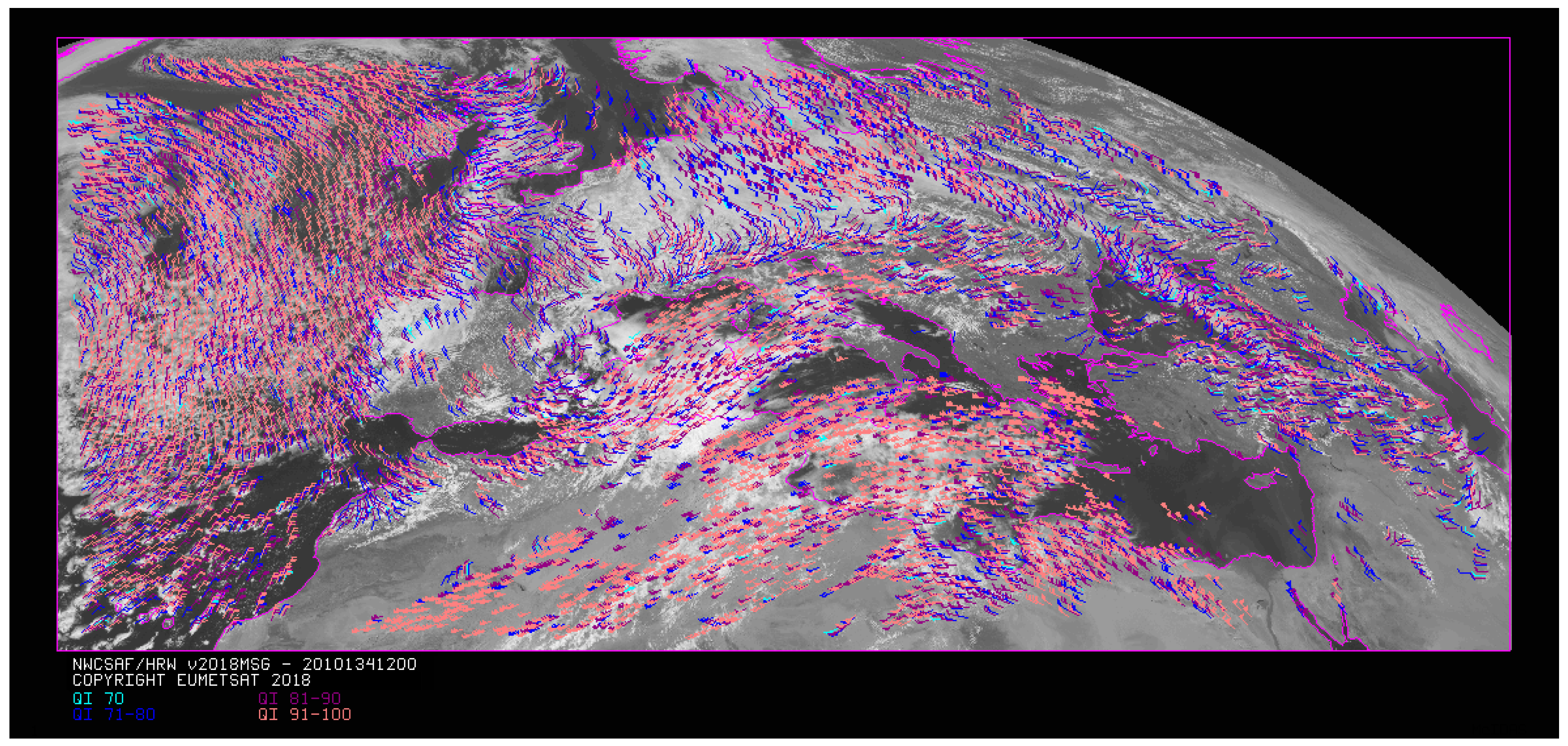
2.6. Quality Control

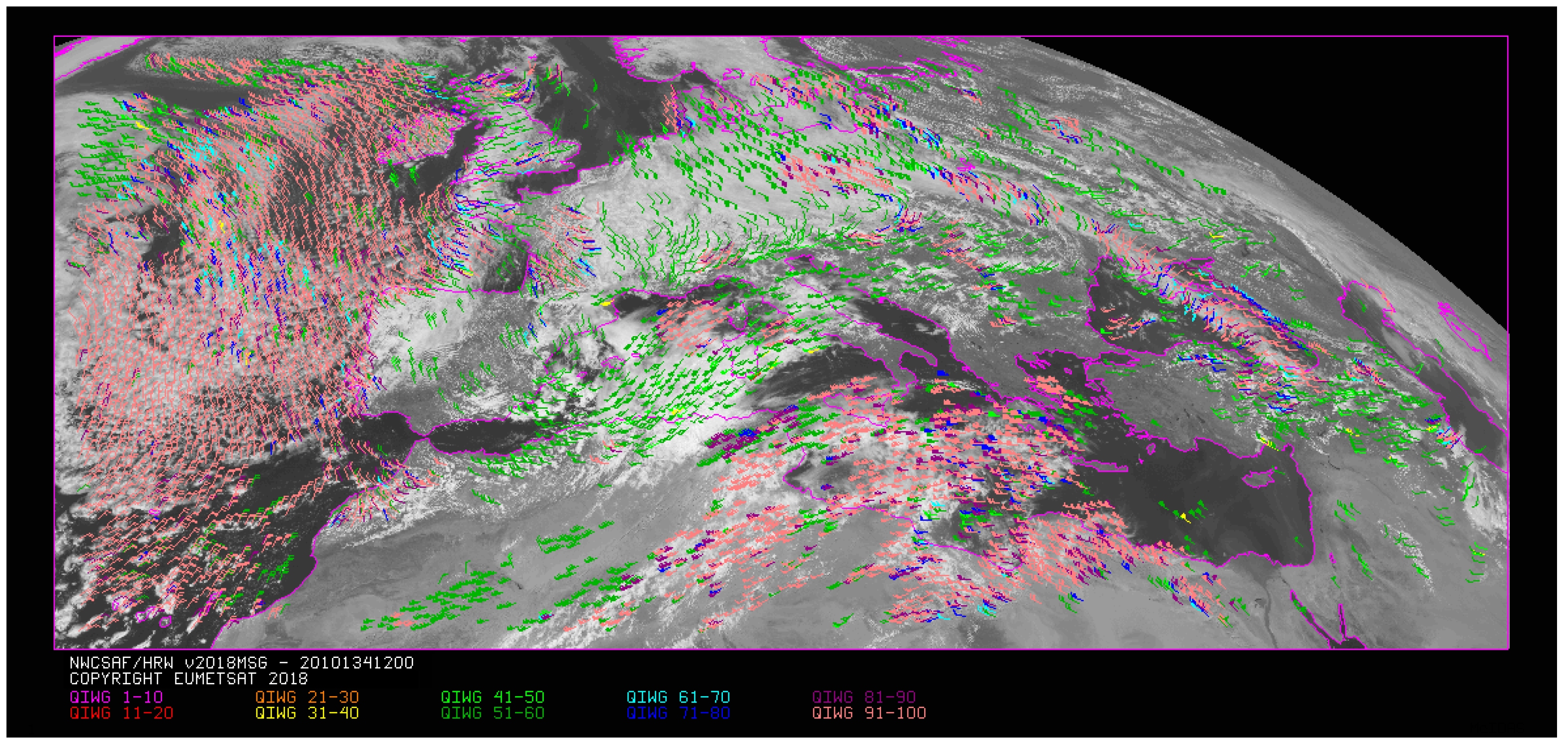
2.6.1. Quality Indicator

The quality indicator method, developed by Holmlund [18] and implemented (although with variations) by all AMV operational algorithm described in [7], is used in HRW product for the quality control. This method assigns quantitative dimensionless quality flags to all AMVs and trajectories, ranging from 0% to 100%: ‘quality indicators’ (QIs).
It is based on normalized functions, related to the expected change of the AMVs considering temporal vector consistency (comparison to a previous AMV in the previous image at the same location and level), spatial vector consistency (comparison to a neighbor AMV in the current image at the same location and level), and vector consistency relative to a background (NWP wind forecast at the same location and level).
For the two-scale procedure, an additional interscale spatial consistency is computed for detailed AMVs derived from a basic scale tracer (comparing to the corresponding basic scale AMV).
The different individual quality indicators are given by the following formulae, in which SPEED is the average wind speed for the evaluated AMV and the reference wind, and DIF is the absolute change in the module of the vector difference. SPEED and DIF are defined in m/s units.
QF = 100·(1 − (tanh(DIF/(max(0.4·SPEED, 0.01))+1))2)
(in the forecast vector consistency test)
QIi = 100·(1 − (tanh(DIF/(max(0.2·SPEED, 0.01))+1))3)
(in the other consistency tests)
The procedure is repeated for three neighbor AMVs in the spatial consistency, and three previous AMVs in the temporal consistency. The contribution from each one of these reference AMVs to the value of the spatial or temporal consistency depends on a distance factor to the evaluated AMV.
The ‘distance factor’ is given by the following formulae, in which SPEED/DIR/LAT are the speed in m/s units, the direction in ° units, and the latitude in rad units of the evaluated AMV, LATDIF/LONDIF are the latitude and longitude difference with respect to the reference AMV in rad units, and ER is the Earth radius in km units:
alpha = 200 + 3.5·SPEED
gamma = ER·(LATDIF2 + LONDIF2)1/2·cos(270 − DIR − atan(cos(LAT)+LATDIF/LONDIF))
delta = ER·(LATDIF2 + LONDIF2)1/2·sin(270 − DIR − atan(cos(LAT)+LATDIF/LONDIF))
factor = (gamma/alpha)2 + (delta/alpha)2
Only reference AMVs with a distance factor smaller than 1, a pressure difference smaller than 25 hPa and a latitude and longitude difference smaller than 1.35° are considered valid here. The three reference AMVs with the smallest distance factor are considered for the quality control.
The weighted sum of these consistency tests provides two overall values: the ‘quality indicator with forecast’ and the ‘quality indicator without forecast’. The weight of the consistency tests in the overall quality indicators are: 3 for the temporal and spatial vector consistency tests, and 1 or 0 for the forecast vector consistency test. The value 1 provides the quality indicator with forecast and the value 0 provides the quality indicator without forecast. Two corrections are nevertheless applied in the overall quality indicators before using them:
  • One correction reduces the quality indicators of AMVs with a speed lower than 2.5 m/s. It is a multiplying factor defined by the following formula, in which SPEED is the speed of the evaluated AMV in m/s and SPEED_THR = 2.5 m/s:
    Fs = SPEED/SPEED_THR
  • The other correction has the name of ‘Image correlation test’ and affects visible and infrared AMVs with a pressure higher than 500 hPa. It is a multiplying factor defined by the following formula, in which CORR(IR,WV) is the correlation of IR108/WV62 images for MSG satellites, the correlation of IR107/WV65 for GOES-N satellites, or the correlation of IR112/WV62 images for Himawari-8/9 of GOES-R satellites, at the location of the AMV tracking center:
    Fc = 1 − (tanh((max(0, CORR(IR,WV))/0.2)))200
The overall quality indicator with forecast or quality indicator without forecast are used for the filtering of the AMV and trajectory data, before writing them in the output files. The first one is used as default option. The quality indicator threshold for the acceptance of an AMV or trajectory as valid has a default value of 70%, and a minimum value of 1%. An example of valid AMVs is shown in Figure 11, related to their quality indicator with forecast.
Some additional considerations on the quality control, specific for HRW product, are:
  • All calculated AMVs are considered valid for the spatial vector consistency.
  • It is frequent that a quality consistency test cannot be calculated, for example when no reference AMV was found for the comparison. The overall quality indicators will thus only include the available quality tests.
  • For the temporal consistency of successive AMVs related to the same trajectory, some limits are defined for the consistency in the speed difference (10 m/s), direction difference (20°) and pressure difference (50 hPa), with the previous AMV in the same trajectory.
  • Each one of the three AMVs calculated for each tracer has its own quality indicators, but only one of them is selected for the HRW outputs. The selected AMV is the one which is the best for the most of following criteria: interscale spatial quality test, temporal quality test, spatial quality test, forecast quality test, and correlation (this one with a triple contribution). If this is not definitive, the AMV with the best forecast quality test prevails. If this is also not definitive, the AMV with the best cross correlation prevails.

2.6.2. Common Quality Indicator without Forecast

Through the experience in the International Winds Workshops, it was clear that the configuration of the quality indicators is very different for different AMV algorithms, and so a common homogeneous use for AMVs calculated by different AMV producers was not available.
Because of this, a self-contained Fortran module defined by EUMETSAT and NOAA/NESDIS and calculating a ‘common quality indicator without forecast’, was distributed by the International Winds Working Group in May 2017, so that it would be included as such without modifications by all AMV algorithms.
The experience of use of this common quality indicator without forecast in the 2018 AMV Intercomparison Study [19] showed some skill in filtering collocated AMVs from different AMV algorithms, improving their statistical agreement.
This common quality indicator without forecast module has been implemented in HRW v2018.1 product, and the parameter is provided as an additional third quality indicator for AMVs and trajectories. An example of valid AMVs is shown in Figure 12, related to their common quality indicator without forecast.
Differences of this common quality indicator without forecast with respect to the previous quality indicators shown in Section 2.6.1 are:
  • It is only calculated for AMVs and trajectories with at least two trajectory sectors.
  • For the spatial consistency, only the closest neighbor AMV is considered. For the temporal consistency only the previous AMV related to the same trajectory is considered.
  • Four different tests are applied: direction, speed and vector difference tests for the temporal consistency, and vector difference for the spatial consistency (with a double contribution). Formulae for the calculation of these quality consistency tests are also slightly different.
  • It is not used for the filtering of AMVs and trajectories by HRW product, so all values between 1% and 100% are possible in the AMV and trajectory outputs. In the cases for which it could not be calculated, an unprocessed value is defined.

2.7. Orographic Flag

In the default configuration of HRW product, an ‘orographic flag’ based on new development is calculated for each AMV and trajectory. The orographic flag incorporates topographic information, which in combination with NWP data, detects and rejects those AMVs and trajectories affected by land influence. The reasons for this land influence may be:
  • AMVs associated to land features incorrectly detected as cloud tracers.
  • Tracers blocked or whose flow is affected by mountain ranges.
  • Tracers associated to lee wave clouds with atmospheric stability near mountain ranges.
These tracers present displacements which do not correspond with the general atmospheric flow. Because of this, the corresponding AMVs and trajectories are not considered as valid.
The procedure to calculate the orographic flag implies the reading of NWP geopotential data and two topography matrices for the defined satellite and positioning. These matrices define the 3% and 97% centiles of the topography histogram for each pixel, in which data up to 1 degree away are considered. They are called the ‘representative minimum and maximum height matrices’ for each pixel.
These matrices are then converted to ‘representative maximum and minimum surface pressure matrices’ with NWP geopotential data. To do this, the height matrices are converted to geopotential values, and the geopotentials are then inversely interpolated to NWP pressure to define the representative maximum and minimum surface pressure values for each pixel (PMIN, PMAX). These values represent the highest and lowest representative surface pressure values in locations up to one degree away of each pixel of the image.
After this, the orographic flag is calculated. Possible values are:
  • Orog.flag = 0. (The orographic flag could not be calculated).
  • Orog.flag = 1: PAMV > PMIN. AMV wrongly located below the lowest representative pressure level, mainly due to microphysics corrections in the AMV pressure value.
  • Orog.flag = 2: PAMV > PMAX + (PMIN − PMAX)/2. Very important orographic influence at the AMV position.
  • Orog.flag = 3: PAMV > PMAX − 25 hPa. Important orographic influence at the AMV position.
  • Orog.flag = 4: Very important orographic influence was found at a previous position of the AMV (for which orographic flag = 2 or 4).
  • Orog.flag = 5: Important orographic influence was found at a previous position of the AMV (for which orographic flag = 3 or 5)
  • Orog.flag = 6: No orographic influence is found in any current or previous position of the AMV.
In the default configuration, all AMVs and trajectories with any orographic influence (i.e., with orographic flag = 1 to 5) are eliminated from the HRW output files.

2.8. Final Control Check and Output Data Filtering

After the quality control, sometimes an AMV is detected to have a direction or velocity completely different to the ones in its immediate vicinity, without clearly justifying the reason for such changes in direction or velocity. They can be considered as errors.
To remove these errors, a function based on new development and called ‘final control check’ is run by the HRW product. This function calculates the velocity and direction histograms for all valid AMVs calculated with the same satellite channel in small areas inside the processing region (square boxes of 5 × 5 degrees of latitude and longitude).
When any of the columns of the velocity or direction histograms has only one element, the AMV is excluded. The procedure considers that the lack in the same area of another AMV with similar velocities or directions is enough to consider that particular AMV as an error.
Several output data filterings are additionally considered in this step, which depend on the value of several configurable parameters.
These configurable parameters are:
  • AMV BANDS, which defines the channels for which AMVs and trajectories are calculated.
  • CLEAR AIR AMVS, which defines if clear air water vapor AMVs are calculated. They are included in the default option.
  • QI THRESHOLD, which defines the quality indicator threshold for the AMVs and trajectories in the output files. As already said, the quality indicator with forecast or the quality indicator without forecast can be used for this. The first option is used as default one, with a threshold of 70%.
  • MAXIMUM PRESSURE ERROR, which defines the maximum AMV pressure error in the output AMVs and Trajectories, with CCC method height assignment. Default value: 150 hPa.
  • MIN CORRELATION, which defines the minimum correlation in the output AMVs and trajectories, when cross correlation tracking is used. Default value: 80% (50% for GOES-N).
  • FINAL FILTERING, which defines several filterings in the output AMVs and trajectories, depending on its value, on the AMV pressure filtering defined in Table 3, on the AMV cloud type defined in Table 1, and on the spatial vector consistency test.

2.9. Autovalidation Process of NWC/GEO-HRW Product

Considering requests from NWCSAF users, HRW v2018.1 product offers the option to calculate validation statistics for its AMVs with the product itself (using as reference NWP analysis or forecast components of the wind, interpolated to the AMV final location and level). The validation statistics can be calculated using NWP forecast winds in real time processes, and using NWP forecast or analysis winds in reprocessing tasks. The validation statistics are calculated at the end of the process of each HRW run for each satellite slot.
This process is implemented in the default configuration for validation against NWP forecast winds, with statistics for all layers together and for the different satellite channels and AMV types (basic AMVs and detailed AMVs, cloudy AMVs and clear air AMVs) separately. Additional options exist for other separate or joint processing of layers, channels and AMV types.
The parameters calculated in this autovalidation are exactly those defined later in Appendix A for the validation of HRW product: number of collocations (NC), mean reference wind speed (SPD), normalized bias (NBIAS), normalized mean vector difference (NMVD), and normalized root mean square vector difference (NRMSVD). They are written in the running log of HRW product, and in a specific file defined for that purpose. They can be used by the NWCSAF user as an additional tool for the quality monitoring of the HRW outputs.
The NWP reference wind which validates each AMV, the vector difference with the NWP reference wind, and the NWP reference wind at the AMV best fit pressure level (all of them defined by their speed and direction, and the last one also by its pressure value), are also calculated and added to the HRW output files by this autovalidation process.
The first one allows NWCSAF users a quick recalculation of the HRW validation parameters for different sampling and filtering options of the data, including for example monthly or yearly totalizations. The second one can be used for example for nowcasting tasks, so that the users are able to detect cases for which the AMV is very different to the NWP forecast wind, and may be aware if a warning is needed in some case due to strong winds unforeseen by the NWP forecast. Finally, the third one can be used for example for verification tasks of the AMV height assignment, to know in which cases there is more or less agreement between the AMV pressure defined for the AMVs and trajectories, and the one suggested by the NWP model reference.
The calculation of the NWP reference wind at the AMV best fit pressure level consists of two steps: first, the NWP level with the smallest vector difference between the observation and the NWP wind is found. Then, the minimum is calculated by using a parabolic fit of the vector difference for this NWP level and the two neighboring levels.
The calculation is based on the procedure defined by Salonen et al. [20], and is only defined at some specific circumstances, to avoid broad best fit pressure level values which are not very meaningful: the minimum vector difference between the observed and the NWP reference wind at best fit pressure level has to be less than 4 m/s, and the vector difference has to be greater than the minimum difference plus 2 m/s outside a band that encompasses the best fit pressure level ±100 hPa. This way, only around a 40–50% of the AMVs have a defined value for the NWP reference wind at the best fit pressure level.

2.10. Dependence from NWP Model Input Data

A description is shown here about the dependences of NWC/GEO-HRW on NWP model data.
On one side, the specific dependence of NWC/GEO-HRW on NWP model data is small. In its default configuration, the height assignment of water vapor clear air AMVs depends on the NWP forecasts for the temperature vertical profile as defined in Section 2.4.4, the calculation of the quality indicator with forecast depends on the NWP forecasts for the vertical wind profile as defined in Section 2.6, and the parallax correction of the AMV location defined in Section 2.5 and the orographic flag defined in Section 2.7 depend on the NWP forecasts for the geopotential vertical profile.
This way, deactivating the clear air AMVs, the parallax correction and the orographic flag, and using the quality indicators without forecast for the processing, NWC/GEO-HRW is specifically independent of NWP model data.
However, due to the use of NWC/GEO-Cloud products in the AMV and trajectory height assignment, the dependence of these products on NWP model data are extended to NWC/GEO-HRW product. Considering the default configuration with ECMWF model, the characterization of a pixel as cloudy and its cloud type in NWC/GEO-CT product depend on the NWP forecasts for the surface temperature and geopotential, the total water vapor and the temperature vertical profile. The cloud top pressure and height in NWC/GEO-CTTH product depend additionally on the NWP forecasts for the surface and tropopause pressure, the 2-m temperature, and the geopotential and relative humidity vertical profiles. Finally, NWC/GEO-CMIC cloud microphysics depends on the NWP forecasts for the total ozone. The main impacts of NWP model data on NWC/GEO-Cloud products are specifically related to:
  • The cloud detection (some clouds may not be detected and some false alarms may occur, mainly over land, if wrong NWP forecasts for surface temperature are used).
  • The cloud type (the separation between low/mid/high/very high clouds is based on thresholds related to the NWP forecasts for the temperature vertical profile, with marginal impact).
  • The cloud top height (NWP forecasts for the temperature and humidity vertical profiles are used; here the impact can be large if the NWP forecasts are wrong, for example with low level thermal inversion).
  • The liquid/ice water path (related to the NWP forecasts for total ozone, with limited impact).
More details about the dependences of the Cloud products on NWP model data can be obtained in the “Algorithm Theoretical Basis Document for the Cloud Product Processors of NWC/GEO” [10].

2.11. Outputs of NWC/GEO-HRW Product

Four different types of outputs are possible for NWC/GEO-HRW product:
  • OUTPUT FORMAT = EUM: one BUFR file using the “Heritage AMV BUFR sequence” defined by the International Winds Working Group (IWWG) more than a decade ago, which is used by most of AMV operational algorithms, permitting a common processing for all AMV datasets.
  • OUTPUT FORMAT = IWWG: one BUFR file using the “New 310,077 AMV BUFR sequence” defined in 2018 by the IWWG, which is being implemented by most of AMV operational algorithms as a substitute of the previous one. This sequence also permits a common processing for all AMV datasets with this format.
  • OUTPUT FORMAT = NWC (default option): two different BUFR files for AMVs and Trajectories, related to the ones used in all previous versions of HRW product, so permitting continuity of use throughout the different versions of HRW product.
  • OUTPUT FORMAT = NET: one NetCDF file, requested by the NWCSAF users for a common processing of all NWCSAF products.
Different outputs are obtained for each scale (basic AMVs and detailed AMVs if so configured), for each one of these formats, for each processing region, for every running slot.
More details about the contents of NWC/GEO-HRW product output files can be obtained in the “Algorithm Theoretical Basis Document for the Wind product processor of NWC/GEO” [17].

3. Results

3.1. Validation of NWC/GEO-HRW v2018.1 AMVs

The validation of the default configuration of NWC/GEO-HRW v2018.1 AMVs, considering ECMWF NWP model data with a spatial resolution of 0.5 degrees and a temporal resolution of 6 h for the AMV calculation, and radiosonde winds as reference validation winds, is shown here for MSG, Himawari-8/9, GOES-N, and GOES-R satellite series.
The validation statistics defined at the Third and Fourth International Winds Workshops [21,22], and recommended by the Coordination Group for Meteorological Satellites (CGMS) for the international comparison of satellite winds, are used here. Appendix A shows full information on these validation statistics.
The validation of NWC/GEO-HRW v2018.1 AMVs for the different satellite series is shown considering all AMVs together and in three separate layers (high: 100–400 hPa; medium: 400–700 hPa; low: 700–1000 hPa) in Table 4, Table 5, Table 6 and Table 7 in the following pages. When the tables are compared:
  • Considering the density of AMV data for the different satellites, equivalent amounts of MSG, Himawari-8/9 and GOES-R AMVs are obtained for regions of similar size. The smaller amount of GOES-N AMVs is explained by the smaller number of satellite channels used in its processing.
  • Considering the distribution of AMVs in the different layers, the proportion of AMVs for the high/medium/low layer for the different satellites series is:
    • For MSG: 52%/25%/23% (for validated AMVs) and 45%/23%/32% (for calculated AMVs).
    • For Himawari: 82%/14%/4% (for validated AMVs) and 78%/14%/8% (for calculated AMVs).
    • For GOES-N: 86%/7%/7% (for validated AMVs) and 69%/12%/19% (for calculated AMVs).
    • For GOES-R: 86%/12%/2% (for validated AMVs) and 82%/11%/7% (for calculated AMVs).
  • Here, the higher density of tracers related to low and very low clouds has a good impact in the distribution of AMVs in the different layers for MSG satellite series. This contributes to a better characterization of the wind in the different atmospheric levels.
  • For Himawari-8/9, GOES-N and GOES-R AMVs, the higher concentration of AMVs in the High layer is basically caused by the regions used for the validation (with large high altitude and desert areas, and so less frequent low clouds). Considering for example AMVs calculated in the Himawari-8 Full Disk for IR112 channel, the distribution of AMVs for the high/medium/low layer is 52%/15%/33%, more in consonance with the result for MSG satellite series.
  • Considering the different layers, the validation parameters are progressively higher for the high layer, medium layer and low layer. This is a general result of all AMV calculation algorithms.
  • Considering the different satellite channels, MVD and NRMSVD parameters seem very different with all layers together, with changes up to a 50% between the best case and the worst case for each satellite series. This is mostly caused by the different proportion of AMVs in the different layers for each channel. Inside each one of the layers, the differences are much smaller.
  • Comparing with the equivalent statistics for MSG AMVs, the validation statistics for Himawari-8/9 AMVs show better NMVD and NRMSVD values (up to a 10% smaller), due to its larger proportion of High layer AMVs. NBIAS parameter shows similar values but with an opposite sign. Considering each layer, validation parameters are similar in the high layer, while the NMVD and NRMSVD are up to a 15% worse for the medium and low layer for Himawari-8/9.
  • Comparing with the equivalent statistics for MSG AMVs, the validation statistics for GOES-N AMVs have differences up to 15%, in many cases for the better.
  • Comparing with the equivalent statistics for Himawari-8/9 AMVs, the validation statistics for GOES-R AMVs are equivalent for the high layer, and around a 15% better for the medium and low layer. Comparing with GOES-N AMVs, the validation statistics for GOES-R are similar (with differences generally smaller than a 10%), but with at least five times more AMVs.
  • Considering the ‘Product Requirement Table’ defined by EUMETSAT for the operational use of HRW product, the ‘optimal accuracy’ is reached in the high layer, and the ‘target accuracy’ is reached in the medium and low layer for the four satellite series. EUMETSAT declared HRW product operational more than 10 years ago, and with these validation results it can be considered this way for the four satellite series.
With all this, the main circumstance to be taken into account when using NWC/GEO-HRW product is the variability with time of the amount and density of AMVs and Trajectories. This is related to the presence of cloudy areas or cloudless areas with humidity patterns in the processing region.
Considering the trajectories, the limitation is also related to the persistence in time of the tracers defining the trajectories: after one hour, only about 30% to 50% of the tracers persist; after three hours, only about 5% to 15% of the tracers persist. The persistence is different in different meteorological situations, in which the temporal change of the atmospheric structures can be quicker or slower. Therefore, the density of trajectories can be very different in different parts of an image.

3.1.1. Validation for MSG Satellite Series

The validation of HRW v2018.1 AMVs for MSG satellite series in Table 4, is based on AMVs calculated during the yearly period July 2009–June 2010 at 12:00 UTC, with MSG-2 satellite images, in the region covering Europe and the Mediterranean Sea shown in Figure 13.

3.1.2. Validation for Himawari-8/9 Satellite Series

The validation of HRW v2018.1 product for Himawari-8/9 satellite series in Table 5, is based on AMVs calculated during the half-yearly period March–August 2018 at 00:00 UTC, with Himawari-8 satellite images, in the region covering China, Korea, and Japan shown in Figure 14.

3.1.3. Validation for GOES-N Satellite Series

The validation of HRW v2018.1 product for GOES-N satellite series in Table 6, is based on AMVs calculated during the yearly period July 2010–June 2011 at 05:45/11:45/17:45/23:45 UTC with GOES-13 satellite images, in the Continental United States shown in Figure 15.
These times were used because no images exist exactly at the main synoptic hours. Validation four times a day is also considered, to reduce the issue of the small number of validated visible AMVs (dawn or dusk conditions occurs at the main synoptic hours, 00:00 and 12:00 UTC, with the largest number of radiosonde observations).

3.1.4. Validation for GOES-R Satellite Series

The validation of HRW v2018.1 product for GOES-R satellite series in Table 7 is based on AMVs calculated during the half-yearly period March–August 2018 at 00:00/12:00 UTC, with GOES-16 satellite images, in a region covering the continental United States, such as shown in Figure 16. This validation considers GOES-R mode 3 scanning, with full disk images separated every 15 min.
A significant validation period was not ready for the preparation of this paper with GOES-R mode 6 scanning, with full disk images every 10 min, operational since April 2019. However, due to the similarities in the validation results for Himawari-8 (with images every 10 min) and GOES-16 (with images every 15 min), and the similarities in both imagers (AHI and ABI), the impact of the change in the GOES-R scanning mode is assumed to be not significant in the validation statistics.

3.2. AMV Intercomparison Studies with MSG and Himawari-8/9 Satellite Data

In 2014 and 2018, two AMV intercomparison studies were proposed by the International Winds Working Group (IWWG), for the comparison of different AMV algorithms across the world [19,23]. Although the studies were financed and coordinated by the NWCSAF, the analysis and research was made by scientists from SSEC/UW (the Space Science Engineering Center of University of Wisconsin-Madison), unrelated to any of the AMV algorithms involved.
Two triplets of MSG-2 IR108 full disk images for 17 September 2012, and Himawari-8 IR104 full disk images for 21 July 2016 were used in each one of these studies. All other input needed for the AMV calculation (additional satellite channels, ECMWF NWP grids, and scene and cloud products provided by EUMETSAT and NOAA) were also provided so that all inputs would be exactly the same for all AMV algorithms.
The AMV intercomparison studies analyzed the AMV algorithms for the following producers:
  • Brazil Center for Weather Forecasting and Climate Studies (CPTEC/INPE).
  • European Organization for the Exploitation of Meteorological Satellites (EUMETSAT).
  • Japan Meteorological Agency (JMA).
  • Korea Meteorological Administration (KMA).
  • National Oceanic and Atmospheric Administration (NOAA).
  • Satellite Application Facility on support to Nowcasting (NWCSAF, NWC/GEO-HRW).
  • China Meteorological Administration (CMA, only in the 2014 Intercomparison with MSG).
Considering the ‘2014 AMV intercomparison study’ with MSG satellite images [23]:
  • The tracking step of all AMV algorithms works correctly, with displacement differences which are statistically not significant.
  • Significant differences occur in the AMV outputs, when only the MSG-2 IR108 images and NWP model data are used for the height assignment. The differences are related to the way the AMV temperature is defined by each algorithm. Considering the AMV validation against radiosonde winds and the NWP background winds, NWC/GEO-HRW product shows the lowest vector RMS of 5–6 m/s.
  • Using a prescribed configuration for the AMV extraction, a smaller number of AMVs and fewer differences in the AMV validation occur for the different AMV producers.
  • Using the specific height assignment method of each AMV algorithm, the impact is positive for all AMV algorithms except for CPTEC/INPE and JMA. NWC/GEO-HRW product shows again here the lowest vector RMS of 4 m/s.
With all this, NWC/GEO-HRW product shows the best results of all AMV algorithms with MSG satellites. Its advantages with respect to other AMV algorithms are shown: a better density of AMVs with better validation results. Its applicability to operational use is also fully demonstrated.
The key for this seems to be the CCC method height assignment used by NWC/GEO-HRW and its extensive but exigent procedure for the definition of tracers. This induces a smaller number of AMV with very good statistics in similar conditions to other AMV algorithms, while in its operational conditions the number of AMVs increases significantly with still very good statistics.
Considering the ‘2018 AMV Intercomparison Study’ with Himawari-8 satellite images [19], the main goal was to verify the advantages of the calculation of AMVs with this new generation of geostationary satellites, with better spatial and temporal resolution and new spectral channels, and to extract conclusions about the best options for the calculation of AMVs taking into account the options defined by the different centers.
The following conclusions were extracted:
  • Using a prescribed configuration with the specific height assignment method of each center, the distribution of AMV pressures is very different for all centers (with only EUMETSAT and NWCSAF being similar due to the common use of CCC method), while the distribution of other parameters (speed, direction, common quality indicator) is similar for all centers.
    Considering the validation of all AMV algorithms against radiosonde winds, JMA algorithm shows the lowest vector RMS of 5 m/s, and NOAA and NWCSAF NWC/GEO-HRW algorithms are tied in second position with a vector RMS of 7 m/s.
    For collocated AMVs against NWP analysis winds, the differences between centers reduce very much, with only JMA algorithm having better values and CPTEC/INPE algorithm having worse values than all the rest (which share a vector RMS of 4 m/s). Evaluating the fitting of the AMV pressure to the best fit pressure level, JMA AMVs show additionally to be nearer to the best fit pressure level; much more than all other datasets.
  • Using the specific configuration and the specific height assignment method of each center, the distribution of AMV pressures is again very different for all centers while the distribution of other parameters is still similar. This way, it is seen that the differences in the height assignment process drive the majority of differences observed.
    Considering the validation of all AMV algorithms against radiosonde winds, JMA algorithm shows again the lowest vector RMS of 6 m/s, and NOAA and NWCSAF NWC/GEO-HRW algorithms are tied again in second position with a vector RMS of 7 m/s.
    For collocated AMVs against NWP analysis winds, the differences between centers are larger due to the specific configuration used by each center for the AMV extraction. JMA algorithm shows again the best values, and NOAA and NWC/GEO-HRW algorithms are tied again in second position. Evaluating the fitting of the AMV pressure to the best fit pressure level, JMA AMVs are again nearer to the best fit pressure level; much more than all other datasets.
  • A validation is also made collocating the AMVs from all centers with NASA and CNES CALIPSO satellite, which provides an independent measurement of cloud top heights. The evaluation is qualitative, because CALIPSO is a line-of-site measurement, with few collocations with AMVs (tens of matches only). In this validation, AMVs from all centers are in general located near the cloud base for high level and semitransparent clouds, and near the cloud top for low and medium level clouds. Curiously, the AMV pressures for the different centers in this specific case are similar, in apparent disagreement with the previous results.
With all this, the JMA AMV algorithm for Himawari-8/9 has the best overall performance related to all validation and checking elements, due to its updated height assignment procedure: ‘optimal estimation method using observed radiance and NWP vertical profile’. This is the most significant result of this study.
NWC/GEO-HRW product has the second-best results together with NOAA AMV algorithm. With this, its applicability to operational use with Himawari-8/9 satellites is also fully demonstrated.

4. Discussion

4.1. Use of NWC/GEO-HRW Product

NWC/GEO-HRW product is provided inside NWC/GEO software package, which has to be installed and run locally by the NWCSAF users in their own hardware resources, to obtain the corresponding outputs of AMVs and trajectories.
The right to use, copy or modify NWC/GEO software package is in accordance with the corresponding policy defined by EUMETSAT. In case of interest on using NWC/GEO software package and NWC/GEO-HRW product, all National Meteorological Services within EUMETSAT Member and Cooperating States are automatically considered as potential users. All other organizations may also apply to become user of NWCSAF software. This is done contacting through email at [email protected].
All applicants have become users of NWC/GEO software without restriction up to now, with institutions and researchers from all around the world (Europe, Africa, Americas, Asia, …), and all types of institutions: national meteorological services, universities, public service providers, and public and private companies.
The access to NWC/GEO software package and documentation is authorized to users through the ‘Licence Agreement’, to be signed by EUMETSAT (represented by AEMET) and the applicant user. Once the ‘Licence Agreement’ is signed, ‘Access Credentials’ to the NWCSAF Helpdesk (www.nwcsaf.org) restricted area are provided, from which the NWC/GEO software package can be downloaded. All software, libraries, and elements needed to run the software are provided this way.
Hardware resources used to run NWC/GEO v2018.1 software package are small and relatively easy to obtain. The Linux environments defined in Table 8 have been used for the development and testing. These resources are enough for the operational and near real time generation of the full set of NWC/GEO products with MSG satellites in a continental region (~2 million pixels). The generation of products in a larger area could require additional resources related to memory, disk, and/or CPU.
The correct running in other environments cannot be currently guaranteed.

4.2. Installation and Running of NWC/GEO-HRW Product

For the running of the NWC/GEO software package and NWC/GEO-HRW product, two main steps are identified. The user manually interacts with the NWC/GEO software package during the installation step, and then the NWC/GEO-HRW product execution step is manually or automatically run (in this case, monitored by a ‘Task Manager’).
The software installation step only requires the decompression of a few gzip compressed tar files, and the running of a few installation scripts.
The software execution step is the processing of satellite images from a defined satellite in a region defined by the user, with the different executables for the different requested NWC/GEO products (including NWC/GEO-HRW product).
The running of each one of these executables relies on the running of the corresponding command together with three parameters: the required image time, the region configuration file (identifying the region inside the satellite disk in which the products are calculated), and the model configuration file (identifying the specific configuration of each product for the running).
The running also depends on a satellite configuration file, which defines the conditions for the satellite used in the processing. All these configuration files are ASCII files, in which several parameters are defined and modifications can be easily performed with a text editor.
Considering this, as already said in previous sections, the default running of HRW product implies the consecutive running of all next products for the same image and region so that the amount and quality of calculated AMVs and trajectories is optimal: Cloud Mask (CMA), Cloud Type (CT), Cloud Top Temperature and Height (CTTH), Cloud Microphysics (CMIC; not available for GOES-N satellite series), and finally High Resolution Winds (HRW).
The HRW model configuration file includes a total of 61 parameters which can modify the conditions for the extraction of AMVs and trajectories.
A short description of these parameters follows:
  • Identification parameters, which define the NWC/GEO product, the satellite channels used, and the time difference between the image slots for the tracer definition and tracking.
  • Output parameters, which define the HRW product output format and content.
  • Output filtering parameters, which define options for the process (calculation or not of clear air AMVs, trajectories, and detailed AMVs and trajectories), and the different filterings used for the AMV and trajectories in the output files (based on the quality indicator threshold, AMV pressure error and correlation thresholds, solar and satellite zenith angle thresholds, and the orographic flag and final control check defined in Section 2.7 and Section 2.8).
  • Working region description parameters, which define latitude and longitude limits for the calculations.
  • Tracer parameters, which define the dimension and distance between tracers, the use of a higher density for low tracers, and the gradient threshold and contrast used by gradient method in Section 2.2.1 for the tracer search.
  • Tracking parameters, which define options for the tracking method to be used, the use of the wind guess for the definition of the tracking area, the size of this tracking area, and the use of the parallax correction described in Section 2.5 to define the AMV.
  • Validation parameters, which define if validation statistics are calculated for the AMVs, if the NWP analysis or forecast is used for these statistics, and if the vector difference between the AMV and the NWP wind and the NWP wind at the best fit pressure level are calculated.
  • NWP parameters, which define the NWP variables and levels needed for the processing, and the way these NWP variables are extracted from the corresponding grids.

4.3. Documentation of NWC/GEO-HRW Product

Full details on the installation and use of the NWC/GEO software package, High Resolution Winds (HRW), and the cloud products used by HRW (Cloud Type (CT), Cloud Top Temperature and Height (CTTH), and Cloud Microphysics (CMIC)) can be obtained from the official NWC/GEO documentation, in the NWCSAF Helpdesk (www.nwcsaf.org). The main documents for this are:
  • “User Manual for the NWC/GEO: Software Part” [24].
  • “User Manual for the Wind product processor of the NWC/GEO: Science Part” [25].
  • “Algorithm Theoretical Basis Document for the Wind product processor of NWC/GEO” [17].
  • “Scientific and Validation Report for the Wind product processor of the NWC/GEO” [26].
  • “Algorithm Theoretical Basis Document for the Cloud product processors of NWC/GEO” [10].
Additionally, since 2016, a description of all NWC/GEO algorithms, involved interfaces and data types, is provided for the NWCSAF users with the support of Doxygen in html format, from comments included within the C and Fortran code of HRW product. This way, all this information can be easily navigated with a web browser. Through this, every single step throughout all functions of HRW product has been described with detailed comments, so that any AMV developer can precisely know all the processes within the HRW algorithm code.
For any additional doubt or question on NWCSAF Consortium, and about how to get, install and run the NWC/GEO software package and the High Resolution Winds (NWC/GEO-HRW) product, the NWCSAF Helpdesk can be contacted through the email address: [email protected].

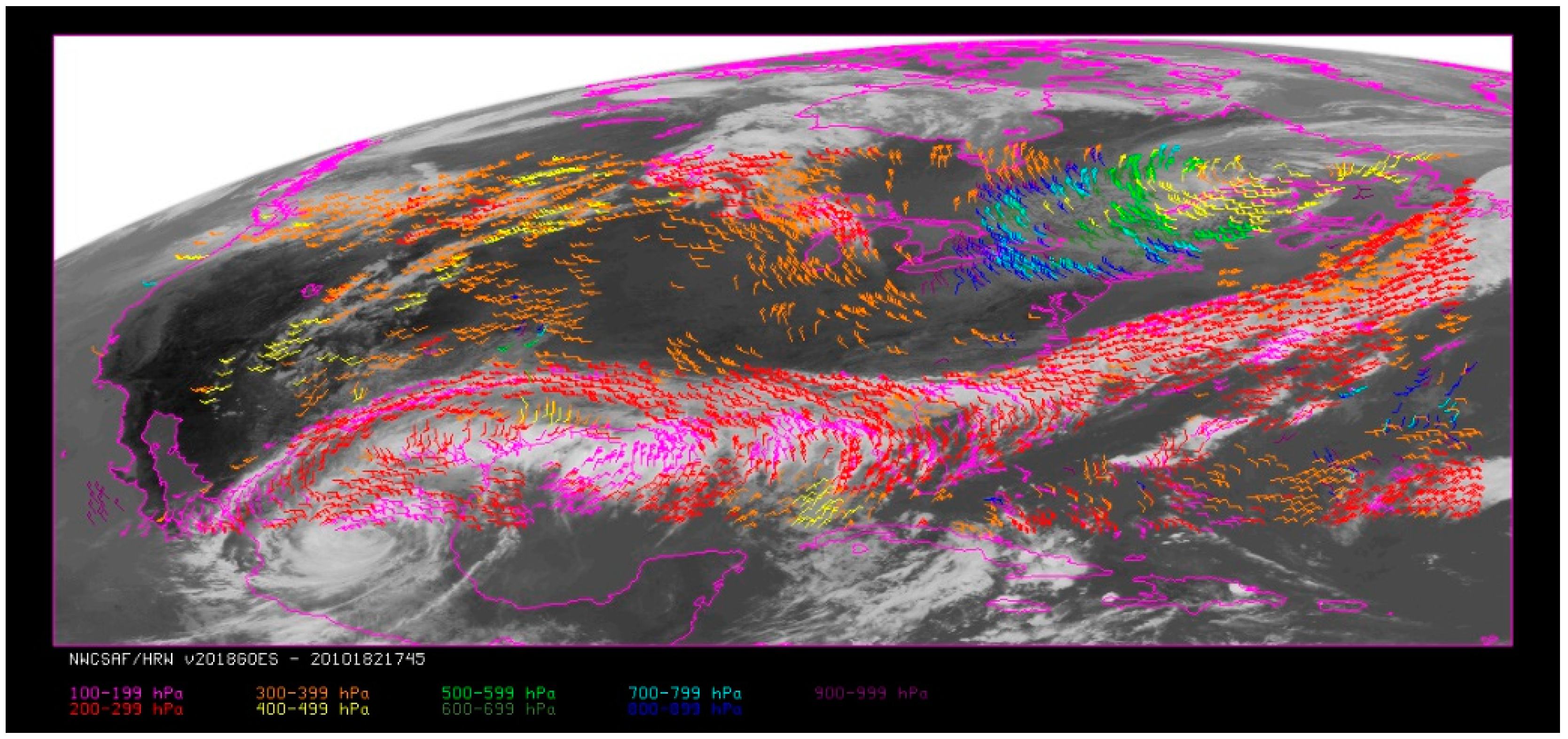
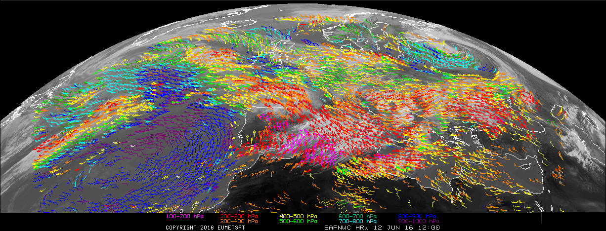
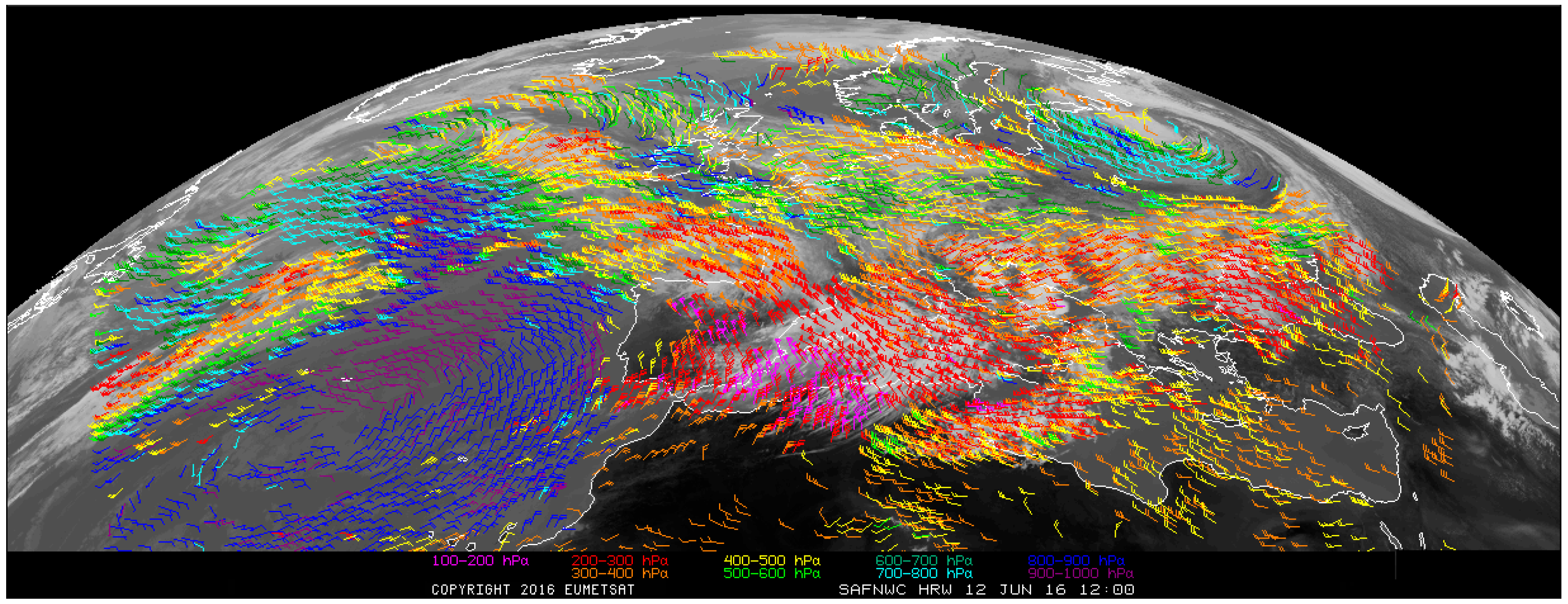
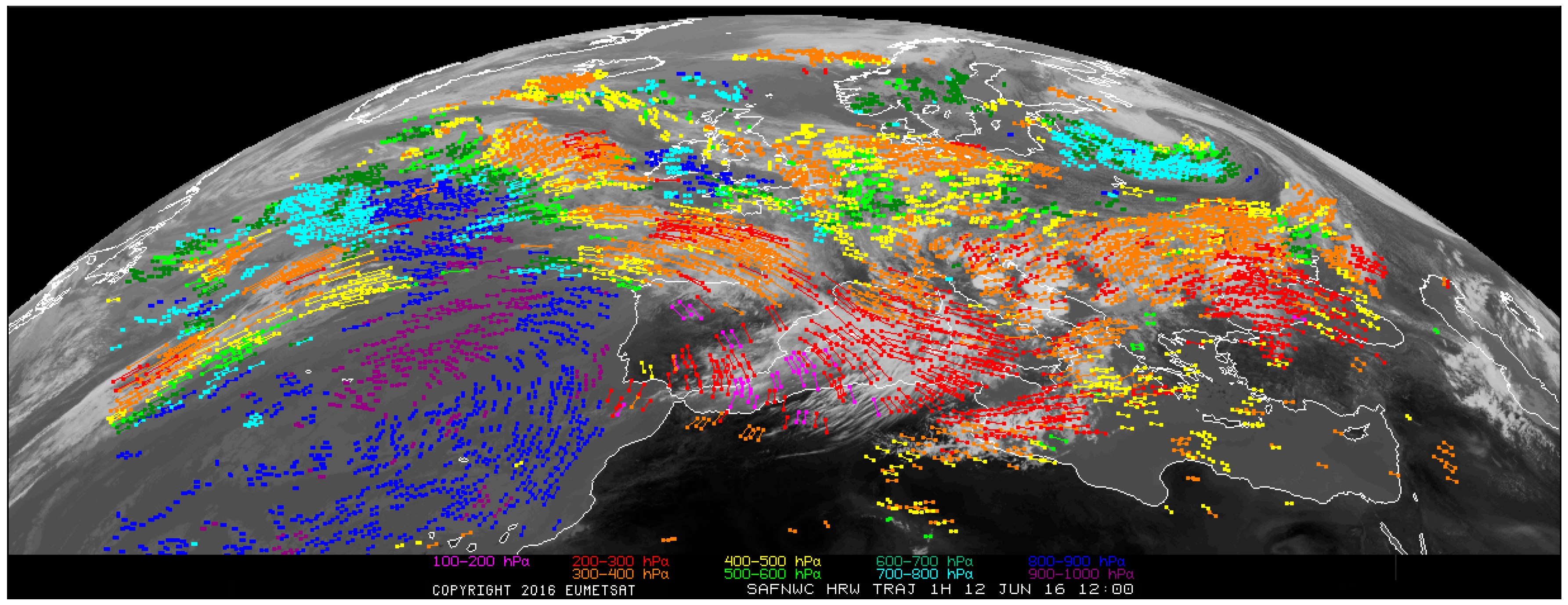
4.4. Real Time Output of NWC/GEO-HRW Product

Real time graphic displays of NWC/GEO-HRW latest version AMVs and trajectories, generated by the NWC/GEO reference system with MSG satellite series 24 h a day, are available at the NWCSAF Help Desk website (http://www.nwcsaf.org). The specific links for HRW outputs are:

5. Conclusions

Considering NWCSAF High Resolution Winds (NWC/GEO-HRW) product for calculation of AMVs and trajectories, inside its NWC/GEO software package for geostationary satellites:
  • It is easy to get, install and use. It is fully portable and independent from external applications.
  • The code is fairly easy to read (with functions written in C and Fortran languages, and a code extensively commented to help its understanding), and fully documented.
  • There is a fully dedicated Helpdesk where NWCSAF users find support and help on the installation and use of the software.
  • It has been adapted to MSG, Himawari-8/9, GOES-N, and GOES-R satellite series.
  • Comparing the validation for all satellite series, equivalent validation statistics are obtained for all of them, and so NWC/GEO-HRW product can be used with the same quality throughout all the planet Earth with all the considered satellites.
  • In the ‘2014 and 2018 AMV Intercomparison Studies’ [19,23], NWC/GEO-HRW is one of the two best AMV algorithms for both MSG and Himawari-8/9 satellites, calculating a high number of AMVs with very good validation statistics.
With this, NWCSAF High Resolution Winds (NWC/GEO-HRW) becomes a very useful source of AMVs and trajectories for the weather analysis and forecasting. It is useful for the monitoring of the general atmospheric flow, of small-scale circulation and wind singularities, of convergence at low levels or divergence at the top of developed systems. It is also useful for the watch and warning of dangerous wind situations. It can also be used in form of objectively derived fields, assimilated in numerical weather prediction models together with many other data, or used as an input in analysis and forecast applications.
The ‘Coordination Group for Meteorological Satellites (CGMS)’ has officially also recognized in its ‘2012 Meeting Report’ [27] (p. 117):
  • NWCSAF High Resolution Winds fulfills the requirements to be a portable stand-alone AMV calculation software due to its easy installation and usability.
  • It has been successfully adapted by some CGMS members and serves as an important tool for development. It is modular, well documented, and well suited as stand-alone AMV software.
  • Although alternatives exist as portable stand-alone AMV calculation software, they are not as advanced in terms of documentation and do not have an existing Helpdesk.
With this, NWCSAF High Resolution Winds (NWC/GEO-HRW) is a ready-to-go starting point for the derivation of winds from satellite measurements for the research community. It can serve as focal point for sharing and comparing code among different research groups. This could lead to a better understanding of AMVs, future AMV algorithm enhancements, and improvements in the performance of operationally derived AMVs.
Operational meteorologists and researchers are recommended to register as NWCSAF users, and to use NWC/GEO software package and NWC/GEO-HRW High Resolution Winds product. It is especially recommended for those without access to AMV products similar to it, and who might benefit from its use. Feedback is also very welcome.

Author Contributions

Conceptualization, methodology, and software: J.G.-P. (major contributions to NWC/GEO-HRW product since 2005), J.M.F.-S. (major contributions to NWC/GEO-HRW product between 1997 and 2005), Ó.A. (major contributions to NWC/GEO software package and minor contributions to NWC/GEO-HRW product throughout all the development period), A.S., R.G., C.A., I.S., L.F. (major contributions to NWC/GEO software package and minor contributions to NWC/GEO-HRW product throughout smaller periods); Formal analysis: J.G.-P. and J.M.F.-S.; Validation: J.G.-P.; Writing—original draft preparation and review and editing: J.G.-P.

Funding

This research is funded by the “European Organisation for the Exploitation of Meteorological Satellites (EUMETSAT)” and “Agencia Estatal de Meteorología (AEMET)”, through the “Satellite Application Facility on Support to Nowcasting and very short range forecasting (NWCSAF)” program. The Article Processing Charge (APC) is funded by “Agencia Estatal de Meteorología (AEMET)”. The researchers want to recognize the clear technical and financial support by EUMETSAT and AEMET for the development of NWC/GEO software package and NWC/GEO-HRW High Resolution Winds product for more than 20 years, the continuity of this support in the coming years for additional improvements in NWC/GEO-HRW product, and its extension to other satellite series like MTG-Imager.

Acknowledgments

The researchers want to acknowledge the support shown by the International Winds Working Group (IWWG) for the improvement and promotion of NWC/GEO-HRW product. This acknowledgment is especially dedicated to the IWWG co-chairs since 2006: Régis Borde (EUMETSAT), Steve Wanzong (SSEC/UW), Mary Forsythe (Met Office), Jaime Daniels (NOAA), Kenneth Holmlund (EUMETSAT), and Chris Velden (SSEC/UW).

Conflicts of Interest

The authors declare no conflict of interest.

Abbreviations

AEMETAgencia Estatal de Meteorología of Spain (National Weather Service)
AMVAtmospheric Motion Vector
ANMAdministraţia Naţională de Meteorologie of Romania
CALIPSONASA & CNES Cloud-Aerosol Lidar and Infrared Pathfinder Satellite Observations
CGMSCoordination Group for Meteorological Satellites
CMAChina Meteorological Administration
CNESFrance Centre National d’Études Spatiales
CPTEC/INPEBrazil National Institute for Space Research Center for Weather Forecasting and Climate Studies
ECMWFEuropean Center for Medium-Range Weather Forecasts
EUMETSATEuropean Organization for Exploitation of Meteorological Satellites
GOES-NNOAA Second Generation of Geostationary Operational Environmental Satellites (GOES-13, GOES-14, GOES-15)
GOES-RNOAA Third Generation of Geostationary Operational Environmental Satellites (GOES-16, GOES-17, GOES-T, GOES-U)
Himawari-8/9JMA Himawari third generation of geostationary satellites
IWWGInternational Winds Working Group
JMAJapan Meteorological Agency
KMAKorea Meteorological Administration
MFMétéo-France
MSGEUMETSAT Meteosat Second Generation of geostationary satellites
NASAUnited States National Aeronautics and Space Administration
NBIASNormalized bias (explained in Appendix A).
NCNumber of collocations (explained in Appendix A).
NMVDNormalized mean vector difference (explained in Appendix A).
NOAAUnited States National Oceanic and Atmospheric Administration
NOAA/NCEPNOAA National Centers for Environmental Prediction
NRMSVDNormalized root mean square vector difference (explained in Appendix A).
NWC/GEONWCSAF software package for geostationary satellites
NWC/GEO-CloudNWC/GEO Cloud products: Cloud Mask (CMA), Cloud Type (CT), Cloud Top Temperature and Height (CTTH), Cloud Microphysics (CMIC)
NWC/GEO-HRWNWC/GEO High Resolution Winds product
NWC/PPSNWCSAF software package for polar satellites
NWCSAFEUMETSAT Satellite Application Facility on support to nowcasting and very short range forecasting
NWPNumerical Weather Prediction
OSTIAOperational Sea Surface Temperature and Sea Ice Analysis
SMHISveriges Meteorologiska och Hydrologiska Institut of Sweden
SPDMean horizontal speed for reference winds (explained in Appendix A).
SSEC/UWUniversity of Wisconsin-Madison Space Science and Engineering Center
WMOWorld Meteorological Organization
ZAMGZentralanstalt für Meteorologie und Geodynamik of Austria

Appendix A

NWC/GEO-HRW Validation Statistics
The validation statistics defined at the Third and Fourth International Winds Workshops [21,22], and recommended by the Coordination Group for Meteorological Satellites (CGMS) for the international comparison of satellite winds, are used in this paper:
  • NC (dimensionless): Number of collocations between the NWC/GEO-HRW AMV winds, defined as (Ui,Vi), and the radiosonde reference winds, defined as (Ur,Vr). Speed components for both types of winds defined in m/s units.
  • SPD (in m/s units): Mean horizontal speed for the reference radiosonde winds.
  • BIAS (in m/s units): Difference between the mean horizontal wind speed of the reference winds and the collocated NWC/GEO-HRW AMV winds
    BIAS = (Σ((Ui2 + Vi2)1/2 − (Ur2 + Vr2)1/2))/NC
It estimates the systematic error related to the calculation of the AMV wind speed (over- or underestimation of the mean AMV wind speed with respect to the mean reference wind speed).
• MVD (in m/s units): Mean vector difference between the reference winds and the AMV winds
MVD = (ΣVDi)/NC
where
VDi = ((Ui − Ur)2 + (Vi − Vr)2)1/2
It estimates the systematic error related to the calculation of the AMV wind vectors.
• RMSVD (in m/s units): Root mean square vector difference
RMSVD = (MVD2 + SD2)1/2
where
SD = ((Σ(VDi − MVD)2)/NC)1/2
It estimates the systematic and random error related to the calculation of the AMV wind vectors. It is calculated through the mean vector difference (MVD), and the standard deviation (SD) of each vector difference with respect to the mean.
AMVs are compared to the nearest radiosonde wind with a maximum distance of 150 km and a maximum pressure difference of 25 hPa. Due to the variable magnitude the parameters can have in different samples, SPD parameter is used for normalization. This way, the following relative parameters based on the previous ones are used in the validation; these parameters are independent of the magnitude of the winds and can more easily be compared in different samples of data:
  • NBIAS (dimensionless) = BIAS/SPD (normalized bias).
  • NMVD (dimensionless) = MVD/SPD (normalized mean vector difference).
  • NRMSVD (dimensionless) = RMSVD/SPD (normalized root mean square vector difference).

References

  1. EUMETSAT Operational Services Specification, v2H, June 2018 (Document Code EUM/OPS/SPE/09/0810). Available online: https://www.eumetsat.int/website/home/Data/TechnicalDocuments/index.html (accessed on 24 August 2019).
  2. Definitions of Meteorological Forecasting Ranges. Manual on the Global Data-Processing and Forecasting System, Appendix I.4. World Meteorological Organization Publication WMO-No. 485. 1992. Available online: https://www.wmo.int/pages/prog/www/DPS/Publications/WMO_485_Vol_I.pdf (accessed on 24 August 2019).
  3. García-Pereda, J.; Borde, R. NWCSAF High Resolution Winds as stand-alone AMV calculation software. In Proceedings of the 11th International Winds Workshop, Auckland, New Zealand, 20–24 February 2012. [Google Scholar]
  4. Stark, J.D.; Donolon, C.J.; Martin, M.J.; McCulloch, M.E. OSTIA: An operational, high resolution, real time, global sea surface temperature analysis system. In Proceedings of the Oceans’07 IEEE Conference, Aberdeen, UK, 18–21 June 2007. [Google Scholar]
  5. OSTIA Data Home Page. Available online: http://ghrsst-pp.metoffice.com/pages/latest_analysis/ostia.html (accessed on 24 August 2019).
  6. Hayden, C.M.; Merrill, R.T. Recent NESDIS research in wind estimation from geostationary satellite images. In Proceedings of the ECMWF Seminar: Data assimilation and the Use of Satellite Data, Reading, UK, 5–9 September 1988. [Google Scholar]
  7. Borde, R.; Carranza, M.; García-Pereda, J.; Nonaka, K.; Oh, S.M.; Bailey, A.; Wanzong, S.; Galante-Negri, R. International Winds Working Group Operational AMV Production Survey (December 2018). Available online: http://cimss.ssec.wisc.edu/iwwg/Docs/AMVSURVEY2018_TOTAL.pdf (accessed on 24 August 2019).
  8. Xu, J.; Zhang, Q. Calculation of Cloud motion wind with GMS-5 images in China. In Proceedings of the 3rd International Winds Workshop, Ascona, Switzerland, 10–12 June 1996. [Google Scholar]
  9. Borde, R.; Oyama, R. A direct link between feature tracking and height assignment of operational AMVs. In Proceedings of the 9th International Winds Workshop, Annapolis, MD, USA, 14–18 April 2008. [Google Scholar]
  10. Le Gléau, H. Algorithm Theoretical Basis Document for the Cloud Product Processors of the NWC/GEO (January 2019). Available online: http://www.nwcsaf.org/aemetRest/downloadAttachment/5362 (accessed on 24 August 2019).
  11. Sèze, G.; Pelon, J.; Derrien, M.; Le Gléau, H.; Six, B. Evaluation against CALIPSO lidar observations of the multi-geostationary cloud cover and type data set assembled in the framework of the MEGHA-TROPIQUES mission. Q. J. R. Meteorol. Soc. 2015, 141, 774–797. [Google Scholar] [CrossRef]
  12. Hamann, U.; Walther, A.; Baum, B.; Bennartz, R.; Bugliaro, L.; Derrien, M.; Francis, P.N.; Heidinger, A.; Joro, S.; Kniffka, A.; et al. Remote sensing of cloud top pressure/height from SEVIRI: Analysis of ten current retrieval algorithms. Atmos. Meas. Tech. 2014, 7, 2839–2867. [Google Scholar] [CrossRef]
  13. Choi, Y.S; Heidinger, A.; Walther, A. Assessment of cloud parameter retrievals from Himawari-8 geostationary imagery. In Proceedings of the 2nd International Cloud Working Group Workshop, Madison, WI, USA, 29 October–2 November 2018. [Google Scholar]
  14. Lean, P.; Kelly, G.; Migliorini, S. Characterizing AMV height assignment errors in a simulation study. In Proceedings of the 12th International Winds Workshop, Copenhagen, Denmark, 16–20 June 2014. [Google Scholar]
  15. Hernández-Carrascal, Á.; Bormann, N. Cloud top, Cloud center, Cloud layer—Where to place AMVs? In Proceedings of the 12th International Winds Workshop, Copenhagen, Denmark, 16–20 June 2014. [Google Scholar]
  16. Salonen, K.; Bormann, N. Investigations of alternative interpretations of AMVs. In Proceedings of the 12th International Winds Workshop, Copenhagen, Denmark, 16–20 June 2014. [Google Scholar]
  17. García-Pereda, J. Algorithm Theoretical Basis Document for the Wind Product Processor of the NWC/GEO (January 2019). Available online: http://www.nwcsaf.org/aemetRest/downloadAttachment/5449 (accessed on 24 August 2019).
  18. Holmlund, K. The utilisation of statistical properties of satellite derived Atmospheric Motion Vectors to derive Quality Indicators. Weather Forecast. 1998, 13, 1093–1104. [Google Scholar] [CrossRef]
  19. Santek, D.; Dworak, R.; Wanzong, S.; Johnson, K.; Nebuda, S.; García-Pereda, J.; Borde, R.; Carranza, M. Third AMV Intercomparison Study. In Proceedings of the 14th International Winds Workshop, Jeju, Korea, 23–27 April 2018. [Google Scholar]
  20. Salonen, K.; Cotton, J.; Bormann, N.; Forsythe, M. Characterising AMV height assignment error by comparing best fit pressure statistics from the Met Office and ECMWF system. In Proceedings of the 11th International Winds Workshop, Auckland, New Zealand, 20–24 February 2012. [Google Scholar]
  21. Menzel, W.P. Report from the Working Group on Verification Statistics. In Proceedings of the 3rd International Winds Workshop, Ascona, Switzerland, 10–12 June 1996. [Google Scholar]
  22. Velden, C.; Holmlund, K. Report from the Working Group on Verification and Quality Indices. In Proceedings of the 4th International Winds Workshop, Saanenmoser, Switzerland, 20–23 October 1998. [Google Scholar]
  23. Santek, D.; García-Pereda, J.; Velden, C.; Genkova, I.; Stettner, D.; Wanzong, S.; Nebuda, S.; Mindock, M. A new Atmospheric Motion Vector Intercomparison Study. In Proceedings of the 12th International Winds Workshop, Copenhagen, Denmark, 16–20 June 2014. [Google Scholar]
  24. Alonso, Ó.; Fernández, L. User Manual for the NWC/GEO: Software Part (January 2019). Available online: http://www.nwcsaf.org/aemetRest/downloadAttachment/5413 (accessed on 24 August 2019).
  25. García-Pereda, J. User Manual for the Wind Product Processor of the NWC/GEO: Science Part (January 2019). Available online: http://www.nwcsaf.org/aemetRest/downloadAttachment/5451 (accessed on 24 August 2019).
  26. García-Pereda, J. Scientific and Validation Report for the Wind Product Processor of the NWC/GEO (January 2019). Available online: http://www.nwcsaf.org/aemetRest/downloadAttachment/5453 (accessed on 24 August 2019).
  27. Coordination Group on Meteorological Satellites (CGMS). Report of 40th Meeting. Lugano, Switzerland, November 2012. Available online: https://www.cgms-info.org/documents/cgms-40-report.pdf (accessed on 24 August 2019).
Figure 1. NWC/GEO-HRW output example of atmospheric motion vectors (AMVs) in the European and North Atlantic region, considering the default conditions for processing (12 June 2016, 12:00 UTC, MSG-3 satellite). Color coding based on the AMV pressure.
Remotesensing 11 02032 g001
Figure 2. NWC/GEO-HRW output example of 1-h trajectories in the European and North Atlantic region, considering the default conditions for processing (12 June 2016, 12:00 UTC, MSG-3 satellite). Color coding based on the AMV pressure.
Remotesensing 11 02032 g002
Figure 3. ‘Basic scale AMVs’ (in red and green, related to the tracer calculation method used for their extraction), in a single scale NWC/GEO-HRW example for the European and Mediterranean region, with the default conditions for MSG satellites (14 May 2010, 12:00 UTC, MSG-2 satellite).
Remotesensing 11 02032 g003
Figure 4. ‘Basic scale AMVs’ (in red), and ‘detailed scale AMVs’ (in yellow, green, and blue, considering their relationship with the basic scale AMVs), in a two-scale NWC/GEO-HRW example for the European and Mediterranean region, with the default conditions for MSG satellites (14 May 2010, 12:00 UTC, MSG-2 satellite).
Remotesensing 11 02032 g004
Figure 5. AMVs related to the satellite channel used for the AMV calculation, in a NWC/GEO-HRW example for the European and Mediterranean region, with the default conditions for MSG satellites (14 May 2010, 12:00 UTC, MSG-2 satellite).
Remotesensing 11 02032 g005
Figure 6. A low resolution tracer for 16 December 2009 11:45 UTC (red square, with its center in the red mark), the location of its center defined by NWP wind guess at 12:00 UTC (yellow mark), and its true tracking center at 12:00 UTC defined by NWC/GEO-HRW product (blue mark), for an example case of AMVs with MSG-2 satellite. The yellow square (with its center at the position defined by the NWP wind guess at 12:00 UTC) corresponds to the tracking area using the wind guess for its definition. The green square (with its center at the position of the tracer at 11:45 UTC) corresponds to the tracking area not using the wind guess for its definition. The larger size of the tracking area when the wind guess has not been used is to be noticed, which causes a longer time for the running of NWC/GEO-HRW product, but at the same time reduces the dependence from the NWP model.
Remotesensing 11 02032 g006
Figure 7. Matrices and graphs used in the calculation of CCC method height assignment, for a MSG/VIS08 case (a) and a MSG/IR108 case (b), as explained in the text. Pixels and graphs actually used for the calculations of PCCC and ΔPCCC are those included in the blue squares. The weighted location used for the calculation of the AMV displacement between the initial image and the later image is also shown as a red cross in the images in the first row.
Remotesensing 11 02032 g007
Figure 8. Graphs relating for MSG satellites the difference between the AMV pressure level calculated with CCC method and the AMV best fit pressure level (in 103 hPa) in red, the NBIAS in yellow and the NRMSVD in blue (both dimensionless), with the AMV ice/liquid water path (in kg/m2), for ice visible AMVs (a), ice infrared AMVs (b), ice water vapor AMVs (c), liquid visible AMVs (d), liquid infrared AMVs (e), and liquid water vapor AMVs (f). 12:00 UTC Cloudy AMVs for MSG-2 satellite for July 2010–June 2011 in the European and Mediterranean region used for the tuning. NBIAS and NRMSVD parameters used as defined in Appendix A.
Remotesensing 11 02032 g008
Figure 9. AMV height assignment (CCC method with or without microphysics correction, using the high or low CCC method calculation threshold), and AMV phase (ice cloud AMV, liquid cloud AMV, mixed/undefined cloud AMV, clear air AMV), in a NWC/GEO-HRW example for the European and Mediterranean region, with the default conditions for MSG satellites (14 May 2010, 12:00 UTC, MSG·2 satellite).
Remotesensing 11 02032 g009
Figure 10. AMV pressure correction (for the cases in which CCC method with microphysics correction height assignment has been used), in a NWC/GEO-HRW example for the European and Mediterranean region, with the default conditions for MSG satellites (14 May 2010, 12:00 UTC, MSG·2 satellite).
Remotesensing 11 02032 g010
Figure 11. Quality indicator with forecast values, for the NWC/GEO-HRW example for the European and Mediterranean region, with the default conditions for MSG satellites (14 May 2010, 12:00 UTC, MSG-2 satellite). Only values for quality indicator without forecast ≥ 70% are present, because of the use of this threshold for the AMV filtering.
Remotesensing 11 02032 g011
Figure 12. Common quality indicator without forecast values, for the NWC/GEO-HRW example for the European and Mediterranean region, with the default conditions for MSG satellites (14 May 2010, 12:00 UTC, MSG-2 satellite). The differences with Figure 11, and the fact that not all AMVs have a valid value for the common quality indicator without forecast are to be noticed.
Remotesensing 11 02032 g012
Figure 13. NWC/GEO-HRW v2018.1 AMV output example in the European and Mediterranean region considering the default conditions for processing (14 May 2010, 12:00 UTC, MSG-2 satellite). Color coding based on the AMV pressure.
Remotesensing 11 02032 g013
Figure 14. NWC/GEO-HRW v2018.1 AMV output example in the China/Korea/Japan region considering the default conditions for processing (2 April 2018, 00:00 UTC, Himawari-8 satellite). Color coding based on the AMV pressure.
Remotesensing 11 02032 g014
Figure 15. NWC/GEO-HRW v2018.1 AMV output example in the Continental United States region considering the default conditions for processing (1 July 2010, 17:45 UTC, GOES-13 satellite). Color coding based on the AMV pressure.
Remotesensing 11 02032 g015
Figure 16. NWC/GEO-HRW v2018.1 AMV output example in the continental United States region considering the default conditions for processing (22 May 2018, 00:00 UTC, GOES-16 satellite, mode 3 scanning). Color coding based on the AMV pressure.
Remotesensing 11 02032 g016
Table 1. AMV filtering related to the AMV cloud types (in rows) and the satellite channels used for the AMV calculation (in columns), and consideration of the cloud top pressure (T) or cloud representative pressure (R) in the EBBT height assignment method for the AMV pressure.
MSG ChannelHR VISVIS 06VIS 08IR 108IR 120WV 62WV 73
GOES-N ChannelVIS 07IR 107WV 65
Himawari-8/9 or GOES-R ChannelVIS 06VIS 08IR 112WV 62WV 70WV 74
Cloud free land/sea TTT
Land/sea contaminated by ice TTT
Very low/low cumulus/stratusRRRRRR RR
Medium cumulus/stratusRRRRRR RR
High/Very high cumulus/statusRR RRRRR
Fractional clouds
High semitransparent thin TTTTT
High semitransparent meanly thickTT TTTTT
High semitransparent thickRR RRRRR
High semitransparent over cloud/ice TTRRR
Multiple cloud typesRR RRRRR
Multiple clear air types TTT
Mixed cloudy/clear air typesRR RRRRR
Unprocessed cloud typeRRRRRRRRR
Table 2. Correction for the AMV pressure (in hPa), based on the AMV Ice water path (IWPccc) or AMV Liquid water path (LWPccc) values (in kg/m2), for MSG satellite series.
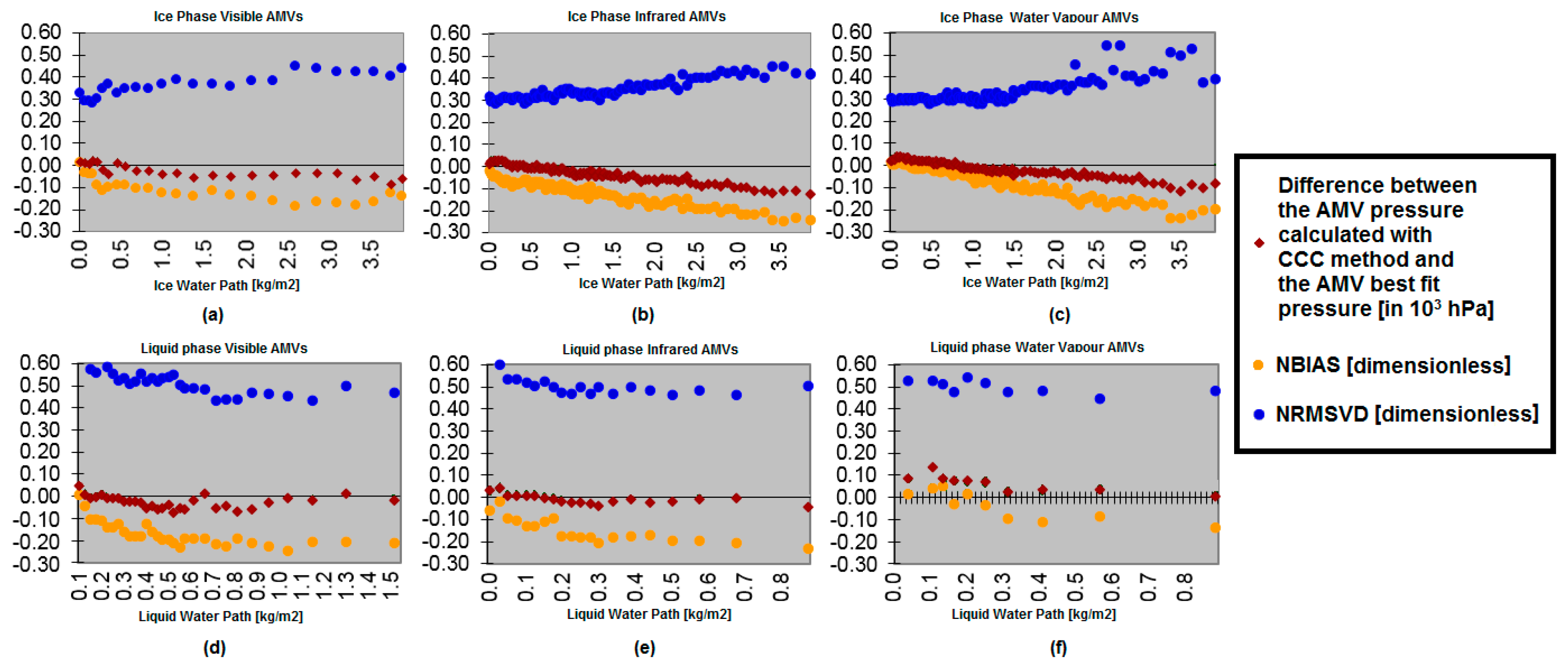
Correction for the AMV Pressure (in hPa) for MSG Satellite Series, Based on the AMV Ice Water Path (IWPccc) or AMV Liquid Water Path (LWPccc)
VISIBLE ICE PHASE CLOUDY AMVSVISIBLE LIQUID PHASE CLOUDY AMVS
Corr.[hPa] = 51 without IWPcccCorr.[hPa] = 16 without LWPccc
Corr.[hPa] = −14 + 48·IWPccc[kg/m2]Corr.[hPa] = −42 + 226·LWPccc [kg/m2]
if IWPccc < 1.3542 kg/m2if LWPccc < 0.3540 kg/m2
Corr.[hPa] = 51 if IWPccc ≥ 1.3542 kg/m2Corr.[hPa] = 38 if LWPccc ≥ 0.3540 kg/m2
INFRARED ICE PHASE CLOUDY AMVSINFRARED LIQUID PHASE CLOUDY AMVS
Corr.[hPa] = 10 without IWPcccCorr.[hPa] = 9 without LWPccc
Corr.[hPa] = −16 + 37·IWPccc[kg/m2]Corr.[hPa] = −36 + 251·LWPcccc[kg/m2]
if IWPccc < 3.3514 kg/m2if LWPccc < 0.2271 kg/m2
Corr.[hPa] = 108 if IWPccc ≥ 3.3514 kg/m2Corr.[hPa] = 21 if LWPccc ≥ 0.2271 kg/m2
WATER VAPOR ICE PHASE CLOUDY AMVSWATER VAPOR LIQUID PHASE CLOUDY AMVS
Corr.[hPa] = −7 without IWPcccCorr.[hPa] = −56 without LWPccc
Corr.[hPa] = −29 + 34·IWPccc[kg/m2]Corr.[hPa] = −109 + 202·LWPccc[kg/m2]
if IWPccc < 3.3824 kg/m2if LWPccc < 0.5149 kg/m2
Corr.[hPa] = 86 if IWPccc ≥ 3.3824 kg/m2Corr.[hPa] = −5 if LWPccc ≥ 0.5149 kg/m2
Table 3. AMV filtering related to the AMV pressure (in rows) and the satellite channels used for the AMV calculation (in columns). ‘C’ means clear air AMVs removed; ‘A’ means all AMVs removed; ‘L’ means all AMVs removed if so configured (not in the default configuration).
MSG ChannelHRVISVIS06VIS08IR 108IR 120WV62WV73
GOES-N ChannelVIS07IR 107WV65
Himawari-8/9 or GOES-R ChannelVIS06VIS08IR 112WV62WV70WV74
100–199 hPa AA
200–299 hPa AA
300–399 hPa AA
400–499 hPa CCC
500–599 hPa ACC
600–699 hPa ACC
700–799 hPa AAA
800–899 hPa AAA
900–999 hPa LLAAA
Table 4. Validation for NWC/GEO-HRW v2018.1 AMVs against radiosonde winds, considering all AMVs together and in three separate layers: high levels: 100–400 hPa; medium levels: 400–700 hPa; low levels: 700–1000 hPa (Jul 2009–Jun 2010, 12:00 UTC, MSG-2 satellite, European and Mediterranean region).
HRWv2018.1
MSG-2
Jul‘09–Jun‘10
Cloudy
HRVIS
Cloudy
VIS06
Cloudy
VIS08
Cloudy
IR108
Cloudy
IR120
Cloudy
WV62
Cloudy
WV73
Clear AirAll AMVs
ALL LEVELS
NC67,28898,86190,082226,314228,664139,042227,27320,3831,097,907
SPD (m/s)12.8710.2810.2517.5017.7222.7820.1417.4217.23
NBIAS−0.03−0.13−0.13−0.08−0.07−0.02−0.05+0.01−0.07
NMVD0.350.410.420.300.300.260.290.300.32
NRMSVD0.420.490.490.370.370.320.360.370.39
HIGH LEVELS
NC15,919 119,091124,905128,731157,68920,383566,718
SPD (m/s)21.13 21.8521.8123.2322.6317.4222.19
NBIAS−0.03 −0.07−0.06−0.03−0.06+0.01−0.05
NMVD0.25 0.260.260.260.260.300.26
NRMSVD0.30 0.320.320.320.320.370.32
MED. LEVELS
NC15,44731,34629,70065,54464,17910,31160,432 276,959
SPD (m/s)12.8811.7211.4914.2914.4417.1314.95 13.91
NBIAS−0.05−0.15−0.16−0.09−0.08+0.04−0.02 −0.08
NMVD0.350.380.380.350.350.360.37 0.36
NRMSVD0.420.450.460.430.430.440.46 0.44
LOW LEVELS
NC35,92267,51560,38241,67939,580 9152 254,230
SPD (m/s)9.219.619.6310.1110.14 11.51 9.79
NBIAS−0.02−0.11−0.11−0.11−0.10 −0.02 −0.09
NMVD0.450.430.440.400.40 0.41 0.42
NRMSVD0.530.510.510.480.47 0.48 0.50
Table 5. Validation for NWC/GEO-HRW v2018.1 AMVs against radiosonde winds, considering all AMVs together and in three separate layers: high levels: 100–400 hPa; medium levels: 400–700 hPa; low levels: 700–1000 hPa (Mar 2018–Aug 2018, 00:00 UTC, Himawari-8 satellite, China/Korea/Japan region).
HRW v2018.1
Himawari-8
Mar–Aug’18
Cloudy
VIS06
Cloudy
VIS08
Cloudy
IR112
Cloudy
WV62
Cloudy
WV70
Cloudy
WV74
Clear AirAll AMVs
ALL LEVELS
NC36,84171,618287,147189,457246,356280,89985,1481,197,466
SPD (m/s)21.7019.9519.5823.6022.5821.9419.3221.46
NBIAS0.000.00+0.04+0.06+0.06+0.04+0.06+0.05
NMVD0.240.260.270.260.270.260.300.28
NRMSVD0.290.310.350.320.330.330.380.35
HIGH LEVELS
NC26,76948,276196,718183,124214,714229,29185,148984,040
SPD (m/s)25.8324.5222.6123.7323.4423.3119.3223.06
NBIAS−0.01−0.01+0.04+0.06+0.05+0.03+0.06+0.04
NMVD0.220.230.250.260.260.250.300.25
NRMSVD0.260.270.310.310.310.300.380.31
MED. LEVELS
NC4200950765,466633331,64251,608 168,756
SPD (m/s) 14.6714.1814.6820.0816.7215.85 15.60
NBIAS+0.10+0.09+0.05+0.17+0.21+0.11 +0.11
NMVD0.320.330.350.360.430.38 0.37
NRMSVD0.400.420.490.470.540.50 0.50
LOW LEVELS
NC587213,83524,963 44,670
SPD (m/s) 7.907.978.53 8.27
NBIAS−0.03+0.03−0.01 0.00
NMVD0.440.470.43 0.45
NRMSVD0.540.580.53 0.55
Table 6. Validation for NWC/GEO-HRW v2018.1 AMVs against radiosonde winds, considering all AMVs together and in three separate layers: high levels: 100–400 hPa; medium levels: 400–700 hPa; low levels: 700–1000 hPa (Jul 2010–Jun 2011, 05:45/11:45/17:45/23:45 UTC, GOES-13 satellite, continental United States region).
HRW v2018.1
GOES-13
Jul’10–Jun’11
Cloudy
VIS07
Cloudy
IR107
Cloudy
WV65
Clear AirAll AMVs
ALL LEVELS
NC9282287,572247,35064,486608,690
SPD (m/s)21.3321.8225.2214.6422.43
NBIAS−0.01−0.08−0.04+0.04−0.05
NMVD0.240.290.260.370.28
NRMSVD0.310.370.330.490.36
HIGH LEVELS
NC6828215,848235,43964,486522,601
SPD (m/s)25.2824.7425.4414.6423.82
NBIAS−0.01−0.09−0.04+0.04−0.05
NMVD0.230.280.260.370.28
NRMSVD0.280.350.330.490.35
MED. LEVELS
NC24333,93311,911 46,087
SPD (m/s)18.2917.0420.84 18.03
NBIAS−0.11−0.050.00 −0.03
NMVD0.340.350.29 0.33
NRMSVD0.450.430.37 0.41
LOW LEVELS
NC221137,791 40,002
SPD (m/s)9.469.44 9.44
NBIAS−0.02−0.09 −0.09
NMVD0.350.40 0.39
NRMSVD0.430.49 0.49
Table 7. Validation for NWC/GEO-HRW v2018.1 AMVs against radiosonde winds, considering all AMVs together and in three separate layers: high levels: 100–400 hPa; medium levels: 400–700 hPa; low levels: 700–1000 hPa (Mar 2018–Aug 2018, 00:00/12:00 UTC, GOES-16 satellite, continental United States region).
HRW v2018.1
GOES-16
Mar–Aug’18
Cloudy
VIS06
Cloudy
VIS08
Cloudy
IR112
Cloudy
WV62
Cloudy
WV70
Cloudy
WV74
Clear AirAll AMVs
ALL LEVELS
NC863031,657416,089330,893401,488433,933171,8701,794,560
SPD (m/s)22.3620.3020.0723.4322.7922.3816.8421.57
NBIAS+0.010.00+0.04+0.05+0.04+0.02+0.06+0.04
NMVD0.230.250.270.260.260.260.320.27
NRMSVD0.280.310.340.320.320.320.410.34
HIGH LEVELS
NC695223,845300,271316,898353,596367,433171,8701,540,865
SPD (m/s)25.0623.0222.1223.6023.4323.2616.8422.44
NBIAS0.000.00+0.04+0.04+0.03+0.02+0.06+0.03
NMVD0.210.230.260.250.250.240.320.26
NRMSVD0.260.280.320.310.310.300.410.32
MED. LEVELS
NC638336877,91513,99547,89266,500 210,308
SPD (m/s)17.3315.8116.8619.5918.0717.51 17.51
NBIAS+0.09+0.06+0.03+0.15+0.16+0.09 +0.09
NMVD0.290.300.310.360.380.35 0.34
NRMSVD0.380.370.400.450.480.43 0.43
LOW LEVELS
NC1040444437,903 43,387
SPD [m/s]7.419.0910.46 10.25
NBIAS+0.170.00−0.02 −0.02
NMVD0.630.440.38 0.39
NRMSVD0.760.540.47 0.48
Table 8. Environments used for development and testing of NWC/GEO v2018.1 software package.
Environment Used for Development and TestingEnvironment Used for Testing
Operative SystemLinux RHEL release 6.4 (Santiago)Ubuntu 18.04.1 LTS
CPU4 × Intel® Core™8 × Intel® Xeon®
CPU i5–4590 @ 3.30 GhzCPU E5–2650 v3 @ 2.30 Ghz
Architecturex86_64x86_64
Memory16 GB16 GB
Disk500 GB500 GB
Shellsbash; kshsh; ksh
CompilersGCC compilers 4.4.7:GCC compilers 7.3.0:
gcc; g++; gfortrangcc; g++; gfortran
gzipgzip 1.3.12gzip 1.6
makeGNU Make 3.81GNU Make 4.1

