Earth Observations-Based Evapotranspiration in Northeastern Thailand


State Key Laboratory of Remote Sensing Science, Institute of Remote Sensing and Digital Earth, Chinese Academy of Sciences, Beijing 100101, China
*
Author to whom correspondence should be addressed.
Remote Sens. 2019, 11(2), 138; https://doi.org/10.3390/rs11020138
Submission received: 5 December 2018
/
Revised: 2 January 2019
/
Accepted: 8 January 2019
/
Published: 12 January 2019
(This article belongs to the Special Issue Remote Sensing of Evapotranspiration (ET))
Abstract
:Thailand is characterized by typical tropical monsoon climate, and is suffering serious water related problems, including seasonal drought and flooding. These issues are highly related to the hydrological processes, e.g., precipitation and evapotranspiration (ET), which are helpful to understand and cope with these problems. It is critical to study the spatiotemporal pattern of ET in Thailand to support the local water resource management. In the current study, daily ET was estimated over Thailand by ETMonitor, a process-based model, with mainly satellite earth observation datasets as input. One major advantage of the ETMonitor algorithm is that it introduces the impact of soil moisture on ET by assimilating the surface soil moisture from microwave remote sensing, and it reduces the dependence on land surface temperature, as the thermal remote sensing is highly sensitive to cloud, which limits the ability to achieve spatial and temporal continuity of daily ET. The ETMonitor algorithm was further improved in current study to take advantage of thermal remote sensing. In the improved scheme, the evaporation fraction was first obtained by land surface temperature—vegetation index triangle method, which was used to estimate ET in the clear days. The soil moisture stress index (SMSI) was defined to express the constrain of soil moisture on ET, and clear sky SMSI was retrieved according to the estimated clear sky ET. Clear sky SMSI was then interpolated to cloudy days to obtain the SMSI for all sky conditions. Finally, time-series ET at daily resolution was achieved using the interpolated spatio-temporal continuous SMSI. Good agreements were found between the estimated daily ET and flux tower observations with root mean square error ranging between 1.08 and 1.58 mm d−1, which showed better accuracy than the ET product from MODerate resolution Imaging Spectroradiometer (MODIS), especially for the forest sites. Chi and Mun river basins, located in Northeast Thailand, were selected to analyze the spatial pattern of ET. The results indicate that the ET had large fluctuation in seasonal variation, which is predominantly impacted by the monsoon climate.

1. Introduction
Under the context of climate change and rapid population development, water is increasingly becoming a scarce resource worldwide. Coping with water scarcity and growing competition for water among different sectors requires proper water management strategies and decision processes. Evapotranspiration (ET), the primary process of water transfer from the land surface to the atmosphere, is one of the most important components in hydrological cycle since it represents a loss of usable water from the hydrological supply for agriculture and natural resource [1,2]. Hence, ET plays a crucial role in understanding the response of water cycle to climate change and human activities ultimately emulating the water resource management to cope with the serious water resource shortages. Plants usually open their stomata under wet conditions, which are favorable for plant growth, while when the soil dries stomatal closure limits transpiration to prevent dehydration. And how to express the constrain of soil moisture is the key to ensure the accuracy of evapotranspiration algorithms.
Northeastern Thailand is characterized by tropical monsoon climate, with the wet season from May to October and the dry season from November to the next April. The annual mean air temperature is 20 °C and the annual precipitation is approximately 1300 mm that mostly falls during the rainy season (April to October). From the 2000s onwards, it is reported that the onset of the Asian monsoon and the start of the wet season is delayed in the whole of Indo China Peninsula, in association with El Nino Southern Oscillation (ENSO) events, and annual rainfall is likely to be reduced further [3]. This is followed by lowered normalized difference vegetation index (NDVI) values and higher surface temperatures in the widespread tropical forests, which will further exert significant influences on regional and global energy and water cycle [4]. Rain-fed paddy field, cassava and teak plantations are widely spread in this region, and they cover large portions of land use over Chi and Mun basins. The effects of climate change, including increasing temperatures, seasonal floods and droughts, severe storms and sea level rise, has threatened Thailand’s agriculture for decades [5]. ET is one of the most important variables for crop water requirement estimation to rationalize the water consumption in the agricultural field under current and future climatic conditions. How to capture ET variation during the dry season is one of the most challenge issues, since ET during the dry season is regulated by soil moisture mostly rather than the meteorological variables. However, the spatiotemporal variation of ET and its trend in the Thailand is still not well studied, most likely due to the lack of high accurate ET dataset, which limit the local water resource management.
Several approaches have been developed to estimate land surface ET based on satellite earth observation data, which has proven to be able to obtain ET information at different spatial scales from regional to global coverage [6,7,8,9,10,11,12,13,14,15]. The widely used surface energy balance-based method is accurate and relies on the available land surface temperature (LST) data from satellite observations, and the basic theory is that LST could generally represent the land surface dry-wet condition. However, its application is limited in the clear sky, and large uncertainty exists when upscaling to cloudy sky conditions [16,17,18]. Thus, the process-based approach is more attractive to get the spatially and temporally continuous ET products with the increasing earth observation dataset availability [7,8,9,10]. For example, the process-based ETMonitor model driven by satellite observation has proven to be able to generate highly accurate ET estimation at the daily scale and 1 km spatial resolution in arid and semi-arid land by utilizing a variety of biophysical parameters derived from microwave and optical remote sensing observations [7]. One key process of ETMonitor is that it adopted soil moisture from microwave remote sensing to estimate root zone soil moisture empirically, which is utilized to estimate the canopy resistance with other climate variables, and it is crucial to ensure the estimation accuracy. Previously, the parameters in ETMonitor were assigned to locally arid and semi-arid basin based on related references, which should be carefully calibrated when applied to different regions. When applying ETMonitor to the monsoon climate in Thailand, an operational method should be developed to address the constrain of soil moisture on ET during the dry season. Considering the complementary advantages of the LST-based method and the process-based method, we hypothesize these two methods can be combined to take both advantages, and LST-based method can be utilized to parameterize the constraint of soil moisture on ET in ETMonitor, to improve the ET estimation scheme and obtain spatially and temporally continuous ET information.
In the current study, the ETMonitor algorithm was further improved to estimate ET in Thailand based on earth observation products. An operational method was proposed to parameterize the constrain of soil moisture on canopy resistance for ET estimation, mainly achieved based on the LST-based land surface energy balance method. The result was further validated based on eddy covariance flux tower observations to present the validity of current method. The spatial variation of ET was also analyzed to improve the understanding of the local scale ET information for Northeastern Thailand.
2. Materials and Methods
2.1. ET Estimation Scheme
The developed ET estimation scheme is a combination of process-based algorithm, ETMonitor, and LST-based energy balance algorithm. Different from the original ETMonitor, which adopt fixed parameters to estimate canopy resistance for ET estimation based on mainly soil moisture retrieved from microwave remote sensing, the developed scheme in current study also assimilates LST information retrieved by thermal remote sensing. For the clear sky, when both soil moisture and LST data are available, LST-VI (vegetation index) method is adopted to estimate EF and ET, which is taken to parameterize the regulation of soil moisture on the ET. This relationship between canopy resistance and soil moisture during the clear sky is built by introducing a new parameter named soil moisture stress index (SMSI), which is further interpolated and applied to cloudy days to estimate canopy resistance when only soil moisture data is available. Details on SMSI will be described in Section 2.2 and Section 2.3. Hence, the canopy resistance time series is obtained and is finally applied to estimate ET.
The ETMonitor algorithm is designed to estimate the ET as the sum of different components, including plant transpiration (Ec), soil evaporation (Es), canopy rainfall interception loss (Ei), open water evaporation (Ew), and snow/ice sublimation (Ess). Due to the scarcity of snow and ice in the study region, sublimation process has been eliminated from current study. Detail on the parameterizations in ETMonitor can be found in [7]. Briefly, the canopy rainfall interception loss is estimated using a revised Gash analytical model, open water evaporation is estimated by the classical Penman equation. The soil evaporation and vegetation transpiration are calculated following the Shuttleworth–Wallace dual-source model [19]:
where Rns and Rnc represents the net radiation for soil and vegetation (W m−2), respectively; G is the soil heat flux density (W m−2); and are the bulk boundary layer resistance of vegetation and aerodynamic resistance between soil and canopy source height (s m−1), estimated according to the canopy height; is the bulk stomatal resistance of canopy (s m−1), estimated by Jarvis-type model; is the surface resistance of soil (s m−1); Δ is the slope of saturation vapor pressure curve of air temperature (kPa K−1); ρ is the air density (kg m−3); cp is the specific heat of air at constant pressure (J kg−1 K−1); λ is the latent heat of vaporization (MJ kg−1); γ is the psychrometric constant (kPa K−1); VPD0 is the water vapor pressure deficit at canopy source height (kPa). Detail of these parameters retrieval can be found in [7].
The total Rn (Rntot) is partitioned vertically as Rn for canopy rainfall interception loss (Rni), Rnc, and Rns:
where the value of Rni stays zero on days with clear sky. For rainy days, Rni is estimated according to the interception loss by reversing the Penman-Monteith (PM) equation. Generally, Rntot is measured by remote sensing and Rni is determined from the Penman-Monteith equation, and these are subsequently used to determine Rnc and Rns for Equations (1) and (2). The sum of Rnc and Rns is estimated as the residual of Rntot − Rni, and is partitioned as:
where Fc is the fraction of vegetation cover.
2.2. Canopy Resistance
Canopy resistance is estimated as the reciprocal of the canopy conductance, which is upscaled from the stomatal conductance of leaf. While the stomatal conductance was computed by the well-known Jarvis type model [20], which expresses stomatal conductance as the product of constraining functions of several environmental variables, including the solar radiation (Rd), vapor pressure deficit (VPD), air temperature (Ta), and root zone soil moisture (θroot). These finally lead to the estimation equation as follows:
where rs,min is the minimum stomatal resistance (s m-1) associated with different plant functional types; LAIeff represents the effective leaf area index (LAI), which has been applied for upscaling from leaf to canopy scale. LAIeff was estimated following [21]:
The constrain function of f(Rd), f(VPD), f(Ta), f(θroot), varying between 0 and 1, represent the constrains of solar radiation, VPD, air temperature, and root zone soil moisture to the stomatal conductance, expressed as:
where k1 and k2 are fitting parameters to describe the stomatal conductance sensitivity to radiation and VPD. θmax and θmin represents the saturating and wilting point soil moisture at which the plant stomata were totally open and close, respectively. Tmin, Tmax, and Topt are the minimum, maximum and optimum air temperatures, respectively.
2.3. Parameterizing the Constrain of Soil Moisture
Since satellite soil moisture data can only provide surface soil moisture (θsurf), previous study estimated θroot according to an empirical equation (θroot∝θsurf) and applied in Equation (11) for obtaining f(θroot) [7]. f(θroot) is directly proportional to θsurf, hence SMSI is introduced in this study to express this relationship:
Since θsurf usually decreases rapidly compared to θroot after rainfall events until it reaches a relatively stable level, SMSI is supposed to show decreasing trend with the decrease of θsurf from wet to dry period. By introducing SMSI to expresses the sensitivity of f(θroot) to θsurf compared with the original ETMonitor, the relationship between f(θroot) and θsurf is simplified.
Generally, θsurf can be obtained directly from microwave remote sensing soil moisture products, while θroot can be estimated either from ground observation or soil water balance model, which could apply Equation (11) to estimate f(θroot) given that θmax and θmin are known. Unfortunately, θmax and θmin vary largely and depend on several factors including the soil characters, plant species, growing phases, and root development, a mathematical fitting was suggested to obtain θmin based on field experiment [22]. Hence, we suggest to reverse Equation (6) to retrieve f(θroot), which is feasible for clear sky when ET is estimated by the LST-based method. And SMSI under cloud covered days can be interpolated linearly according to the clear sky SMSI. Accordingly, Equation (11) is rearranged as:
2.4. Clear Sky EF and ET Estimation
Different from the original ETMonitor, current study also utilize the LST-based energy balance to retrieve clear sky ET, which was further used to retrieve clear day SMSI. The clear sky ET and evaporative fraction (EF) were first estimated using LST-VI feature space method. The clear sky EF is based on reference [23]:
where is a combined parameter for aerodynamic resistance, and is directly derived from remotely sensed data. The success of LST-VI triangle method for estimating EF and ET depends mainly on the choice of dry and wet edges in the LST-VI triangle space.
2.5. Data Collection
Table 1 lists the remote sensing dataset collected for ET estimation. For MOD11A1 and MYD11A1 daily LST data, only those under the clear sky were collected. The 8-day composites of LAI and albedo data were interpolated temporally to obtain daily 1 km LAI and albedo datasets. The 0.25° resolution precipitation and soil moisture products were spatially interpolated to a fine resolution of 1 km. The 500 m resolution MCD12Q1 land cover type data was resampled to 1 km.
The gridded near-surface meteorological forcing data, including air temperature, air pressure, dew point temperature, wind speed, downward short-wave and long-wave radiation fluxes were retrieved from the ERA-Interim dataset (http://apps.ecmwf.int/datasets/). The meteorological forcing data with 0.25° resolution was downscaled to 1 km using statistical downscaling approaches [7,24,25].
To validate the estimated ET, flux observation data from 6 eddy covariance sites were collected (Table 2). The 30 min flux tower observed latent heat flux (LE) was summed to daily ET after careful quality check.
2.6. Application of ET Estimation in Thailand
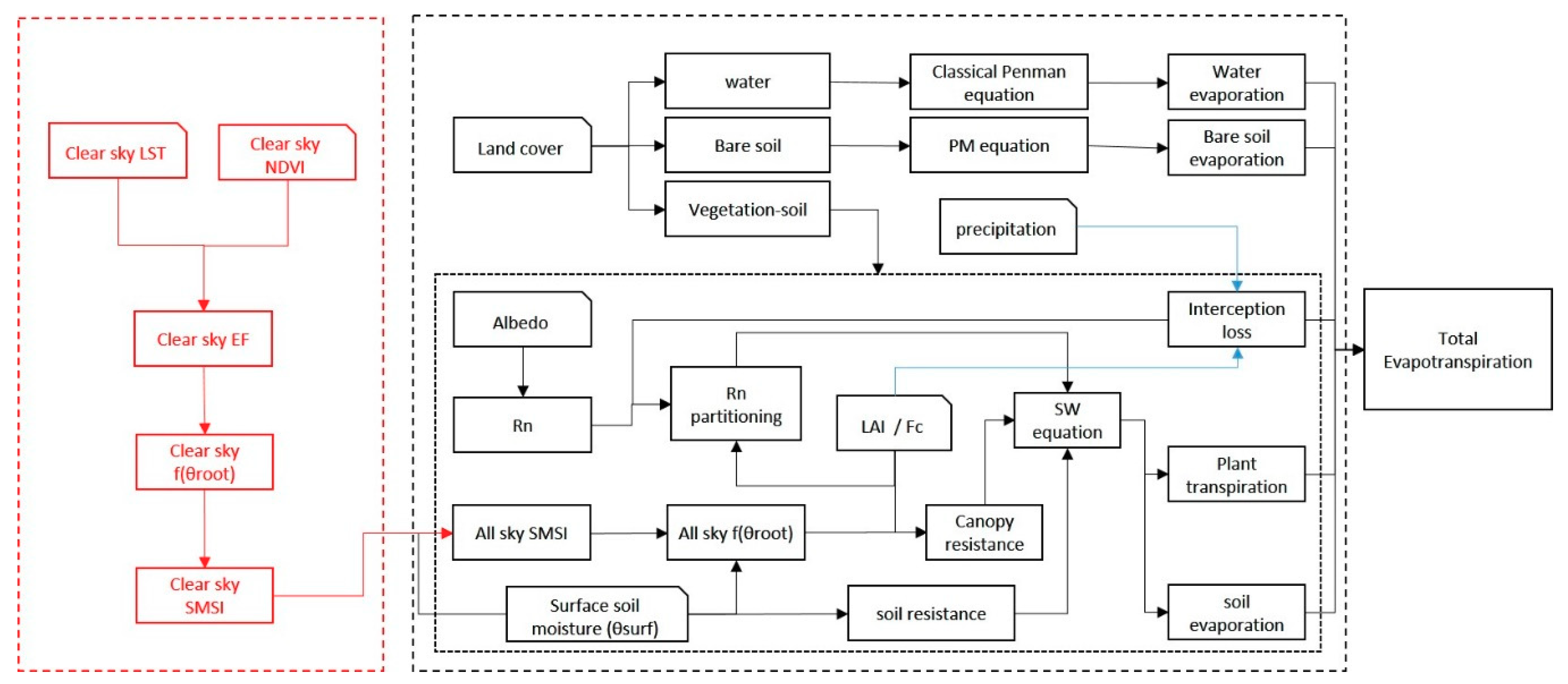
The ET estimation flowchart in current study is shown in Figure 1, and ET from 2001 to 2015 are obtained for the study area.
For bare soil or water pixels, simple PM equation or classical Penman equation is applied to estimate bare soil evaporation and open water evaporation. For the vegetation-soil pixels, detail steps for ET estimation includes:
- (1)
- (2)
- The net radiation is partitioned according to Equations (3)–(5), while during the rainy days in the wet season Rni is estimated by reversing PM equation.
- (3)
- Scatterplot of clear sky LST and NDVI is prepared, and triangle method is applied to retrieve clear sky EF during the Terra and Aqua Moderate Resolution Imaging Spectroradiometer (MODIS) pass time according to Equation (15) in the dry season. The daily EF is assumed to be equal to the EF during the satellite pass time, and daily ET is estimated according to the daily EF and daily available energy;
- (4)
- Daily and f(θroot) of clear days are obtained by reversing Equations (1) and (6), and SMSI is estimated using Equation (12) during these clear days;
- (5)
- SMSI time series is reconstructed by linear interpolation of the SMSI during clear days, hence daily f(θroot) is obtained according to Equation (13) in the dry season; while in the wet season SMSI is taken as constant;
- (6)
- f(θroot) time series is then applied in Equation (6) to estimate daily canopy stomatal resistance, and applied to Equations (1) and (2) to estimate plant transpiration and soil evaporation for all sky conditions.
Finally, these ET components (plant transpiration, soil evaporation, canopy rainfall interception loss, open water evaporation) are summed to total ET. And daily ET in Northeastern Thailand from 2001 to 2015 is achieved in current study.
3. Results
3.1. The Constriant of Soil Moisture on Canopy Resistance and ET
The interpolated daily SMSI for estimating daily canopy resistance was validated over MKL and SKR sites at the dry season. For each site, soil moisture at 10 cm (θ10cm) and 50 cm (θ50cm) depths were available, and surrogated for surface soil moisture and root zone soil moisture. θ50cm is applied in Equation (11) to obtain the constrain of root zone soil moisture on the canopy resistance (f(θ50cm)), which is taken as reference to further compare with f(θroot) by reversing Equations (1) and (6) further, while f(θ50cm)/θ10cm (SMSI50cm) is considered as reference to compare with SMSI.
For the site scale application, when daily latent and sensible heat flux observation is available, mainly in the clear sky, f(θroot) was first retrieved by reversing Equations (1) and (6) (f(θroot)clear day), and SMSI was estimated (SMSIclear day) according to Equation (12). SMSIclear day was interpolated linearly to obtain the daily SMSI (SMSIdaily), and applied in Equation (13) to obtain the estimated f(θroot) (f(θroot)daily). Note that SMSIclear day and f(θroot)clear day are only for the days with valid latent and sensible heat flux observations, while SMSIdaily and f(θroot)daily are temporal continuous during the dry season (Figure 2).
Generally, in the beginning of wet-to-dry episode, the surface soil moisture drops down faster compared to the root zone soil moisture (Figure 2). Several days (e.g., roughly 20 days) from the beginning of dry season in 2003 for MKL site, θroot drop to the level below θmax, and f(θroot) start to decrease, and the decreasing rate is linearly related to the decreasing trend of surface soil moisture. This also lead the uneven decreasing rate of surface soil moisture and f(θroot). However, linear relationship was found between surface soil moisture and f(θroot) during a wet-dry episode, which was defined as the period between two rainy days (Figure 3). Hence, both SMSIdaily and f(θroot)daily could match the temporal variation during the dry season (Figure 2), and both showed low root mean square error (RMSE) and bias with the reference values (Figure 4), indicating the method to parameterize the constrain of soil moisture on canopy resistance based on EF in current study is reasonable.
The uncertainty of SMSI illustrated in Figure 4A will contribute to f(θroot) in Figure 4B. As we can see in the Figure 4, RMSE of 0.31 in SMSI will result in RMSE of 0.09 in f(θroot), mostly because f(θroot) is also regulated by surface soil moisture. This is also shown in Figure 2 that f(θroot)daily is very close to f(θroot), while SMSIdaily bias relative large with SMSIroot. Hence, this interpolation method is considered valid and can be applied to estimate ET in the current study.
3.2. Validating Clear Sky EF by MODIS
The clear sky EF was first derived by LST-VI triangle method, and Figure 5 shows an example of the LST-VI scatter plot and the spatial variation of estimated EF for 20th January, of 2009. Generally, the dry edge and wet edge are well estimated both by Terra and Aqua MODIS. Furthermore, the Terra MODIS-based EF estimates is very close to that of the Aqua MODIS estimates (Figure 6), and both were applied for ET estimation.
To further validate the estimated EF, the estimated EF values over the 6 flux observation sites were extracted to compare with the ground observation, as shown in Figure 7. The observed EF at the satellite pass time is obtained by interpolating the ratio of observed half-hour LE to half-hour available energy to the Terra and Aqua MODIS pass time, while the daily EF is obtained as the ratio between daily LE and available energy. Generally the estimated clear sky EF agree well with observed half-hour and daily EF. Slight difference could be found in terms of RMSE and correlation coefficient, indicating the reasonability of constant EF assumption.
3.3. Comparison of Estimated ET with Flux Tower Observations
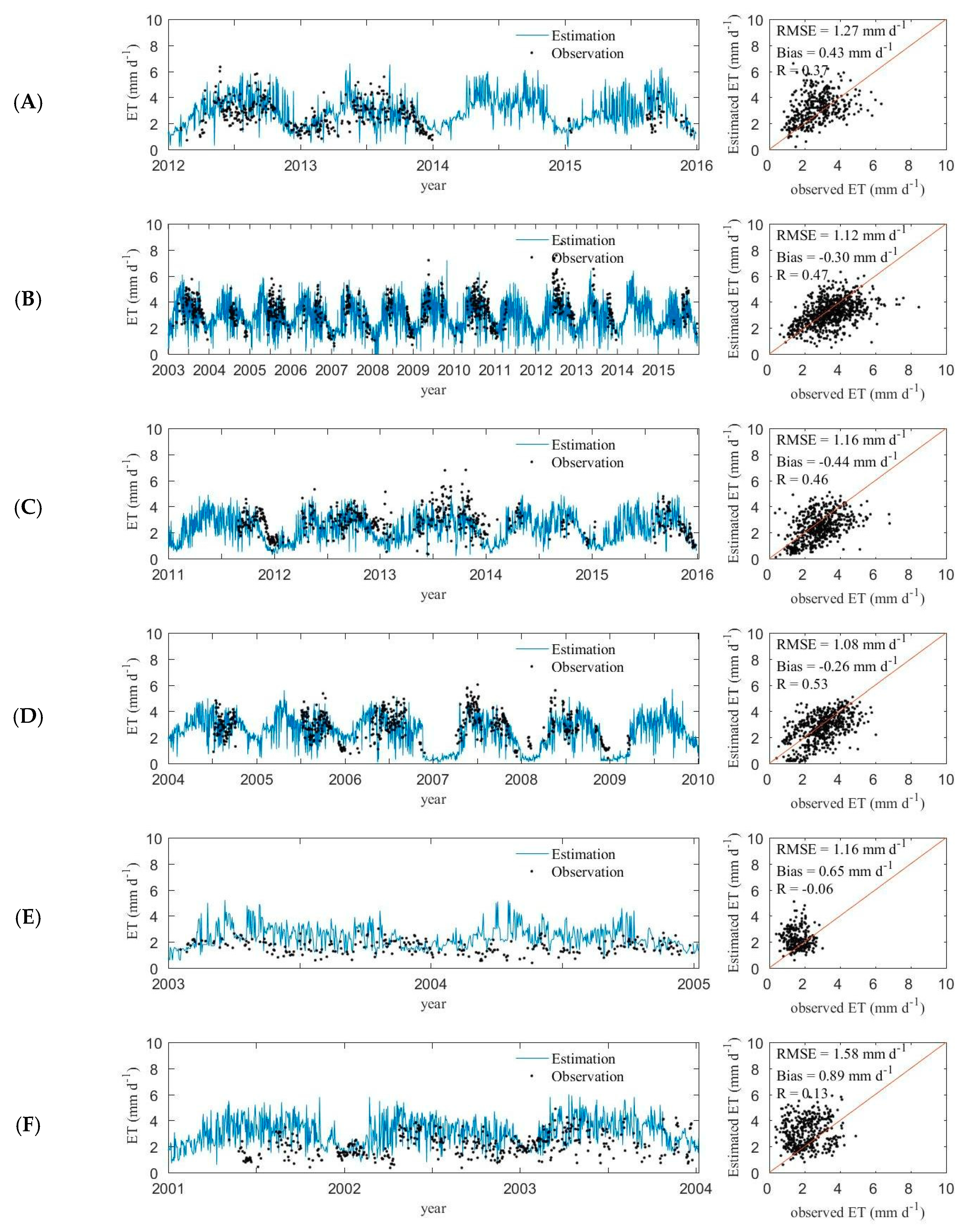
The estimated daily ET agree well with the ground observations, with mean bias range from −0.44 to 0.89 mm d−1 and root mean square error (RMSE) range from 1.08 to 1.58 mm d−1 (Figure 8). The estimated ET could also catch the seasonal variations of ET (Figure 8). These indicate that the estimated ET has relatively good accuracy. Generally, better agreement could be found in the cropland sites than in the forest sites, most likely because significant seasonal variation of ET could be found in cropland while ET in the forest sites showed much less seasonal variation.
Current estimation is compared with the results by original ETMonitor by Hu and Jia (2015) at daily time-step (Table 3). When original ETMonitor by Hu and Jia (2015) was applied, relatively large bias and RMSE could be found, especially for the forest sites. The accuracy is improved by parameter adapting for the forest area, resulting in reduction of RMSE from 1.92–2.12 mm d−1 to 1.16–1.39 mm d−1. It also suggests the necessity to adapt model parameters regionally in the original ETMonitor when applying to different regions to achieve accurate ET estimation. The method developed in current study showed comparable accuracy with the regional adapted ETMonitor, indicating the developed method could be adopted to obtain ET with higher accuracy. This method is operational, and it could reduce the dependence of ground flux observation to calibrate the model parameters.
Current estimation is also compared with the MOD16 ET product at 8-days resolution (Table 4 and Figure 9). Overall, the RMSE of estimated ET (RMSE = 0.97 mm d−1) is much lower than MOD16 ET (RMSE = 1.54 mm d−1) when compared with ground observation. Significant improvement is observed over forest sites (MKL and SKR) where the RMSE are reduced from 2.69 mm d−1 and 1.99 mm d−1 to 1.04 mm d−1 and 1.20 mm d−1.
3.4. Spatial Variation of ET in Northeastern Thailand
Figure 10 shows the spatial variation of estimated annual mean ET, as well as the main ET components including plant transpiration, soil evaporation, and canopy rainfall interception in Northeastern Thailand from 2001 to 2015. The multi-annual mean ET in two largest river basins in this area, Chi and Mun river basins, are 938.8 mm yr−1 and 1023.7 mm yr−1, respectively (Table 5). These two basins are mainly dominant by cropland, which account for 82.16% and 87.45% respectively according MCD12Q1 land cover classification data. Overall, annual precipitation and ET in the Mun river basin is higher than the Chi river basin (Table 5).
Plant transpiration and soil evaporation account for 43.32% and 51.48% of the total ET respectively. The canopy rainfall interception only account for 4.70% of total ET, since this region is mostly covered by low canopy crop, and the area of cropland account for over 80% of the total area, while 80% of the crop is paddy field. The forest only cover roughly 6% of the two basins, mostly located in the Northwest of Chi river basin and Southwest of Mun river basin, where relative high transpiration and interception could be found (Figure 10).
Figure 11 presents the spatial variation of wet season (April to October) and dry season (November to next March) ET in Northeastern Thailand from 2001 to 2015. The wet season ET in Chi and Mun river basins account for 62.30% and 61.27% of annual total ET, while dry season ET in Chi and Mun river basins account for the rest 37.70% and 38.73%.
4. Discussion
The spatially and temporally continuous ET information will advance our knowledge on the mean state and spatial and temporal variability of this significant component of the water cycle, and is highly needed for understanding the interactions between land surface and atmosphere and subsequently improving the water resource management [30]. The LST based surface energy balance method has been proved to provide accurate ET information, but inefficient to produce time series ET due to the cloud [31]. The process-based approach is better for obtaining the spatially and temporally continuous ET products, e.g., the MOD16 ET algorithm. The procedure provided by current study generally combines the advantage of LST-based energy balance method to improve the ET estimation accuracy and the advantage of process model to achieve the spatially and temporally continuous ET estimation, thus it can provide accurate ET estimation, as we showed that the RMSE of estimated ET is low (Figure 8 and Figure 9, Table 3).
It is generally accepted that the RMSE of estimated daily ET range from 1–2 mm d−1 based on satellite forcing, and RMSE of about 50 W m−2 is common reported for latent heat flux (equal to 1.75 mm d−1 ET) [7,10,32]. The RMSE of estimated daily ET in current study range from 1.08 to 1.58 mm d−1, with an averaged RMSE of 1.22 mm d−1, which is less compared to original ETMonitor by Hu and Jia (2015) and MOD16 ET. Generally, MOD16 tend to overestimate forest ET and underestimate cropland ET, which is consistent with several past studies [33,34,35], though not to the same extent as found in this study. Several factors contribute to MOD16 ET uncertainties, e.g., parameterizing soil moisture constrain by meteorological factors (not soil moisture or LST), overestimating environmental stresses on canopy conductance, empirical parameter setting in complementary relationship hypothesis [35,36]. ETMonitor first presented by Hu and Jia (2015) is superior mostly because it is physical robustness, and it considers the impact of soil moisture on ET by introducing the microwave remote sensing-based surface soil moisture and has been demonstrated to be suitable to estimate ET at both regional and global scale [7,37,38]. Although the behavior of original ETMonitor does not meet the expectation in current study, it could be improved by simply adapting its regional parameter to local condition for achieving accurate ET estimation, and is clearly presented by the low RMSE of regional parameter adapted ETMonitor in Table 3. This also highlight the necessity to calibrate parameters to obtain accurate ET estimation when applying locally. Previously, empirical method or soil water balance model was adopted to estimate the root soil moisture based on surface soil moisture, which was further applied to estimate the constrain of soil moisture (f(θroot)) based on fixed soil moisture sensitive parameter. Different from original ETMonitor presented by Hu and Jia (2015), who adopted empirical method to express the constrain of soil moisture on ET, the framework developed in current study provides an operational method to calibrate the algorithm regionally by parameterizing the constrain of soil moisture. The developed framework utilized the LST-VI triangle method to estimate the clear sky EF, which was further applied to estimate SMSI by reversing the canopy resistance equation. It is an operational approach to obtain the canopy resistance parameter for ETMonitor, and it could also be adopted by other ET algorithms.
It has been long recognized that the important variables to determine canopy resistance (or canopy stomatal conductance) include air temperature, humidity, solar radiation, and soil moisture [39,40]. Plants usually open their stomata under wet conditions, which are favorable for plant growth, while when the soil dries stomatal closure limits transpiration to prevent dehydration. Method obtained to express the constrain of soil moisture and climate factors on canopy resistance and evapotranspiration is the key to ensure the accuracy of evapotranspiration algorithms [8,41,42]. The accuracy of ETMonitor estimated ET is also sensitive to the canopy resistance parameter [7]. Different from the traditional calibration method, the developed approach utilized the clear sky EF maps obtained by LST-VI triangle method to retrieve the canopy resistance parameter. One advantage is that it can provide the pixel-to-pixel parameter. The traditional method usually relied on the heavy field work to retrieve the plot scale canopy resistance parameter, which was further applied to regional or global scale according to the land cover map [10]. Thus, traditionally a fixed parameter was usually adopted for a land cover type. However, there exist strong variability in drought tolerance across different plant species, sites, and environmental conditions, which limit the accuracy of global land surface model to simulate the ecosystem response to the decreasing soil moisture, hence much comprehensive calibration method should be addressed [42,43]. The SMSI retrieved by clear sky EF maps obtained by LST-VI triangle method is based on satellite remote sensing image, and can capture the spatial and temporal variation.
LST-VI method is chosen in this study mostly because of its simplicity and accuracy, making it acceptable in the current study (Figure 7). It is also noted that LST-VI method may suffer from domain dependence, and it may impact the accuracy of wet and dry boundary derivation [44]. This spatial-scale effect is common in other anchor-based ET algorithm, e.g., surface energy balance algorithm for land (SEBAL), and caution should be paid when applied to different images in extreme large regions [45,46].
For large regional application, e.g., continents scale, algorithm that is independent of domain size is suggested as alternative. The uncertainty in the input data also contribute to the error of estimated ET in current study. Former study already presented that remote sensing ET algorithms are very sensitive to input variables, e.g., LST, Rn, NDVI, and meteorological variables, depending on which algorithms are adopted [16,32,44,45]. The impact of land cover on ET estimation should also be addressed in ETMonitor, since some sensitive parameters like the minimum stomatal resistance are set according to land cover types. Hence, the uncertainty of land cover classification also contribute to the error in estimated ET.
The linear interpolation of SMSI works well during a wet-dry episode since SMSI generally presents monotonic deceasing trend. However caution should be paid when applying to the frequent rainfall period when the monotonic trend will be disturbed by rainfall. Meanwhile, it is not suitable for those regions where root-zone soil moisture and surface soil moisture are decoupled since the surface soil moisture by satellite remote sensing generally cannot represent the surface wetness condition.
5. Conclusions
ET in Northeastern Thailand was estimated by process-based ETMonitor algorithm based on mainly satellite earth observation datasets. Meanwhile, a new scheme was developed and applied in ETMonitor to take the advantage of LST-based energy balance method. In this scheme, the soil moisture stress index (SMSI) was defined to express the sensitivity of canopy resistance to surface soil moisture, and it was estimated by reversing the canopy resistance equation during the clear sky when EF could be achieved by LST-based energy balance method. The clear sky SMSI was further interpolated to the cloudy days to estimate canopy resistance based on temporal-continuous surface soil moisture data for continuous ET estimation. The estimated daily ET generally agreed well with the flux tower observation with RMSE ranging between 1.08 and 1.58 mm d−1. The RMSE values over the forest sites are considerably lower compared to MOD16 products, indicating its better accuracy.
Author Contributions
C.Z. conceived and designed the study, and wrote the paper; L.J. contributed to the design and revision of the paper; G.H. and J.L. contributed to analyze the clear sky EF estimation and revision of the paper.
Funding
This study is supported by the National Key Research and Development Program of China (Grant no. 2016YFE0117300, no. 2017YFC0405802, and no. 2016YFA0600302), Strategic Priority Research Program of the Chinese Academy of Sciences (Grant no. XDA19080303, and no. XDA19030203), National Natural Science Foundation of China (NSFC) (Grant no. 41801346 and 41501405), National Key Basic Research Program of China (Grant no. 2015CB953702), and 13th Five-Year Plan of Civil Aerospace Technology Advanced Research Projects of China (Grant no. Y7D0070038).
Acknowledgments
We thank Peejush Pani for helping to revise the language. We also thank the reviews by three anonymous reviewers.
Conflicts of Interest
The authors declare no conflict of interest.
References
- Schwalm, C.R.; Williams, C.A.; Schaefer, K. Carbon consequences of global hydrologic change. J. Geophys. Res.-Biogeosci. 2011, 116, 1948–2009. [Google Scholar] [CrossRef]
- Oki, T.; Kanae, S. Global hydrological cycles and world water resources. Science 2006, 313, 1068–1072. [Google Scholar] [CrossRef] [PubMed]
- Zhang, Y.S.; Li, T.; Wang, B.; Wu, G.X. Onset of the summer monsoon over the Indochina Peninsula: Climatology and interannual variations. J. Clim. 2002, 15, 3206–3221. [Google Scholar] [CrossRef]
- Tanaka, N.; Kume, T.; Yoshifuji, N.; Tanaka, K.; Takizawa, H.; Shiraki, K.; Tantasirin, C.; Tangtham, N.; Suzuki, M. A review of evapotranspiration estimates from tropical forests in Thailand and adjacent regions. Agric. For. Meteorol. 2008, 148, 807–819. [Google Scholar] [CrossRef]
- Prabnakorn, S.; Maskey, S.; Suryadi, F.X.; de Fraiture, C. Rice yield in response to climate trends and drought index in the Mun River Basin, Thailand. Sci. Total Environ. 2018, 621, 108–119. [Google Scholar] [CrossRef] [PubMed]
- Bastiaanssen, W.G.M.; Menenti, M.; Feddes, R.A.; Holtslag, A.A.M. A remote sensing surface energy balance algorithm for land (SEBAL)—1. Formulation. J. Hydrol. 1998, 212, 198–212. [Google Scholar] [CrossRef]
- Hu, G.C.; Jia, L. Monitoring of Evapotranspiration in a Semi-Arid Inland River Basin by Combining Microwave and Optical Remote Sensing Observations. Remote Sens. 2015, 7, 3056–3087. [Google Scholar] [CrossRef] [Green Version]
- Bastiaanssen, W.G.M.; Cheema, M.J.M.; Immerzeel, W.W.; Miltenburg, I.J.; Pelgrum, H. Surface energy balance and actual evapotranspiration of the transboundary Indus Basin estimated from satellite measurements and the ETLook model. Water Resour. Res. 2012, 48. [Google Scholar] [CrossRef] [Green Version]
- Miralles, D.G.; Holmes, T.R.H.; De Jeu, R.A.M.; Gash, J.H.; Meesters, A.; Dolman, A.J. Global land-surface evaporation estimated from satellite-based observations. Hydrol. Earth Syst. Sci. 2011, 15, 453–469. [Google Scholar] [CrossRef] [Green Version]
- Mu, Q.Z.; Zhao, M.S.; Running, S.W. Improvements to a MODIS global terrestrial evapotranspiration algorithm. Remote Sens. Environ. 2011, 115, 1781–1800. [Google Scholar] [CrossRef]
- Mu, Q.; Heinsch, F.A.; Zhao, M.; Running, S.W. Development of a global evapotranspiration algorithm based on MODIS and global meteorology data. Remote Sens. Environ. 2007, 111, 519–536. [Google Scholar] [CrossRef]
- Nishida, K.; Nemani, R.R.; Glassy, J.M.; Running, S.W. Development of an evapotranspiration index from aqua/MODIS for monitoring surface moisture status. IEEE Trans. Geosci. Remote Sens. 2003, 41, 493–501. [Google Scholar] [CrossRef]
- Norman, J.M.; Kustas, W.P.; Humes, K.S. Source approach for estimating soil and vegetation energy fluxes in observations of directional radiometric surface-temperature. Agric. For. Meteorol. 1995, 77, 263–293. [Google Scholar] [CrossRef]
- Su, Z. The Surface Energy Balance System (SEBS) for estimation of turbulent heat fluxes. Hydrol. Earth Syst. Sci. 2002, 6, 85–99. [Google Scholar] [CrossRef]
- Zhang, K.; Kimball, J.S.; Nemani, R.R.; Running, S.W. A continuous satellite-derived global record of land surface evapotranspiration from 1983 to 2006. Water Resour. Res. 2010, 46. [Google Scholar] [CrossRef] [Green Version]
- Zheng, C.L.; Wang, Q.; Li, P.H. Coupling SEBAL with a new radiation module and MODIS products for better estimation of evapotranspiration. Hydrol. Sci. J.-J. Des Sci. Hydrol. 2016, 61, 1535–1547. [Google Scholar] [CrossRef]
- Li, Z.L.; Tang, B.H.; Wu, H.; Ren, H.Z.; Yan, G.J.; Wan, Z.M.; Trigo, I.F.; Sobrino, J.A. Satellite-derived land surface temperature: Current status and perspectives. Remote Sens. Environ. 2013, 131, 14–37. [Google Scholar] [CrossRef] [Green Version]
- Jia, L.; Xi, G.; Liu, S.; Huang, C.; Yan, Y.; Liu, G. Regional estimation of daily to annual regional evapotranspiration with MODIS data in the Yellow River Delta wetland. Hydrol. Earth Syst. Sci. 2009, 13, 1775–1787. [Google Scholar] [CrossRef]
- Shuttleworth, W.J.; Wallace, J.S. Evaporation from sparse crops-an energy combination theory. Q. J. R. Meteorol. Soc. 1985, 111, 839–855. [Google Scholar] [CrossRef]
- Jarvis, P.G. The interpretation of the variations in leaf water potential and stomatal conductance found in canopies in the field. Philos. Trans. R. Soc. Lond. B Biol. Sci. 1976, 273, 593–610. [Google Scholar] [CrossRef]
- Allen, R.G.; Pruitt, W.O.; Wright, J.L.; Howell, T.A.; Ventura, F.; Snyder, R.; Itenfisu, D.; Steduto, P.; Berengena, J.; Yrisarry, J.B.; et al. A recommendation on standardized surface resistance for hourly calculation of reference ETO by the FAO56 Penman-Monteith method. Agric. Water Manag. 2006, 81, 1–22. [Google Scholar] [CrossRef]
- Matsumoto, K.; Ohta, T.; Nakai, T.; Kuwada, T.; Daikoku, K.; Iida, S.; Yabuki, H.; Kononov, A.V.; van der Molen, M.K.; Kodama, Y.; et al. Responses of surface conductance to forest environments in the Far East. Agric. For. Meteorol. 2008, 148, 1926–1940. [Google Scholar] [CrossRef]
- Tang, R.L.; Li, Z.L.; Tang, B.H. An application of the T-s-VI triangle method with enhanced edges determination for evapotranspiration estimation from MODIS data in and and semi-arid regions: Implementation and validation. Remote Sens. Environ. 2010, 114, 540–551. [Google Scholar] [CrossRef]
- Stahl, K.; Moore, R.D.; Floyer, J.A.; Asplin, M.G.; McKendry, I.G. Comparison of approaches for spatial interpolation of daily air temperature in a large region with complex topography and highly variable station density. Agric. For. Meteorol. 2006, 139, 224–236. [Google Scholar] [CrossRef]
- Gao, X.J.; Giorgi, F. Increased aridity in the Mediterranean region under greenhouse gas forcing estimated from high resolution simulations with a regional climate model. Glob. Planet. Chang. 2008, 62, 195–209. [Google Scholar] [CrossRef]
- Kim, W.; Miyata, A.; Ashraf, A.; Maruyama, A.; Chidthaisong, A.; Jaikaeo, C.; Komori, D.; Ikoma, E.; Sakurai, G.; Seoh, H.H.; et al. FluxPro as a realtime monitoring and surveilling system for eddy covariance flux measurement. J. Agric. Meteorol. 2015, 71, 32–50. [Google Scholar] [CrossRef] [Green Version]
- Cui, Y.K.; Jia, L. A Modified Gash Model for Estimating Rainfall Interception Loss of Forest Using Remote Sensing Observations at Regional Scale. Water 2014, 6, 993–1012. [Google Scholar] [CrossRef] [Green Version]
- Cui, Y.K.; Jia, L.; Hu, G.C.; Zhou, J. Mapping of Interception Loss of Vegetation in the Heihe River Basin of China Using Remote Sensing Observations. IEEE Geosci. Remote Sens. Lett. 2015, 12, 23–27. [Google Scholar]
- Zheng, C.L.; Jia, L. Global rainfall interception loss derived from multi-source observations. In Proceedings of the 2016 IEEE International Geoscience and Remote Sensing Symposium, Beijing, China, 10–15 July 2016; pp. 3532–3534. [Google Scholar]
- Fisher, J.B.; Tu, K.P.; Baldocchi, D.D. Global estimates of the land-atmosphere water flux based on monthly AVHRR and ISLSCP-II data, validated at 16 FLUXNET sites. Remote Sens. Environ. 2008, 112, 901–919. [Google Scholar] [CrossRef]
- Zhang, Y.Q.; Pena-Arancibia, J.L.; McVicar, T.R.; Chiew, F.H.S.; Vaze, J.; Liu, C.M.; Lu, X.J.; Zheng, H.X.; Wang, Y.P.; Liu, Y.Y.; et al. Multi-decadal trends in global terrestrial evapotranspiration and its components. Sci. Rep. 2016, 6, 19124. [Google Scholar] [CrossRef] [Green Version]
- Michel, D.; Jimenez, C.; Miralles, D.G.; Jung, M.; Hirschi, M.; Ershadi, A.; Martens, B.; McCabe, M.F.; Fisher, J.B.; Mu, Q.; et al. The WACMOS-ET project—Part 1: Tower-scale evaluation of four remote-sensing-based evapotranspiration algorithms. Hydrol. Earth Syst. Sci. 2016, 20, 803–822. [Google Scholar] [CrossRef]
- Hu, G.C.; Jia, L.; Menenti, M. Comparison of MOD16 and LSA-SAF MSG evapotranspiration products over Europe for 2011. Remote Sens. Environ. 2015, 156, 510–526. [Google Scholar] [CrossRef]
- Kim, H.W.; Hwang, K.; Mu, Q.; Lee, S.O.; Choi, M. Validation of MODIS 16 Global Terrestrial Evapotranspiration Products in Various Climates and Land Cover Types in Asia. KSCE J. Civ. Eng. 2012, 16, 229–238. [Google Scholar] [CrossRef]
- Bhattarai, N.; Mallick, K.; Brunsell, N.A.; Sun, G.; Jain, M. Regional evapotranspiration from an image-based implementation of the Surface Temperature Initiated Closure (STIC1.2) model and its validation across an aridity gradient in the conterminous US. Hydrol. Earth Syst. Sci. 2018, 22, 2311–2341. [Google Scholar] [CrossRef] [Green Version]
- Yang, Y.T.; Long, D.; Guan, H.D.; Liang, W.; Simmons, C.; Batelaan, O. Comparison of three dual-source remote sensing evapotranspiration models during the MUSOEXE-12 campaign: Revisit of model physics. Water Resour. Res. 2015, 51, 3145–3165. [Google Scholar] [CrossRef] [Green Version]
- Zheng, C.L.; Jia, L.; Hu, G.; Lu, J.; Wang, K.; Li, Z. Global Evapotranspiration derived By ETMonitor model based on Earth Observations. In Proceedings of the 2016 IEEE International Geoscience and Remote Sensing Symposium, Beijing, China, 10–15 July 2016; pp. 222–225. [Google Scholar]
- Jia, L.; Zheng, C.; Hu, G.; Menenti, M. Evapotranspiration. In Comprehensive Remote Sensing, 2nd ed.; Liang, S., Ed.; Elsevier: Oxford, UK, 2018; Volume 4, pp. 25–50. ISBN 9780128032213. [Google Scholar]
- Klingberg, J.; Engardt, M.; Uddling, J.; Karlsson, P.E.; Pleijel, H. Ozone risk for vegetation in the future climate of Europe based on stomatal ozone uptake calculations. Tellus Ser. A-Dyn. Meteorol. Oceanogr. 2011, 63, 174–187. [Google Scholar] [CrossRef] [Green Version]
- Anav, A.; Proietti, C.; Menut, L.; Carnicelli, S.; De Marco, A.; Paoletti, E. Sensitivity of stomatal conductance to soil moisture: Implications for tropospheric ozone. Atmos. Chem. Phys. 2018, 18, 5747–5763. [Google Scholar] [CrossRef]
- Ershadi, A.; McCabe, M.F.; Evans, J.P.; Wood, E.F. Impact of model structure and parameterization on Penman-Monteith type evaporation models. J. Hydrol. 2015, 525, 521–535. [Google Scholar] [CrossRef]
- Marechaux, I.; Bartlett, M.K.; Sack, L.; Baraloto, C.; Engel, J.; Joetzjer, E.; Chave, J. Drought tolerance as predicted by leaf water potential at turgor loss point varies strongly across species within an Amazonian forest. Funct. Ecol. 2015, 29, 1268–1277. [Google Scholar] [CrossRef]
- Sitch, S.; Huntingford, C.; Gedney, N.; Levy, P.E.; Lomas, M.; Piao, S.L.; Betts, R.; Ciais, P.; Cox, P.; Friedlingstein, P.; et al. Evaluation of the terrestrial carbon cycle, future plant geography and climate-carbon cycle feedbacks using five Dynamic Global Vegetation Models (DGVMs). Glob. Chang. Biol. 2008, 14, 2015–2039. [Google Scholar] [CrossRef]
- Li, Z.S.; Jia, L.; Lu, J. On Uncertainties of the Priestley-Taylor/LST-Fc Feature Space Method to Estimate Evapotranspiration: Case Study in an Arid/Semiarid Region in Northwest China. Remote Sens. 2015, 7, 447–466. [Google Scholar] [CrossRef]
- Long, D.; Singh, V.P.; Li, Z.L. How sensitive is SEBAL to changes in input variables, domain size and satellite sensor? J. Geophys. Res.-Atmos. 2011, 116. [Google Scholar] [CrossRef] [Green Version]
- Tang, R.L.; Li, Z.L.; Chen, K.S.; Jia, Y.Y.; Li, C.R.; Sun, X.M. Spatial-scale effect on the SEBAL model for evapotranspiration estimation using remote sensing data. Agric. For. Meteorol. 2013, 174, 28–42. [Google Scholar] [CrossRef]
Figure 1.
ET estimation flowchart in current study. The left block stands for the land surface temperature (LST)-based method to parameterize the regulation of soil moisture on the ET, while the right block illustrates the interpolation to the cloudy days and the estimation of daily ET.
Figure 1.
ET estimation flowchart in current study. The left block stands for the land surface temperature (LST)-based method to parameterize the regulation of soil moisture on the ET, while the right block illustrates the interpolation to the cloudy days and the estimation of daily ET.

Figure 2.
Time series of soil moisture stress index (SMSI) and f(θroot) at (A) MKL site and (B) SKR site. Soil moisture at 10 cm (θ10cm) and 50 cm (θ50cm) depths are also shown.
Figure 2.
Time series of soil moisture stress index (SMSI) and f(θroot) at (A) MKL site and (B) SKR site. Soil moisture at 10 cm (θ10cm) and 50 cm (θ50cm) depths are also shown.

Figure 3.
The relationship between soil moisture at 10 cm (θ10cm) and f(θ50cm) at (A) MKL site and (B) SKR site at a wet-dry episode. Linear equations are used for fitting(y = 3.42 x − 0.28 with R2 = 0.99 from 27 October 2003 to 5 February 2004 and y = 0.12 x − 0.31 with R2 = 0.20 from 7 February 2004 to 14 March 2004 in MKL, y = 17.87 x − 1.87 with R2 = 0.96 from 3 November 2002 to 8 December 2002 and y = 4.80 x − 0.15 with R2 = 0.97 from 24 December 2002 to 24 February 2003 in SKR).

Figure 4.
Scatterplot comparison of estimated (A) daily SMSI and (B) daily f(θroot) during dry season at MKL and SKR sites.
Figure 4.
Scatterplot comparison of estimated (A) daily SMSI and (B) daily f(θroot) during dry season at MKL and SKR sites.

Figure 5.
Example of LST-VI triangle scatterplot (A,C) and the spatial variation of estimated EF (B,D), by Terra (A,B) and Aqua Moderate Resolution Imaging Spectroradiometer (MODIS) (C,D) at January 20 of 2009. Red line in the LST-VI triangle scatter is the dry edge where =1.26 × Fc, while the blue line is the wet edge where = 1.26.


Figure 6.
Comparison of EF based on Terra and Aqua MODIS on January 20 of 2009. (A) scatter plot of EF based on Terra and Aqua MODIS data; (B) spatial variation of EF difference (EF based on Terra minus that of the Aqua MODIS data).
Figure 6.
Comparison of EF based on Terra and Aqua MODIS on January 20 of 2009. (A) scatter plot of EF based on Terra and Aqua MODIS data; (B) spatial variation of EF difference (EF based on Terra minus that of the Aqua MODIS data).

Figure 7.
Comparison of estimated EF with (A) observed EF at satellite pass time and (B) daily EF obtained by ground observation.
Figure 7.
Comparison of estimated EF with (A) observed EF at satellite pass time and (B) daily EF obtained by ground observation.

Figure 8.
Comparison of ETMonitor estimated daily ET with flux tower based observations in (A) ctt007 site, (B) dtt030 site, (C) prt007 site, (D) pst007 site, (E) MKL site, and (F) SKR site.
Figure 8.
Comparison of ETMonitor estimated daily ET with flux tower based observations in (A) ctt007 site, (B) dtt030 site, (C) prt007 site, (D) pst007 site, (E) MKL site, and (F) SKR site.

Figure 9.
Comparison of (A) ETMonitor estimated 8 days ET in current study and (B) MOD16 ET with ground observed ET.
Figure 9.
Comparison of (A) ETMonitor estimated 8 days ET in current study and (B) MOD16 ET with ground observed ET.

Figure 10.
Spatial variation of (A) plant transpiration, (B) soil evaporation, (C) canopy rainfall interception, and (D) total ET (mm yr-1), in Northeastern Thailand from 2001 to 2015. The boundaries of Chi river basin and Mun river basin are also plotted.
Figure 10.
Spatial variation of (A) plant transpiration, (B) soil evaporation, (C) canopy rainfall interception, and (D) total ET (mm yr-1), in Northeastern Thailand from 2001 to 2015. The boundaries of Chi river basin and Mun river basin are also plotted.

Figure 11.
Spatial variation of (A) wet and (B) dry season ET (mm) in Northeastern Thailand from 2001 to 2015.
Figure 11.
Spatial variation of (A) wet and (B) dry season ET (mm) in Northeastern Thailand from 2001 to 2015.


Table 1.
Main input remote sensing dataset for evapotranspiration (ET) estimation.
| Input Variables | Products Name | Temporal Resolution | Spatial Resolution |
|---|---|---|---|
| Land Cover Types | MCD12Q1 | Yearly | 500 m |
| LST | MOD11A1 & MYD11A1 | Daily | 1 km |
| NDVI | MOD13A2 & MYD13A2 | 8 days | 1 km |
| Albedo | GLASS | 8 days | 1 km |
| LAI | GLASS | 8 days | 1 km |
| Precipitation | CMORPH | Daily | 0.25° |
| Soil Moisture | ESA CCI | Daily | 0.25° |
Table 2.
Flux observation sites information.
| Site ID | Description | Lat (°N) | Lon (°E) | Period | Reference |
|---|---|---|---|---|---|
| ctt007 | Cassava field at Tak | 16.90 | 99.43 | 2012–2015 | [26] |
| dtt030 | Diverse land surface at Tak | 16.94 | 99.43 | 2003–2015 | [26] |
| prt007 | Paddy at Rachaburi | 13.58 | 99.51 | 2011–2013 | [26] |
| pst007 | Paddy at Sukhothai | 17.06 | 99.70 | 2004–2009 | [26] |
| MKL | Forest at Sakaerat | 14.59 | 98.84 | 2003–2004 | [4] |
| SKR | Forest at Mae Klong | 14.49 | 101.92 | 2001–2003 | [4] |
Table 3.
Comparison of estimated daily ET by current improved ETMonitor and original ETMonitor by Hu and Jia (2015) with ground observed ET. Values in the baskets represent the results after adapting the parameters by Hu and Jia (2015) to the humid climate in Northeast Thailand.
Table 3.
Comparison of estimated daily ET by current improved ETMonitor and original ETMonitor by Hu and Jia (2015) with ground observed ET. Values in the baskets represent the results after adapting the parameters by Hu and Jia (2015) to the humid climate in Northeast Thailand.
| Site ID | ETMonitor by Hu and Jia (2015) | Current Study Estimation | ||||
|---|---|---|---|---|---|---|
| R | Bias (mm d−1) | RMSE (mm d−1) | R | Bias (mm d−1) | RMSE (mm d−1) | |
| ctt007 | 0.48 | 0.02 | 1.06 | 0.37 | 0.43 | 1.27 |
| dtt030 | 0.62 (0.45) | −1.70 (−0.77) | 1.95 (1.25) | 0.47 | −0.3 | 1.12 |
| prt007 | 0.45 | −0.37 | 1.21 | 0.46 | −0.44 | 1.16 |
| pst007 | 0.51 | −0.33 | 1.12 | 0.53 | −0.26 | 1.08 |
| MKL | −0.02 (0.00) | 1.59 (0.68) | 1.92 (1.16) | −0.06 | 0.65 | 1.16 |
| SKR | 0.14 (0.07) | 1.67 (0.44) | 2.12 (1.39) | 0.13 | 0.89 | 1.58 |
Table 4.
Comparison of ETMonitor estimated 8 days ET and MOD16 8 days ET with ground observed ET.
| Site ID | ETMonitor 8-Days ET | MOD16 8-Days ET | ||||
|---|---|---|---|---|---|---|
| R | Bias (mm d−1) | RMSE (mm d−1) | R | Bias (mm d−1) | RMSE (mm d−1) | |
| ctt007 | 0.59 | 0.44 | 0.94 | 0.30 | 0.36 | 1.19 |
| dtt030 | 0.59 | −0.31 | 0.92 | 0.50 | −0.09 | 0.98 |
| prt007 | 0.65 | −0.37 | 0.82 | 0.23 | −0.03 | 0.99 |
| pst007 | 0.63 | −0.45 | 0.97 | 0.59 | −0.55 | 1.12 |
| MKL | 0.07 | 0.75 | 1.04 | 0.48 | 2.58 | 2.69 |
| SKR | 0.30 | 0.78 | 1.20 | 0.42 | 1.82 | 1.99 |
Table 5.
Statistic information of Chi and Mun river basins.
| Basin Area (× 103 km2) | Annual Precipitation (mm yr−1) | Annual ET (mm yr−1) | Cropland Coverage (%) | Forest Coverage (%) | |
|---|---|---|---|---|---|
| Chi river basin | 40.58 | 1269.52 | 938.80 | 82.16 | 5.56 |
| Mun river basin | 71.06 | 1374.50 | 1023.70 | 87.45 | 6.56 |
© 2019 by the authors. Licensee MDPI, Basel, Switzerland. This article is an open access article distributed under the terms and conditions of the Creative Commons Attribution (CC BY) license (http://creativecommons.org/licenses/by/4.0/).
Share and Cite
MDPI and ACS Style
Zheng, C.; Jia, L.; Hu, G.; Lu, J. Earth Observations-Based Evapotranspiration in Northeastern Thailand. Remote Sens. 2019, 11, 138. https://doi.org/10.3390/rs11020138
AMA Style
Zheng C, Jia L, Hu G, Lu J. Earth Observations-Based Evapotranspiration in Northeastern Thailand. Remote Sensing. 2019; 11(2):138. https://doi.org/10.3390/rs11020138
Chicago/Turabian StyleZheng, Chaolei, Li Jia, Guangcheng Hu, and Jing Lu. 2019. "Earth Observations-Based Evapotranspiration in Northeastern Thailand" Remote Sensing 11, no. 2: 138. https://doi.org/10.3390/rs11020138
Note that from the first issue of 2016, this journal uses article numbers instead of page numbers. See further details here.