A Modeling Framework for Deriving Daily Time Series of Evapotranspiration Maps Using a Surface Energy Balance Model


1
Department of Biosystems & Agricultural Engineering, Oklahoma State University, Stillwater, OK 74078, USA
2
USDA-ARS Grazinglands Research Laboratory, El Reno, OK 73036, USA
3
Formation Environmental LLC, Sacramento, CA 95816, USA
*
Author to whom correspondence should be addressed.
Remote Sens. 2019, 11(5), 508; https://doi.org/10.3390/rs11050508
Submission received: 11 January 2019
/
Revised: 25 February 2019
/
Accepted: 26 February 2019
/
Published: 2 March 2019
(This article belongs to the Special Issue Remote Sensing of Evapotranspiration (ET))
Abstract
:Surface energy balance models have been one of the most widely used approaches to estimate spatially distributed evapotranspiration (ET) at varying landscape scales. However, more research is required to develop and test an operational framework that can address all challenges related to processing and gap filling of non-continuous satellite data to generate time series of ET at regional scale. In this study, an automated modeling framework was developed to construct daily time series of ET maps using MODIS imagery and the Surface Energy Balance System model. The ET estimates generated from this modeling framework were validated against observations of three eddy-covariance towers in Oklahoma, United States during a two-year period at each site. The modeling framework overestimated ET but captured its spatial and temporal variability. The overall performance was good with mean bias errors less than 30 W m−2 and root mean square errors less than 50 W m−2. The model was then applied for a 14-year period (2001–2014) to study ET variations across Oklahoma. The statewide annual ET varied from 841 to 1100 mm yr−1, with an average of 994 mm yr−1. The results were also analyzed to estimate the ratio of estimated ET to reference ET, which is an indicator of water scarcity. The potential applications and challenges of the ET modeling framework are discussed and the future direction for the improvement and development of similar automated approaches are highlighted.
1. Introduction
Time series of remotely sensed evapotranspiration (ET) maps have extensive applications in agricultural, hydrological and environmental studies as they capture the spatiotemporal variability of vegetation consumptive use from field to continental scales. For example, spatial ET data have been used in agriculture sector for water right regulation, planning and monitoring [1], assessing irrigation and drainage performance [2,3,4], closing water balance at irrigation scheme levels [5] and managing agricultural water resources [6,7,8]. Recent studies have shown that remotely sensed ET can be used effectively for monitoring agricultural droughts [9,10,11] with the future potential of improving the performance of ET-integrated agricultural drought indices [12]. ET maps have been also used in assessing crop water productivity [13,14,15] and crop yield analysis [16,17].
Numerous studies have demonstrated the use of time series ET maps for ecological applications, such as capturing the progress of vegetation and wetland restoration [18], assessing the vulnerability of forest to fire and drought [19] and accounting water use from riparian vegetation and invasive species [20,21,22,23]. Remote sensing-based ET products have also been applied in improving the performances of hydrological models [24,25,26] and for climate studies to capture water feedbacks associated with seasonal cycles and soil moisture deficit at regional scales [27].
Among different approaches developed for mapping ET, the surface energy balance (SEB) approach has been widely used to acquire distributed ET at varying geographical scales [28,29,30,31]. Numerous SEB models have been proposed, including but not limited to Surface Energy Balance Index (SEBI) [32], Two-Source Energy Balance (TSEB) [33,34], Surface Energy Balance Algorithm for Land (SEBAL) [35], Simplified Surface Energy Balance Index (S-SEBI) [36], Surface Energy Balance System (SEBS) [37], Mapping Evapotranspiration at high Resolution with Internalized Calibration (METRIC) [38], Atmosphere-Land Exchange Inverse (ALEXI) [39], Regional ET Estimation Model (REEM) [40], Remote Sensing Evapotranspiration model (ReSET) [41], Operational Simplified Surface Energy Balance (SSEBop) [42] and Hybrid Dual-Source Scheme and Surface Energy Framework-Based Evapotranspiration Model (HTEM) [43]. Some of these models such as SEBAL and METRIC use manual selection of extreme pixels to compute sensible heat flux, which could result in variations in estimated ET [44] and may add uncertainty and errors based on the user’s experience [45]. Other models such as TSEB, SEBS and SSEBop do not require human intervention so that the associated uncertainties are minimized. The selection of the SEB model and the quality of input data are likely key factors to determine the accuracy of modeled ET [46].
Developing time series of ET maps requires complex, multi-step analyses to deal with issues associated with pre-processing of remote sensing data and post-processing of resulting ET products. The choice of the SEB model and satellite data could vary depending on intended applications of ET maps, availability and requirements of input data and availability of resources (time, money and expertise) to run the model. In general, the SEB-based ET estimation process can be divided into six steps: (i) collation of remotely sensed and ground-based input data, (ii) quality assessment of collected datasets and preparation of all necessary inputs for the selected SEB model, (iii) running the SEB model (including all modules and algorithms) to obtain the instantaneous ET at the time of satellite overpass, (iv) extrapolation of instantaneous ET to daily estimates, (v) filling the gaps due to cloud coverage over a portion of the map and (vi) interpolation of daily ET between image acquisition dates to obtain ET for longer time scales.
The first two steps are performed to ensure the quality of input data, a critical requirement for any remote sensing data analysis. A thorough QA/QC procedure for weather data as presented in [47,48] is necessary as the accuracy of final product depends on the quality of these datasets. The quality assurance of weather dataset is even more critical in case of SEB models as they are sensitive to weather parameters. For example, Webster et al. [49] found air temperature and wind speed as influential inputs for HTEM and SEBS models, whereas, S-SEBI was less sensitive to meteorological inputs.
For small-scale applications with similar climatic conditions, weather data from a single ground station are usually used as input in most SEB models. However, for regional applications with varying climatic conditions, distributed datasets are required. Several recent studies [50,51] have applied gridded weather datasets for mapping daily ET due to the ease of their application for regional studies. However, users need to confirm the integrity of the datasets before processing the SEB model. A study [52] found overestimation of reference ET due to biases in air temperature and wind speed in the widely used reanalysis data—North American Land Data Assimilation System when compared to reference ET estimates from the Texas High Plains ET Network [53]. The study recommended using weather station datasets within agricultural settings, whenever possible, for precise applications of time series ET information such as in irrigation scheduling. A few studies have explored the applicability of developing distributed weather data from the point measurements of a network of ground stations to account for the spatial variability of weather parameters [54].
The third step is to run the selected SEB model, which involves several sub-models to solve the SEB equation as shown in Equation (1).
where LE is latent heat flux, Rn is net radiation, G is soil heat flux and H is sensible heat flux. All parameters are in units of W m−2. Based on the sensible heat flux computation approach, SEB models can be categorized into single-source and two-source models. The sensible heat fluxes for soil and vegetation are computed separately in two-source models, while a single value for each pixel is computed in single-source models. Each approach has its own advantages and caveats. In theory, two-source models could provide more accurate ET over sparse vegetation as they close the energy balance separately for soil and vegetation. Timmermans et al. [44] found better accuracy from a TSEB model compared to SEBS across sparsely vegetated grasslands in the Southern Great Plains. Kustas et al. [55] reported that two-source performed better in sub-humid tallgrass prairie, whereas greater accuracy was found for a single-source model in semiarid rangeland.
As mentioned before, some single-source models require an additional step in running the model, which involves the manual selection of extreme hot and cold pixels by user. To remove the subjectivity in the selection of extreme pixels in SEBAL, Long et al. [56] introduced a trapezoidal approach to define boundary conditions for the selection of these pixels based on the relationship between vegetation fraction and surface temperature. Automated approaches have been proposed in [57,58,59] to replace human intervention. Alternative approaches are also applied by [60,61] to estimate ET from a cold pixel as a function of normalized difference vegetation index when an ideal cold pixel is difficult to find within a satellite image.
The fourth step is to extrapolate the instantaneous ET to daily values. Evaporative fraction (Λ) [35,37,62,63] and ETrF (fraction of reference ET) [38,64] are the common methods to obtain daily ET. Both of these methods assume the instantaneous Λ or ETrF is the same as the daily Λ or ETrF. However, a study [65] reported that this assumption was not satisfied when the fractional vegetation cover was close to a maximum. In the Texas Panhandle, Colaizzi et al. [66] found a better agreement of ETrF method for cropland and Λ method for bare soil when compared with lysimeter measurements. Chavez et al. [67] evaluated six extrapolation approaches on corn and soybean fields and found smaller error from Λ method when compared with eddy covariance measurements. Another study [68] found Λ method advantageous during several water stress events, whereas ETrF approach performed better under advective conditions [38,64], which could be significant in arid environments.
The fifth step is to fill the gaps caused by cloud coverage over a portion of the daily ET maps. One approach is to apply linear interpolation of nearest reliable values within an image [50]. This method is suitable when the nearest pixels are under the same land cover as that of missing pixels. However, it may not be appropriate when the area with data gap is large and encompasses heterogeneous terrain. Another approach includes the use of time-weighted interpolation of preceding and following images [69]. This method adjusts the vegetation development using normalized difference vegetation index (NDVI) across vegetated areas and residual soil moisture differences for the areas with bare soil surface. Anderson et al. [39] applied the available water for the root zone and soil surface layer to fill the gaps. The available water for the clear and cloudy days is used to estimate the daily water depletion due to ET from the root zone and soil surface layer and the fraction of available water is used to fill the gaps.
The final step is the interpolation of ET maps between consecutive satellite overpass dates to construct daily ET time series. Several interpolation and data-fusion approaches have been implemented for this purpose. A common approach is to apply linear interpolation of Λ or ETrF images between consecutive satellite overpass dates [70]. Another approach is to apply a curvilinear function using more than two Λ or ETrF images. For example, at least one cloud-free image for each month was used for spline interpolation within METRIC to obtain monthly and seasonal ET [38,71,72]. Singh et al. [70] evaluated the performance of several interpolation methods and found no significant difference in seasonal ET among cubic spline, fixed ETrF and linear interpolations. A backward-average iterative approach has been also proposed to estimate ET in between Landsat overpass dates [73].
While numerous studies have been conducted to address the issues related to specific steps involved in generating remotely sensed ET time series based on SEB models, only a few have focused on developing automated modeling frameworks, covering all hierarchical steps mentioned above. Such modeling frameworks, if validated, could have significant value in providing end-users with daily ET time series for practical applications in improving land and water management. Furthermore, a comprehensive and detailed documentation of the entire process of deriving daily ET maps at regional scales could be a useful resource to potential end-users who currently need to understand and select appropriate approaches for each of the six steps from many sources. Developing and documenting a comprehensive framework that generates complete ET time series from raw input data enables potential users outside the research community to utilize this framework for making more informed decisions and policies. The main goal of this study was to develop and document a modeling framework to construct daily time series of ET maps for the entire state of Oklahoma, USA. The performance of this framework was also evaluated by comparing its results with ET estimates of flux towers in Oklahoma. Finally, long-term variations in ET across Oklahoma were investigated.
2. Materials and Methods
2.1. Study Area
The study area covered the entire state of Oklahoma, USA, with an area of about 181,200 km2 (Figure 1). Oklahoma Climate is classified as humid subtropical at most parts of the state and cold semi-arid at far west [74]. The state has nine climate divisions (CD) delineated based on precipitation and temperature gradients. The normal (1981–2010) annual precipitation is about 925 mm yr−1, with significant spatial variation across CDs. While southeast (CD9) receives the largest amount of 1301 mm yr−1 on average, the Panhandle (CD1) holds the smallest record of 520 mm yr−1. The normal annual mean air temperature is 15.6 °C, with July and January being the hottest and coldest months, respectively. The southcentral (CD8) has the maximum mean annual temperature of 16.7 °C, whereas the Panhandle region has the minimum value at 13.6 °C. The top two land cover categories in Oklahoma are grassland (36.4%) and pastureland (11.3%) [75]. The elevation varies between 88 m above mean sea level at the southeast border with Arkansas and 1516 m at far-west border with New Mexico.
2.2. Modeling Framework
The modeling framework was designed to use daily images from the MODIS Terra satellite as input data. The single-source SEBS model [37] was selected as the SEB model for estimating energy fluxes. The main reason for the selection of SEBS over other SEB models was its applicability over large areas with heterogeneous surfaces [31]. In addition, this model does not require intermittent human intervention, which facilitates the automation process. A graphical illustration of the proposed framework is shown in Figure 2, followed by detailed explanation of specific approaches selected for each of the six computational steps mentioned before.
2.2.1. Step 1: Collation of Input Data
The daily surface reflectance (MOD09GA, [76]), daily land surface temperature (LST) and emissivity (MDO11A1, [77]) data were downloaded from the US Geological Survey Land Processes Distributed Active Archive Center (https://lpdaac.usgs.gov/). Ground-based meteorological data included hourly air temperature, relative humidity, incoming shortwave solar radiation, wind speed and atmospheric pressure. These data were obtained from the Oklahoma Mesonet [78,79] weather stations installed across the state (Figure 1). The Oklahoma Mesonet is a world-class environmental monitoring network (https://www.mesonet.org/) consisting of 120 active stations with at least one station at each of the 77 counties in Oklahoma.
2.2.2. Step 2: Quality Assessment and Preparation of Inputs
The initial quality assessment of suitable MODIS images was based on cloud coverage. Images with less than 10% cloud cover were selected for further processing. Hence, any day when the cloud coverage was above 10% was assumed as a day with missing remotely sensed data. When the period of missing imagery was more than 10 consecutive days, images with less than 15% cloud cover were also included as acceptable quality. Then, cloud-covered pixels in each selected image were masked by applying a threshold of LST smaller than 250 K. These steps were repeated for all selected reflectance, LST and emissivity images. Since a single MODIS image tile was not sufficient to cover the entire state of Oklahoma, two image tiles (h09v05 and h10v05) were merged.
The quality assessment of each weather variables was performed as described in [47,48]. The solar radiation was checked against the upper limit under clear sky condition. Daily average temperature was compared against the average extreme temperatures to ensure the difference between them was within the acceptable range (2 °C) [48]. The quality of wind speed was maintained by considering gust factor threshold of more than 1. Relative humidity data were considered when the values were less than 100%. The missing weather data were filled by an average value of that parameter from four nearest Mesonet stations. Hourly alfalfa reference ET (ETr) [48] was then computed at each station during the study period using the Bushland ET Calculator [80]. Daily ETr estimates were obtained by summing 24-hour ETr values. To incorporate the weather variability between the weather stations, spatial input data were generated by applying inverse distance weighted interpolation for all weather variables, including hourly and daily ETr. As mentioned in the previous section, the Oklahoma Mesonet is a densely distributed weather station network, with about 1510 km2 per station. This is a significantly finer spatial resolution than the 5000 km2 per station value recommended by the World Meteorological Organization for evaporation stations on interior plains [81]. Hence, the adjustment of meteorological parameters with elevation was not considered during interpolation.
2.2.3. Step 3: The SEB Model
As mentioned before, the Surface Energy Balance System (SEBS) model of [37] was selected as the SEB model in the present study. However, other SEB models such as those reviewed in the Introduction section can be used in this step based on user resources, availability of input data and desired accuracy. Like other SEB models, SEBS estimates the latent heat flux (LE) as a residual of the land surface energy balance as shown in Equation (1). The Rn was calculated by applying the surface radiation balance equation:
where RS is incoming shortwave solar radiation, α is surface albedo (dimensionless) estimated following [82], εa and εs are emissivities (dimensionless) of atmosphere and surface, estimated following [83,84], respectively. σ is the Stefan-Boltzmann constant (5.67 × 10⁻⁸ W m−2 K−4), TA is air temperature (K) and Ts is the surface temperature (K), estimated as a ratio of brightness temperature to εs−0.25. The G was estimated by applying the relationship developed by [35]:
where c1 and c2 are calibration coefficients and were considered as 0.24 and 0.46, respectively.
SEBS uses similarity theories to estimate H: the bulk atmospheric similarity (BAS) theory for atmospheric boundary layer (ABL) scaling [85] and the Monin-Obukhov similarity (MOS) for atmospheric surface layer (ASL) scaling [86]. The ABL is a part of the atmosphere that is directly impacted by earth’s surface and responds to surface forcing with a timescale of an hour or less, whereas ASL is usually the bottom 10% of ABL [37]. During unstable conditions, an appropriate atmospheric (BAS or MOS) scaling is determined as presented in [83]. For stable conditions, functions given by [83,87] are used for ABL and ASL scaling, respectively. In the ASL, the similarity relationships for mean wind speed (u) and the difference between potential temperature profiles are derived using the MOS theory as:
where u* is the friction velocity (m s−1), k is the von Karman’s constant (0.41), z is the height above the surface (m), d0 is the zero plane displacement height (m), z0m is the roughness height for momentum transfer (m) estimated using an empirical relationship with NDVI [88], z0h is roughness height for heat transfer (m), θ0 is the potential air temperature at surface (K), θa is the potential air temperature at z (K), θv is the potential virtual temperature near the surface (K), ρa is the air density (kg m−3), Cp is the specific heat capacity of air (1013 J kg−1 K−1) and g is the gravitational acceleration (9.8 m s−2). ψm and ψh are the stability correction functions for momentum and sensible heat transfer, respectively and L is the Monin–Obukhov length (m).
The scalar roughness height for heat transfer, z0h, is an important parameter to regulate the heat transfer between the land surface and the atmosphere and estimated as:
where kB−1 is the Stanton number, a dimensionless heat transfer coefficient, estimated using a formulation from [89] as:
The heat transfer coefficient in Equation (8) was formulated to account for three different land surface conditions. The first term follows the Choudhury and Monteith [90] model for full canopy, the second term accounts for the interaction between the vegetation and soil surface and the third term is for the bare soil surface given [83]. In this equation, fc and fs are canopy and soil fraction coverage, respectively, Cd is the drag coefficient for the foliage with a value of 0.2; Ct and Ct* are the heat transfer coefficients of the leaf and soil, respectively. The value of Ct was taken as 0.03 and Ct* was computed from Prandtl number and roughness Reynolds number (Re*) [37]. The u(h) in Equation (8) is the horizontal wind speed at the canopy top (m s−1) and h is canopy height (m) estimated as a ratio of z0m to 0.136 [37]. The nec (within-canopy wind speed profile extinction coefficient) and Brutsaert term kBS−1 (for bare soil surface) were calculated as:
where LAI is the leaf area index and estimated as a functional relation with NDVI [91].
SEBS requires estimation of H for dry (Hdry) and wet (Hwet) boundary conditions. Under dry conditions, the Hdry is equivalent to the available energy (Rn − G) as there is no evaporation due to the limitation of water availability and Hwet is calculated using the Penman-Monteith equation [92,93]. After computing H for boundary conditions, the relative evaporative fraction (Λr), the evaporative fraction (Λ) and ET are estimated. The steps and explanation are detailed in [37]
2.2.4. Step 4: Extrapolation of Instantaneous to Daily ET
The SEBS uses the Λ approach for scaling instantaneous ET to daily ET, assuming the Λ at the time of overpass is equal to the daily Λ. In this study, a modified approach was implemented where either Λ or ETrF is used for extrapolation of each pixel based on its NDVI value as shown in Equation (15).
where ETinst and ETr are the actual and reference ET at the hour of satellite overpass (mm h−1), λ is the latent heat of vaporization (~2.45 MJ kg−1). ETr24 is the daily reference ET and ET24 is the daily actual ET (mm d−1). This modification was made to take the advantage of Λ and ETrF approach to better represent the water limited and energy limited conditions, respectively. The ETrF was estimated as a ratio of ET obtained from Step 3 to reference ET at the satellite overpass time (MODIS Terra satellite overpass local time around 10:30 AM).
2.2.5. Step 5: Filling the Gaps Due to Cloud Cover
Data-gaps due to cloud cover is a common issue in all space-borne satellites. In this study, crop coefficient (Kc) was used to fill the data-gaps. The Kc maps were created for all images as the ratio of ET24 and respective daily ETr. To fill the Kc of a cloud covered (missing) pixel for a specific image date, the Kc value of the same pixel from the preceding image date was first used. If the same pixel was missing in the preceding image, the Kc value was obtained from the next Kc map. The latter step was repeated if the next day was missing until a date was found with a Kc value estimated for the same pixel. This interpolation method was suitable to fill the data gaps as most of the selected images were less than 10 days apart during the crop growing season (April to October).
2.2.6. Step 6: ET for Longer Periods
After filling the data gaps in daily ET maps due to clouds, the ET maps needed to be created for days when the cloud coverage was more than 10% (or 15%) and thus no input imagery was available. To fill these gaps, the average Kc of the preceding and following images closest to the image date of interest was used. The Kc images were then multiplied with respective daily ETr to obtain complete time series of daily ET maps. Construction of weekly, monthly, seasonal and annual ET maps was accomplished by summation of daily ET maps over corresponding periods. The processing of all steps was executed in Python language within ArcGIS environment.
2.3. Comparison with Flux Tower Data
Daily ET time series from the modeling framework explained above were compared against observed ET from three flux towers: US-ARc (35.5464 N, 98.0400 W), US-ARb (35.5497 N, 98.0402 W) [94] and US-AR2 (36.6358 N, 99.5975 W) [95]. The US-ARc and US-ARb were located close to each other over native grassland in central Oklahoma. The US-AR2 was located over planted switchgrass in northwest Oklahoma. The 30-minute flux data from the towers were downloaded from the AmeriFlux data archive (http://ameriflux.lbl.gov/) for years 2005 and 2006 for US-ARc and US-ARb sites and years 2010 and 2011 for the US-AR2 site. The flux tower data usually have the issue with energy balance closure, therefore, the closure error was corrected by maintaining constant Bowen-ratio following [96]. The corrected 30-min data were averaged to obtain daily data. The daily observed ET was then compared with the average values of 3 × 3 pixels (~1390 m × 1390 m) from the SEBS ET at the flux tower locations. It should be noted that the three flux towers used for validating the performance of the modeling framework in this study represent only two land covers (native and managed grassland). Hence, the performance of the framework may be different from what is documented here over different types of land covers not included in the present analysis.
For statistical analysis, correlation coefficient (r), the coefficient of determination (R2), mean absolute error (MAE), mean bias error (MBE) and root mean square error (RMSE) were used:
where FT-ET is the observed flux tower daily ET and SEBS-ET is the estimated daily ET from the SEBS model.
2.4. Application of the Modeling Framework
After evaluating the accuracy of the modeling framework, it was used to estimate annual ET maps over the entire state of Oklahoma, as well as its nine climate divisions (CD), during the 2001–2014 period. The annual ET were also compared with publicly available MOD16 ET dataset [97,98] over the same period, which covers the most recent drought episode of 2011–2014. The degree of water availability for each pixel and CD within Oklahoma was assessed by estimating the ratio of annual ET from the modeling framework and the reference ET. This ratio is an indication of the portion of the atmospheric demand that is supplied at each pixel and CD. Areas with smaller ratios represent water scarcity since the actual ET from the model is far from the potential limits of ET. The information on annual ET variations and water availability across Oklahoma can assist state water managers with making critical decisions based on long-term objective data from the implemented framework. As mentioned before, the validation dataset only represented native and managed grassland. About half (47%) of all lands in Oklahoma are under rangeland and grassland. With winter wheat being the most dominant crop, the majority of croplands have similar canopy characteristics. Nevertheless, the lack of representation of other land covers (e.g., 21% of forest in Oklahoma) should be considered in applications and interpretations of the results of the modeling framework.
3. Results and Discussion
3.1. Comparison with Flux Tower Data
The comparison with flux tower data showed good agreement between daily SEBS-ET and FT-ET. The modeling approach captured the spatial and temporal variations in ET. However, the model overestimated ET at all sites and years (Figure 3), with average MBE of 20.1 W m−2. The range of MBE was between 1.7 W m−2 at US-AR2 in 2011 and 29.3 W m−2 at US-ARb in 2006 (Table 1). The mean MAE and RMSE were 33.0 W m−2 and 42.7 W m−2, respectively. The correlation coefficients varied from 0.61 to 0.81 and R2 from 0.37 to 0.66.
The errors in the ET estimates of the modeling framework are due to errors generated in each of the six steps outlined in previous section. A major step for error introduction is step three, that is, the surface energy balance model. Previous studies have reported uncertain characterization of kB−1 in water limited environments [99,100,101] and in low vegetation cover conditions [102]. Overestimating kB−1 under these conditions would lead to overestimating z0h, underestimating H and consequently overestimating ET [99]. The overestimation errors observed in this study were within the range of errors in previous studies when using MODIS as the input imagery to SEBS model. For example, [103] reported ET overestimation with MBE of 6.1 W m−2; [104] found MBE of 20.1 W m−2 and RMSE of 34.7 W m−2; [105] reported MBE of 144.9 W m−2 when comparing SEBS-ET from cropland and grassland with flux tower estimates; [106] found overall MBE of 31 W m−2 and RMSE of 76 W m−2; and, [107] reported MBE of 95.1 W m−2 and RMSE of 122.2 W m−2 across several land covers and climatic conditions. While several studies have reported overestimation error from SEBS, the mean absolute error from the current study was smaller than the threshold of 50 W m−2 suggested by [108].
Errors in other steps of the framework can contribute to biases in final ET estimates. A common source of error in estimating ET from satellite imagery is due to cloud contamination. A thin layer of cloud or a shaded area due to cloud presence over nearby pixels can result in underestimation of LST and consequently, overestimation of ET. In practical applications, it is impossible to remove all these contaminated pixels from the entire image even after applying the LST thresholds during quality control. In this study, there were days with underestimated LST due to cloud presence. For example, the LST at the flux tower pixel area dropped by 10.6 K from Day of Year (DOY) 113 to 114, while both DOYs were identified as cloud-free and no precipitation was recorded. The instantaneous TA increased by 3.2 K over the same period. The smaller LST on DOY 114 affected ET estimation for this day and the following days until another cloud-free image was obtained for DOY 117 (Figure 3a).
A sensitivity analysis study [109] on SEBS model reported LST as the most sensitive parameter, with up to 70% error in H from irrigated fields expected with 0.5 K bias in LST. Another study [110] found that error in H varied between −41% and 152% when LST bias ranged from −4 K to 10 K. These studies show that a small bias in LST can significantly impact H and ultimately ET. The magnitude of error may depend upon the sensitivity of SEBS to LST, including other parameters such as TA, u, ∆t [111] and could vary depending on whether the wet or dry limits have been reached [110,112].
In this study, the filtering criteria of less than 15% cloud cover limited the availability of cloud-free images. Applying this filter resulted in 125 and 154 cloud-free images for processing during 2005 and 2006, respectively. For the days with no cloud-free images, the ET estimate was dependent on the Kc approach explained before. However, the Kc approach may fail to account for the variability in pixel conditions, especially if land and weather conditions change dramatically during long periods of gaps in imagery. In this study, 10 to 15 cloud-free images each month were available for most months, which was assumed sufficient to capture general daily soil moisture and weather variations. In other periods, however, it was not possible to keep the length of gap periods short. For example, cloud-free images were not available for 17 consecutive days from DOY 270 to 286 in 2005, when larger differences between FT-ET and SEBS-ET were observed (Figure 3a,c).
The combined impact of LST bias due to cloud contamination and unavailability of cloud-free images significantly increase biases in ET estimation. The 15% cloud cover filter could be reduced to reduce cloud contamination issue but this would come at the cost of increasing the length of periods with no imagery at all. Increasing the filtering limit will have an opposite effect (more available imagery with larger cloud contamination within each image). Another solution is to manually inspect and select images. However, this increases the processing time and interrupts the automated nature of the ET modeling framework. Another factor that could play a significant role in increasing ET errors is the availability and quality of input weather data. Su et al. [113] reported about 40% increase in RMSE (from 73 W m−2 to 102 W m−2) when using reanalysis dataset—Global Land Data Assimilation System within SEBS instead of ground-based weather data. In this study, the impact of this source of error is expected to be minimal since rigorous quality control was conducted on ground-based data and only less than 2% of data were missing during the study period.
As highlighted before, the daily ET results, uncertainty and potential biases of the proposed ET modeling framework were evaluated and discussed based on flux tower measurements over native and managed grassland at central and northwest Oklahoma. Flux tower data across other land covers were not available for comparison, thus the results from the framework may need further assessment to warrant the similar level of accuracy and uncertainty while applying the results to different land covers and climates across the state. In particular, the analysis and interpretation of results from current study may differ for vegetation with different canopy structure compared to grassland.
3.2. Application of the Modeling Framework
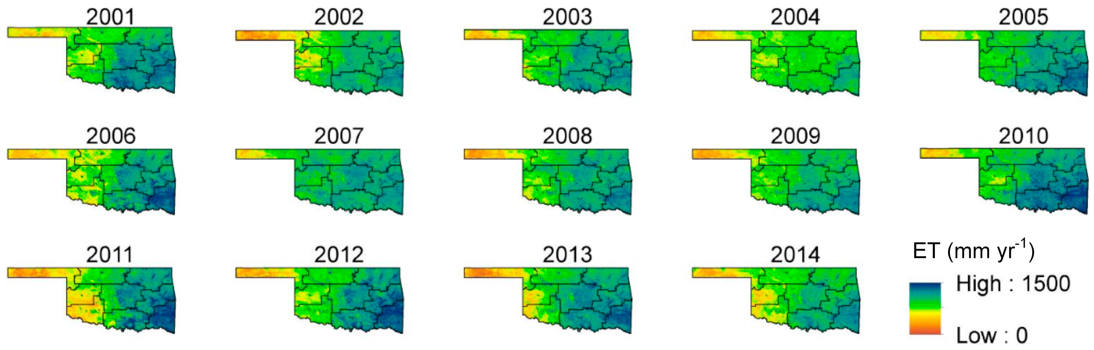
The automated operational ET modeling framework proposed in this study was used to create annual ET maps covering the entire state of Oklahoma for the period from 2001 to 2014. As expected, the annual ET followed the precipitation pattern and increased from southeast to Panhandle (Figure 4). When averaged over the entire 14 years, the southeast climate division (CD9) had the largest annual ET of 1272 mm yr−1 and the Panhandle climate division (CD1) had the smallest annual ET of 588 mm yr−1 (Table 2). The reference ET (ETr) had an opposite pattern, with CD1 having the largest amount at 2140 mm yr−1 and CD9 the smallest (1360 mm yr−1). This means that on average, about 94% of atmospheric demand was fulfilled at southeast, compared to only 27% in the Panhandle during the study period. In other words, water scarcity is a larger issue in CD1 compared to CD9 as available resources were not sufficient to keep up with atmospheric demand. The statewide average annual ET was 994 mm yr−1, about 57% of the average annual ETr of 1755 mm yr−1.
The average annual ET comparison between MOD16 and SEBS indicated large differences across all Oklahoma CDs (Table 2). The differences between MOD16-ET and SEBS-ET varied between 37% at CD9 to 60% at CD2, with an average of 48% lower ET rates from MOD16. Three eastern humid CDs (CD3, CD6, CD9) had smaller differences between MOD16-ET and SEBS-ET compared to three western CDs (CD1, CD4, CD7). The difference between SEBS-ET and MOD16-ET is possibly due to a combination of overestimations from SEBS and underestimation from MOD16. The underestimation of ET from MOD16 has been reported in previous studies, particularly in semi-arid and arid climates [114,115].
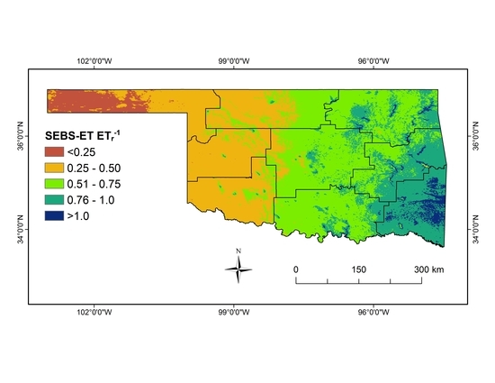
The ratio of SEBS-ET to ETr can be estimated on a pixel wise basis to provide information on water scarcity at a finer resolution for local water management and planning. This ratio is mapped in Figure 5. The general patterns are similar to those presented in Table 2, with western parts of the state under relatively larger water scarcity compared to the eastern parts. However, significant variability can be observed within some CDs. In CD1, for example, the western half of CD (Cimarron and Texas counties) had smaller ratios compared to the eastern half, suggesting a more severe water scarcity. CD2 was similar in terms of variations in the ET ratios across the CD. The surface water resources in western Oklahoma were visible in regions with a ratio value of more than 0.5. Examples include the riparian areas of Cimarron and North Canadian rivers in southwest of CD2, as well as Canton Lake and Foss reservoir in CD4 and the five reservoirs in CD7 (Lugert-Altus, Tom Steed, Lawtonka, Ellsworth and Fort Cobb). Maps similar to the one in Figure 5 can be developed at varying temporal and spatial scales to monitor changes in water availability more closely. The ratio of actual ET to reference or potential ET has been used in the past in monitoring water stress and drought, such as in the Evaporative Stress Index [17].
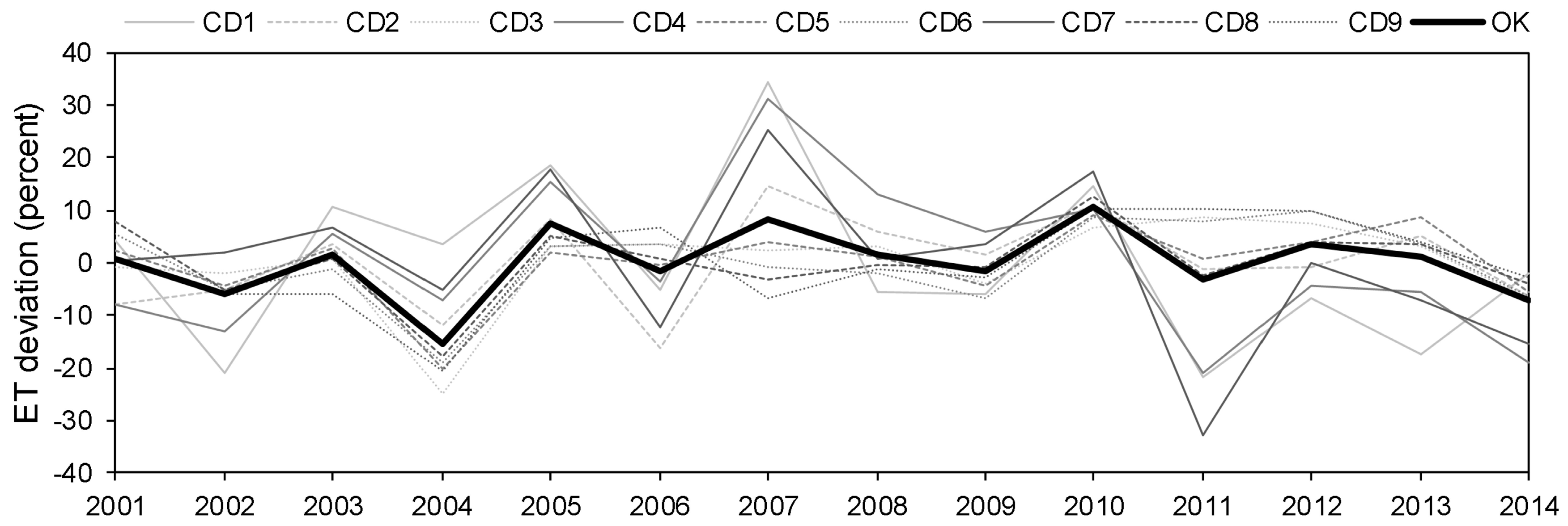
The inter-annual variations in ET were also examined for each CD and for the entire state. Figure 6 demonstrates deviations in SEBS-ET as percentage of the average annual ET during the 2001–2014 period. The impact of the 2011–2014 drought in western Oklahoma can be observed in this graph, with the maximum reduction in ET occurring in 2011 for the three western CDs of CD1, CD4 and CD7. The percent deviations from average was −22%, −21% and −33% for the same CDs, respectively. According to the U.S. Drought Monitor (USDM) [116], more than 80% of the three CDs was under extreme drought (D3 category) from June. The drought condition worsened in July and remained under D4 category until December 2011. The three eastern CDs of CD3, CD6 and CD9 were above average in 2011, with percent deviations of 9%, 8% and 10%, respectively. The USDM indicated almost no drought at CD3 in 2011, whereas CD6 and CD9 had less than 40% of their area under extreme drought from August to November 2011. The middle three CDs registered close to long-term average ET. The largest positive deviations for the three western CDs occurred in 2007, a year that was characterized by above normal precipitation.
The ET modeling framework proposed in this study can automatically generate time series of daily ET maps on a continuous basis, with several applications beyond those mentioned in previous sections. For example, ET maps over agricultural areas can be analyzed in conjunction with yield data to evaluate the water use efficiency. However, this modeling framework has some limitations that must be considered and improved in future applications. One limitation is the size of MODIS pixels, which practically hinders the possibility of using the ET data at field scale. This limitation can be overcome by modifying the framework to use satellite imagery at finer resolution (e.g., Landsat). Another challenge is identifying and removing cloud contaminated pixels. The filters used in this study were not always effective in identifying pixels that were covered by thin layers of cloud or were in the shadow of a cloud. Thus, further investigation and application of robust methods to examine cloud contamination are needed. Finally, there were periods when no images were available for several days due to clouds covering the entire scene. This negatively affects the ability to capture ET fluctuations during those periods. Data-fusion approaches can be implemented in the modeling framework as a potential solution to improving ET interpolation for days with missing images.
4. Conclusions
An ET modeling framework was proposed to automatically construct daily time series of ET maps across Oklahoma by integrating MODIS imagery, ground-based weather data and surface energy balance model. The comparison of the results with daily observations at three flux towers (two years of data at each site) showed good performance of the modeling framework with mean bias errors less than 30 W m−2 and root mean squared errors less than 50 W m−2. The results were then used to investigate spatial and temporal variations in ET across the state and its nine climate divisions (CD). The statewide annual ET varied between 841 and 1100 mm yr−1 during the period from 2001 to 2014, with an average of 994 mm yr−1. A large difference in ET was observed among CDs, with Oklahoma Panhandle (CD1) having the smallest and southeast (CD9) the largest average annual ET of 588 and 1272 mm yr−1, respectively. The ratio of estimated ET to reference ET was used as an indicator of water scarcity at pixel and CD levels. The deviations in annual ET from the 2001–2014 average ET were also studied and found to be in good agreement with temporal and spatial variations in drought. The proposed ET modeling framework provided a pathway to construct daily time series of ET maps with potential for a range of applications. However, further improvements are necessary to resolve the issues highlighted in the current study.
Author Contributions
Conceptualization, P.G. and G.P.; methodology, P.G. and G.P.; formal analysis, K.K., P.G. and G.P.; investigation, K.K., S.T. and P.G.; writing—original draft preparation, K.K. and S.T.; writing—review and editing, K.K., S.T. and P.G.; project administration, S.T. and P.G.; funding acquisition, S.T. and P.G.
Funding
This research was funded by a joint research and extension program funded by the Oklahoma Agricultural Experiment Station (Hatch funds) and Oklahoma Cooperative Extension (Smith-Lever funds) received from the National Institutes for Food and Agriculture, U.S. Department of Agriculture. Additional support was provided by the Oklahoma Water Resources Center through the U.S. Geological Survey 104(b) grants program.
Conflicts of Interest
The authors declare no conflict of interest.
References
- Allen, R.G.; Tasumi, M.; Morse, A.; Trezza, R. A Landsat-based energy balance and evapotranspiration model in Western US water rights regulation and planning. Irrig. Drain. Syst. 2005, 19, 251–268. [Google Scholar] [CrossRef]
- Droogers, P.; Bastiaanssen, W. Irrigation performance using hydrological and remote sensing modeling. J. Irrig. Drain. Eng. 2002, 128, 11–18. [Google Scholar] [CrossRef]
- Santos, C.; Lorite, I.J.; Tasumi, M.; Allen, R.G.; Fereres, E. Performance assessment of an irrigation scheme using indicators determined with remote sensing techniques. Irrig. Sci. 2010, 28, 461–477. [Google Scholar] [CrossRef] [Green Version]
- Taghvaeian, S.; Neale, C.M.; Osterberg, J.C.; Sritharan, S.I.; Watts, D.R. Remote Sensing and GIS Techniques for Assessing Irrigation Performance: Case Study in Southern California. J. Irrig. Drain. Eng. 2018, 144, 05018002. [Google Scholar] [CrossRef]
- Taghvaeian, S.; Neale, C.M. Water balance of irrigated areas: A remote sensing approach. Hydrol. Process. 2011, 25, 4132–4141. [Google Scholar] [CrossRef]
- Folhes, M.T.; Rennó, C.D.; Soares, J.V. Remote sensing for irrigation water management in the semi-arid Northeast of Brazil. Agric. Water Manag. 2009, 96, 1398–1408. [Google Scholar] [CrossRef]
- Bastiaanssen, W.G.M.; Noordman, E.J.M.; Pelgrum, H.; Davids, G.; Thoreson, B.P.; Allen, R.G. SEBAL model with remotely sensed data to improve water-resources management under actual field conditions. J. Irrig. Drain. Eng. 2005, 131, 85–93. [Google Scholar] [CrossRef]
- Anderson, M.C.; Allen, R.G.; Morse, A.; Kustas, W.P. Use of Landsat thermal imagery in monitoring evapotranspiration and managing water resources. Remote Sens. Environ. 2012, 122, 50–65. [Google Scholar] [CrossRef]
- Yao, Y.; Liang, S.; Qin, Q.; Wang, K. Monitoring drought over the conterminous United States using MODIS and NCEP Reanalysis-2 data. J. Appl. Meteorol. Climatol. 2010, 49, 1665–1680. [Google Scholar] [CrossRef]
- Anderson, M.C.; Hain, C.; Wardlow, B.; Pimstein, A.; Mecikalski, J.R.; Kustas, W.P. Evaluation of drought indices based on thermal remote sensing of evapotranspiration over the continental United States. J. Clim. 2011, 24, 2025–2044. [Google Scholar] [CrossRef]
- Zhang, J.; Mu, Q.; Huang, J. Assessing the remotely sensed Drought Severity Index for agricultural drought monitoring and impact analysis in North China. Ecol. Indic. 2016, 63, 296–309. [Google Scholar] [CrossRef]
- Moorhead, J.E.; Gowda, P.H.; Singh, V.P.; Porter, D.O.; Marek, T.H.; Howell, T.A.; Stewart, B.A. Identifying and evaluating a suitable index for agricultural drought monitoring in the Texas high plains. J. Am. Water Resour. Assoc. 2015, 51, 807–820. [Google Scholar] [CrossRef]
- Li, H.; Zheng, L.; Lei, Y.; Li, C.; Liu, Z.; Zhang, S. Estimation of water consumption and crop water productivity of winter wheat in North China Plain using remote sensing technology. Agric. Water Manag. 2008, 95, 1271–1278. [Google Scholar] [CrossRef]
- Ahmad, M.U.D.; Turral, H.; Nazeer, A. Diagnosing irrigation performance and water productivity through satellite remote sensing and secondary data in a large irrigation system of Pakistan. Agric. Water Manag. 2009, 96, 551–564. [Google Scholar] [CrossRef]
- Teixeira, A.D.C.; Bastiaanssen, W.G.M.; Ahmad, M.U.D.; Bos, M.G. Reviewing SEBAL input parameters for assessing evapotranspiration and water productivity for the Low-Middle Sao Francisco River basin, Brazil: Part A: Calibration and validation. Agric. For. Meteorol. 2009, 149, 462–476. [Google Scholar] [CrossRef]
- Cai, X.L.; Sharma, B.R. Integrating remote sensing, census and weather data for an assessment of rice yield, water consumption and water productivity in the Indo-Gangetic river basin. Agric. Water Manag. 2010, 97, 309–316. [Google Scholar] [CrossRef]
- Anderson, M.C.; Zolin, C.A.; Sentelhas, P.C.; Hain, C.R.; Semmens, K.; Yilmaz, M.T.; Gao, F.; Otkin, J.A.; Tetrault, R. The Evaporative Stress Index as an indicator of agricultural drought in Brazil: An assessment based on crop yield impacts. Remote Sens. Environ. 2016, 174, 82–99. [Google Scholar] [CrossRef] [Green Version]
- Oberg, J.W.; Melesss, A.M. Evapotranspiration dynamics at an ecohydrological restoration site: An energy balance and remote sensing approach. J. Am. Water Resour. Assoc. 2006, 42, 565–582. [Google Scholar] [CrossRef]
- Nepstad, D.; Lefebvre, P.; Lopes da Silva, U.; Tomasella, J.; Schlesinger, P.; Solorzano, L.; Moutinho, P.; Ray, D.; Guerreira Benito, J. Amazon drought and its implications for forest flammability and tree growth: A basin-wide analysis. Glob. Chang. Biol. 2004, 10, 704–717. [Google Scholar] [CrossRef]
- Bawazir, A.S.; Samani, Z.; Bleiweiss, M.; Skaggs, R.; Schmugge, T. Using ASTER satellite data to calculate riparian evapotranspiration in the Middle Rio Grande, New Mexico. Int. J. Remote Sens. 2009, 30, 5593–5603. [Google Scholar] [CrossRef]
- Taghvaeian, S.; Neale, C.M.; Osterberg, J.; Sritharan, S.I.; Watts, D.R. Water use and stream-aquifer-phreatophyte interaction along a Tamarisk-dominated segment of the Lower Colorado River. In Remote Sensing of the Terrestrial Water Cycle; John & Sons, Inc.: Hoboken, NJ, USA, 2014; pp. 95–113. [Google Scholar]
- Nagler, P.L.; Glenn, E.P.; Nguyen, U.; Scott, R.L.; Doody, T. Estimating riparian and agricultural actual evapotranspiration by reference evapotranspiration and MODIS enhanced vegetation index. Remote Sens. 2013, 5, 3849–3871. [Google Scholar] [CrossRef]
- Khand, K.; Taghvaeian, S.; Hassan-Esfahani, L. Mapping Annual Riparian Water Use Based on the Single-Satellite-Scene Approach. Remote Sens. 2017, 9, 832. [Google Scholar] [CrossRef]
- Chen, J.M.; Chen, X.; Ju, W.; Geng, X. Distributed hydrological model for mapping evapotranspiration using remote sensing inputs. J. Hydrol. 2005, 305, 15–39. [Google Scholar] [CrossRef]
- Immerzeel, W.W.; Gaur, A.; Zwart, S.J. Integrating remote sensing and a process-based hydrological model to evaluate water use and productivity in a south Indian catchment. Agric. Water Manag. 2008, 95, 11–24. [Google Scholar] [CrossRef]
- Herman, M.R.; Nejadhashemi, A.P.; Abouali, M.; Hernandez-Suarez, J.S.; Daneshvar, F.; Zhang, Z.; Anderson, M.C.; Sadeghi, A.M.; Hain, C.R.; Sharifi, A. Evaluating the role of evapotranspiration remote sensing data in improving hydrological modeling predictability. J. Hydrol. 2018, 556, 39–49. [Google Scholar] [CrossRef]
- Vinukollu, R.K.; Wood, E.F.; Ferguson, C.R.; Fisher, J.B. Global estimates of evapotranspiration for climate studies using multi-sensor remote sensing data: Evaluation of three process-based approaches. Remote Sens. Environ. 2011, 115, 801–823. [Google Scholar] [CrossRef]
- Gowda, P.H.; Chavez, J.L.; Colaizzi, P.D.; Evett, S.R.; Howell, T.A.; Tolk, J.A. Remote sensing based energy balance algorithms for mapping ET: Current status and future challenges. Trans. ASABE 2007, 50, 1639–1644. [Google Scholar] [CrossRef]
- Kalma, J.D.; McVicar, T.R.; McCabe, M.F. Estimating land surface evaporation: A review of methods using remotely sensed surface temperature data. Surv. Geophys. 2008, 29, 421–469. [Google Scholar] [CrossRef]
- Li, Z.L.; Tang, R.; Wan, Z.; Bi, Y.; Zhou, C.; Tang, B.; Yan, G.; Zhang, X. A review of current methodologies for regional evapotranspiration estimation from remotely sensed data. Sensors 2009, 9, 3801–3853. [Google Scholar] [CrossRef] [PubMed]
- Liou, Y.A.; Kar, S.K. Evapotranspiration estimation with remote sensing and various surface energy balance algorithms—A review. Energies 2014, 7, 2821–2849. [Google Scholar] [CrossRef]
- Menenti, M.; Choudhury, B. Parameterization of land surface evaporation by means of location dependent potential evaporation and surface temperature range. Proc. IAHS Conf. Land Surf. Process. 1993, 212, 561–568. [Google Scholar]
- Norman, J.M.; Becker, F. Terminology in thermal infrared remote sensing of natural surfaces. Agric. For. Meteorol. 1995, 77, 153–166. [Google Scholar] [CrossRef]
- Kustas, W.P.; Norman, J.M. Evaluation of soil and vegetation heat flux predictions using a simple two-source model with radiometric temperatures for partial canopy cover. Agric. For. Meteorol. 1999, 94, 13–29. [Google Scholar] [CrossRef]
- Bastiaanssen, W.G.M.; Menenti, M.; Feddes, R.A.; Holtslag, A.A.M. A remote sensing surface energy balance algorithm for land (SEBAL): 1. Formulation. J. Hydrol. 1998, 212, 198–212. [Google Scholar] [CrossRef]
- Roerink, G.; Su, Z.; Menenti, M. S-SEBI: A simple remote sensing algorithm to estimate the surface energy balance. Phys. Chem. Earth Part B Hydrol. Oceans Atmos. 2000, 25, 147–157. [Google Scholar] [CrossRef]
- Su, Z. The surface energy balance system (SEBS) for estimation of turbulent heat fluxes. Hydrol. Earth Syst. Sci. 2002, 6, 85–99. [Google Scholar] [CrossRef]
- Allen, R.G.; Tasumi, M.; Trezza, R. Satellite-based energy balance for mapping evapotranspiration with internalized calibration (METRIC)-model. J. Irrig. Drain. Eng. 2007, 133, 380–394. [Google Scholar] [CrossRef]
- Anderson, M.C.; Norman, J.M.; Mecikalski, J.R.; Otkin, J.A.; Kustas, W.P. A climatological study of evapotranspiration and moisture stress across the continental United States based on thermal remote sensing: 1. Model formulation. J. Geophys. Res. Atmos. 2007, 112, D11112. [Google Scholar] [CrossRef]
- Samani, Z.; Bawazir, A.S.; Skaggs, R.K.; Bleiweiss, M.P.; Piñon, A.; Tran, V. Water use by agricultural crops and riparian vegetation: An application of remote sensing technology. J. Contemp. Water Res. Educ. 2007, 137, 8–13. [Google Scholar] [CrossRef]
- Elhaddad, A.; Garcia, L.A. Surface energy balance-based model for estimating evapotranspiration taking into account spatial variability in weather. J. Irrig. Drain. Eng. 2008, 134, 681–689. [Google Scholar] [CrossRef]
- Senay, G.B.; Bohms, S.; Singh, R.K.; Gowda, P.H.; Velpuri, N.M.; Alemu, H.; Verdin, J.P. Operational evapotranspiration mapping using remote sensing and weather datasets: A new parameterization for the SSEB approach. J. Am. Water Resour. Assoc. 2013, 49, 577–591. [Google Scholar] [CrossRef]
- Yang, Y.; Long, D.; Shang, S. Remote estimation of terrestrial evapotranspiration without using meteorological data. Geophys. Res. Lett. 2013, 40, 3026–3030. [Google Scholar] [CrossRef] [Green Version]
- Timmermans, W.J.; Kustas, W.P.; Anderson, M.C.; French, A.N. An intercomparison of the surface energy balance algorithm for land (SEBAL) and the two-source energy balance (TSEB) modeling schemes. Remote Sens. Environ. 2007, 108, 369–384. [Google Scholar] [CrossRef]
- Allen, R.G.; Pereira, L.S.; Howell, T.A.; Jensen, M.E. Evapotranspiration information reporting: I. Factors governing measurement accuracy. Agric. Water Manag. 2011, 98, 899–920. [Google Scholar] [CrossRef]
- Fisher, J.B.; Whittaker, R.J.; Malhi, Y. ET come home: Potential evapotranspiration in geographical ecology. Glob. Ecol. Biogeogr. 2011, 20, 1–18. [Google Scholar] [CrossRef]
- Allen, R.G. Assessing integrity of weather data for reference evapotranspiration estimation. J. Irrig. Drain. Eng. 1996, 122, 97–106. [Google Scholar] [CrossRef]
- Environmental and Water Resources Institute for the American Society of Civil Engineers (ASCE-EWRI). The ASCE Standardized Reference Evapotranspiration Equation; Report of the ASCE-EWRI Task Committee on Standardization of Reference Evapotranspiration; ASCE: Reston, VA, USA, 2005.
- Webster, E.; Ramp, D.; Kingsford, R.T. Spatial sensitivity of surface energy balance algorithms to meteorological data in a heterogeneous environment. Remote Sens. Environ. 2016, 187, 294–319. [Google Scholar] [CrossRef]
- Senay, G.B.; Friedrichs, M.; Singh, R.K.; Velpuri, N.M. Evaluating Landsat 8 evapotranspiration for water use mapping in the Colorado River Basin. Remote Sens. Environ. 2016, 185, 171–185. [Google Scholar] [CrossRef] [Green Version]
- Biggs, T.W.; Marshall, M.; Messina, A. Mapping daily and seasonal evapotranspiration from irrigated crops using global climate grids and satellite imagery: Automation and methods comparison. Water Resour. Res. 2016, 52, 7311–7326. [Google Scholar] [CrossRef]
- Moorhead, J.; Gowda, P.; Hobbins, M.; Senay, G.; Paul, G.; Marek, T.; Porter, D. Accuracy assessment of NOAA gridded daily reference evapotranspiration for the Texas High Plains. J. Am. Water Resour. Assoc. 2015, 51, 1262–1271. [Google Scholar] [CrossRef]
- Porter, D.; Gowda, P.; Marek, T.; Howell, T.; Moorhead, J.; Irmak, S. Sensitivity of grass-and alfalfa-reference evapotranspiration to weather station sensor accuracy. Appl. Eng. Agric. 2012, 28, 543–549. [Google Scholar] [CrossRef]
- Elhaddad, A.; Garcia, L.A. ReSET-Raster: Surface energy balance model for calculating evapotranspiration using a raster approach. J. Irrig. Drain. Eng. 2011, 137, 203–210. [Google Scholar] [CrossRef]
- Kustas, W.P.; Humes, K.S.; Norman, J.M.; Moran, M.S. Single-and dual-source modeling of surface energy fluxes with radiometric surface temperature. J. Appl. Meteorol. 1996, 35, 110–121. [Google Scholar] [CrossRef]
- Long, D.; Singh, V.P. A modified surface energy balance algorithm for land (M-SEBAL) based on a trapezoidal framework. Water Resour. Res. 2012, 48, W02528. [Google Scholar] [CrossRef]
- Kjaersgaard, J.H.; Allen, R.G.; Garcia, M.; Kramber, W.; Trezza, R. Automated selection of anchor pixels for Landsat based evapotranspiration estimation. In Proceedings of the World Environmental and Water Resources Congress, Kansas City, MO, USA, 17–21 May 2009. [Google Scholar]
- Allen, R.G.; Burnett, B.; Kramber, W.; Huntington, J.; Kjaersgaard, J.; Kilic, A.; Kelly, C.; Trezza, R. Automated calibration of the METRIC-Landsat evapotranspiration process. J. Am. Water Resour. Assoc. 2013, 49, 563–576. [Google Scholar] [CrossRef]
- Bhattarai, N.; Quackenbush, L.J.; Im, J.; Shaw, S.B. A new optimized algorithm for automating endmember pixel selection in the SEBAL and METRIC models. Remote Sens. Environ. 2017, 196, 178–192. [Google Scholar] [CrossRef]
- Trezza, R.; Allen, R.G.; Tasumi, M. Estimation of actual evapotranspiration along the Middle Rio Grande of New Mexico using MODIS and Landsat imagery with the METRIC model. Remote Sens. 2013, 5, 5397–5423. [Google Scholar] [CrossRef]
- Khand, K.; Numata, I.; Kjaersgaard, J.; Vourlitis, G.L. Dry Season Evapotranspiration Dynamics over Human-Impacted Landscapes in the Southern Amazon Using the Landsat-Based METRIC Model. Remote Sens. 2017, 9, 706. [Google Scholar] [CrossRef]
- Brutsaert, W.; Sugita, M. Application of self-preservation in the diurnal evolution of the surface energy budget to determine daily evaporation. J. Geophys. Res. Atmos. 1992, 97, 18377–18382. [Google Scholar] [CrossRef]
- Kustas, W.P.; Perry, E.M.; Doraiswamy, P.C.; Moran, M.S. Using satellite remote sensing to extrapolate evapotranspiration estimates in time and space over a semiarid rangeland basin. Remote Sens. Environ. 1994, 49, 275–286. [Google Scholar] [CrossRef]
- Trezza, R. Evapotranspiration Using a Satellite-Based Surface Energy Balance with Standardized Ground Control. Ph.D. Thesis, Biological and Irrigation Engineering Department, Utah State University, Logan, UT, USA, 2002. [Google Scholar]
- Gentine, P.; Entekhabi, D.; Chehbouni, A.; Boulet, G.; Duchemin, B. Analysis of evaporative fraction diurnal behaviour. Agric. For. Meteorol. 2007, 143, 13–29. [Google Scholar] [CrossRef] [Green Version]
- Colaizzi, P.D.; Evett, S.R.; Howell, T.A.; Tolk, J.A. Comparison of five models to scale daily evapotranspiration from one-time-of-day measurements. Trans. ASABE 2006, 49, 1409–1417. [Google Scholar] [CrossRef]
- Chávez, J.L.; Neale, C.M.; Prueger, J.H.; Kustas, W.P. Daily evapotranspiration estimates from extrapolating instantaneous airborne remote sensing ET values. Irrig. Sci. 2008, 27, 67–81. [Google Scholar] [CrossRef]
- Delogu, E.; Boulet, G.; Olioso, A.; Coudert, B.; Chirouze, J.; Ceschia, E.; Le Dantec, V.; Marloie, O.; Chehbouni, G.; Lagouarde, J.P. Reconstruction of temporal variations of evapotranspiration using instantaneous estimates at the time of satellite overpass. Hydrol. Earth Syst. Sci. 2012, 16, 2995–3010. [Google Scholar] [CrossRef] [Green Version]
- Kjaersgaard, J.; Allen, R.; Trezza, R.; Robison, C.; Oliveira, A.; Dhungel, R.; Kra, E. Filling satellite image cloud gaps to create complete images of evapotranspiration. In Proceedings of the Remote Sensing and Hydrology 2010 Symposium, Jackson Hole, WY, USA, 27–30 September 2010. [Google Scholar]
- Singh, R.K.; Liu, S.; Tieszen, L.L.; Suyker, A.E.; Verma, S.B. Estimating seasonal evapotranspiration from temporal satellite images. Irrig. Sci. 2012, 30, 303–313. [Google Scholar] [CrossRef]
- Kjaersgaard, J.; Allen, R.; Irmak, A. Improved methods for estimating monthly and growing season ET using METRIC applied to moderate resolution satellite imagery. Hydrol. Process. 2011, 25, 4028–4036. [Google Scholar] [CrossRef]
- Khand, K.; Kjaersgaard, J.; Hay, C.; Jia, X. Estimating impacts of agricultural subsurface drainage on evapotranspiration using the Landsat imagery-based METRIC model. Hydrology 2017, 4, 49. [Google Scholar] [CrossRef]
- Dhungel, R.; Allen, R.G.; Trezza, R.; Robison, C.W. Evapotranspiration between satellite overpasses: Methodology and case study in agricultural dominant semi-arid areas. Meteorol. Appl. 2016, 23, 714–730. [Google Scholar] [CrossRef]
- Kottek, M.; Grieser, J.; Beck, C.; Rudolf, B.; Rubel, F. World map of the Köppen-Geiger climate classification updated. Meteorol. Z. 2006, 15, 259–263. [Google Scholar] [CrossRef]
- Homer, C.; Dewitz, J.; Yang, L.; Jin, S.; Danielson, P.; Xian, G.; Coulston, J.; Herold, N.; Wickham, J.; Megown, K. Completion of the 2011 National Land Cover Database for the conterminous United States–representing a decade of land cover change information. Photogramm. Eng. Remote Sens. 2015, 81, 345–354. [Google Scholar]
- Vermote, E.; Wolfe, R. MOD09GA MODIS/Terra Surface Reflectance Daily L2G Global 1 km and 500 m SIN Grid V006; NASA EOSDIS LP DAAC; NASA: Washington, DC, USA, 2015. [CrossRef]
- Wan, Z.; Hook, S.; Hulley, G. MOD11A1 MODIS/Terra Land Surface Temperature/Emissivity Daily L3 Global 1km SIN Grid V006; NASA EOSDIS LP DAAC; NASA: Washington, DC, USA, 2015. [CrossRef]
- Brock, F.V.; Crawford, K.C.; Elliott, R.L.; Cuperus, G.W.; Stadler, S.J.; Johnson, H.L.; Eilts, M.D. The Oklahoma Mesonet: A technical overview. J. Atmos. Ocean. Technol. 1995, 12, 5–19. [Google Scholar] [CrossRef]
- McPherson, R.A.; Fiebrich, C.A.; Crawford, K.C.; Kilby, J.R.; Grimsley, D.L.; Martinez, J.E.; Basara, J.B.; Illston, B.G.; Morris, A.D.; Kloesel, K.A.; et al. Statewide monitoring of the mesoscale environment: A technical update on the Oklahoma Mesonet. J. Atmos. Ocean. Technol. 2007, 24, 301–321. [Google Scholar] [CrossRef]
- Gowda, P.H.; Ennis, J.; Howell, T.A.; Marek, T.H.; Porter, D.O. The ASCE Standardized Equation-Based Bushland Reference ET Calculator. In Proceedings of the World Environmental and Water Resources Congress, Albuquerque, NM, USA, 20–24 May 2012. [Google Scholar]
- WMO. Hydrology–From Measurement to Hydrological Information. In Guide to Hydrological Practices; WMO: Geneva, Switzerland, 2008; Volume I. [Google Scholar]
- Liang, S. Narrowband to broadband conversions of land surface albedo I: Algorithms. Remote Sens. Environ. 2001, 76, 213–238. [Google Scholar] [CrossRef]
- Brutsaert, W.H. Evaporation into the Atmosphere; D. Reidel: London, UK, 1982. [Google Scholar]
- Liang, S. Quantitative Remote Sensing of Land Surfaces; John Wiley & Sons: Hoboken, NJ, USA, 2005; pp. 1–528. [Google Scholar]
- Brutsaert, W. Aspect of bulk atmospheric boundary layer similarity under free-convective conditions. Rev Geophys. 1999, 37, 439–451. [Google Scholar] [CrossRef]
- Monin, A.S.; Obukhov, A.M.F. Basic laws of turbulent mixing in the surface layer of the atmosphere. Contrib. Geophys. Inst. Acad. Sci. USSR 1954, 24, 163–187. [Google Scholar]
- Beljaars, A.C.M.; Holtslag, A.A.M. Flux parameterization over land surfaces for atmospheric models. J. Appl. Meteorol. 1991, 30, 327–341. [Google Scholar] [CrossRef]
- Gupta, R.K.; Prasad, T.S.; Vijayan, D. Estimation of roughness length and sensible heat flux from WiFS and NOAA AVHRR data. Adv. Space Res. 2002, 29, 33–38. [Google Scholar] [CrossRef]
- Su, Z.; Schmugge, T.; Kustas, W.P.; Massman, W.J. An evaluation of two models for estimation of the roughness height for heat transfer between the land surface and the atmosphere. J. Appl. Meteorol. 2001, 40, 1933–1951. [Google Scholar] [CrossRef]
- Choudhury, B.J.; Monteith, J.L. A four-layer model for the heat budget of homogeneous land surfaces. Q. J. R. Meteorol. Soc. 1988, 114, 373–398. [Google Scholar] [CrossRef]
- Gowda, P.H.; Chavez, J.L.; Colaizzi, P.D.; Howell, T.A.; Schwartz, R.C.; Marek, T.H. Relationship between LAI and Landsat TM spectral vegetation indices in the Texas Panhandle. In Proceedings of the American Society of Agricultural and Biological Engineers Annual Meeting, Minneapolis, MI, USA, 17–20 June 2007. [Google Scholar]
- Monteith, J.L. Evaporation and the Environment: The State and Movement of Water in Living Organism; XIXth Symposium; Cambridge University Press: Swansea, UK, 1965. [Google Scholar]
- Monteith, J.L. Evaporation and surface temperature. Q. J. R. Meteorol. Soc. 1981, 107, 1–27. [Google Scholar] [CrossRef]
- Fischer, M.L.; Torn, M.S.; Billesbach, D.P.; Doyle, G.; Northup, B.; Biraud, S.C. Carbon, water, and heat flux responses to experimental burning and drought in a tallgrass prairie. Agric. For. Meteorol. 2012, 166, 169–174. [Google Scholar] [CrossRef]
- Billesbach, D.; Bradford, J.; Margaret, T. AmeriFlux US-AR2 ARM USDA UNL OSU Woodward Switchgrass 2; U.S. Department of Agriculture: Washington, DC, USA; University of Nebraska: Lincoln, NE, USA, 2015.
- Twine, T.E.; Kustas, W.P.; Norman, J.M.; Cook, D.R.; Houser, P.R.; Meyers, T.P.; Prueger, J.H.; Starks, P.J.; Wesely, M.L. Correcting Eddy-Covariance Flux Underestimates over a Grassland. Agric. For. Meteorol. 2000, 103, 279–300. [Google Scholar] [CrossRef]
- Mu, Q.; Heinsch, F.A.; Zhao, M.; Running, S.W. Development of a global evapotranspiration algorithm based on MODIS and global meteorology data. Remote Sens. Environ. 2007, 111, 519–536. [Google Scholar] [CrossRef]
- Mu, Q.; Zhao, M.; Running, S.W. Improvements to a MODIS global terrestrial evapotranspiration algorithm. Remote Sens. Environ. 2011, 115, 1781–1800. [Google Scholar] [CrossRef]
- Gokmen, M.; Vekerdy, Z.; Verhoef, A.; Verhoef, W.; Batelaan, O.; Van der Tol, C. Integration of soil moisture in SEBS for improving evapotranspiration estimation under water stress conditions. Remote Sens. Environ. 2012, 121, 261–274. [Google Scholar] [CrossRef]
- Gibson, L.A. The Application of the Surface Energy Balance System Model to Estimate Evapotranspiration in South Africa. Ph.D. Thesis, University of Cape Town, Cape Town, South Africa, 2013. [Google Scholar]
- Paul, G.; Gowda, P.H.; Prasad, P.V.; Howell, T.A.; Aiken, R.M.; Neale, C.M. Investigating the influence of roughness length for heat transport (zoh) on the performance of SEBAL in semi-arid irrigated and dryland agricultural systems. J. Hydrol. 2014, 509, 231–244. [Google Scholar] [CrossRef]
- Bhattarai, N.; Mallick, K.; Brunsell, N.A.; Sun, G.; Jain, M. Regional evapotranspiration from image-based implementation of the Surface Temperature Initiated Closure (STIC1. 2) model and its validation across an aridity gradient in the conterminous United States. Hydrol. Earth Syst. Sci. 2018, 22, 2311–2341. [Google Scholar] [CrossRef]
- Khan, I.S.; Hong, Y.; Vieux, B.; Liu, W. Development and evaluation of an actual evapotranspiration estimation algorithm using satellite remote sensing and meteorological observational network in Oklahoma. Int. J. Remote Sens. 2010, 31, 3799–3819. [Google Scholar] [CrossRef]
- Liaqat, U.W.; Choi, M. Accuracy comparison of remotely sensed evapotranspiration products and their associated water stress footprints under different land cover types in Korean peninsula. J. Clean. Prod. 2017, 155, 93–104. [Google Scholar] [CrossRef]
- Yang, Z.; Zhang, Q.; Yang, Y.; Hao, X.; Zhang, H. Evaluation of evapotranspiration models over semi-arid and semi-humid areas of China. Hydrol. Process. 2016, 30, 4292–4313. [Google Scholar] [CrossRef]
- Li, Y.; Huang, C.; Hou, J.; Gu, J.; Zhu, G.; Li, X. Mapping daily evapotranspiration based on spatiotemporal fusion of ASTER and MODIS images over irrigated agricultural areas in the Heihe River Basin, Northwest China. Agric. For. Meteorol. 2017, 244, 82–97. [Google Scholar] [CrossRef]
- Huang, C.; Li, Y.; Gu, J.; Lu, L.; Li, X. Improving estimation of evapotranspiration under water-limited conditions based on SEBS and MODIS data in arid regions. Remote Sens. 2015, 7, 16795–16814. [Google Scholar] [CrossRef]
- Kustas, W.P.; Norman, J.M. Evaluating the effects of subpixel heterogeneity on pixel average fluxes. Remote Sens. Environ. 2000, 74, 327–342. [Google Scholar] [CrossRef]
- Van der Kwast, J.; Timmermans, W.; Gieske, A.; Su, Z.; Olioso, A.; Jia, L.; Elbers, J.; Karssenberg, D.; de Jong, S. Evaluation of the Surface Energy Balance System (SEBS) applied to ASTER imagery with flux-measurements at the SPARC 2004 site (Barrax, Spain). Hydrol. Earth Syst. Sci. Discuss. 2009, 6, 1165–1196. [Google Scholar] [CrossRef]
- Liaqat, U.W.; Choi, M.; Awan, U.K. Spatio-temporal distribution of actual evapotranspiration in the Indus Basin Irrigation System. Hydrol. Process. 2015, 29, 2613–2627. [Google Scholar] [CrossRef]
- Wang, Y.; Li, X.; Tang, S. Validation of the SEBS-derived sensible heat for FY3A/VIRR and TERRA/MODIS over an alpine grass region using LAS measurements. Int. J. Appl. Earth Obs. Geoinf. 2013, 23, 226–233. [Google Scholar] [CrossRef]
- Gibson, L.A.; Münch, Z.; Engelbrecht, J. Particular uncertainties encountered in using a pre-packaged SEBS model to derive evapotranspiration in a heterogeneous study area in South Africa. Hydrol. Earth Syst. Sci. 2011, 15, 295–310. [Google Scholar] [CrossRef] [Green Version]
- Su, H.; Wood, E.F.; McCabe, M.F.; Su, Z. Evaluation of remotely sensed evapotranspiration over the CEOP EOP-1 reference sites. J. Meteorol. Soc. Jpn. 2007, 85, 439–459. [Google Scholar] [CrossRef]
- Hu, G.; Jia, L.; Menenti, M. Comparison of MOD16 and LSA-SAF MSG evapotranspiration products over Europe for 2011. Remote Sens. Environ. 2015, 156, 510–526. [Google Scholar] [CrossRef]
- Feng, X.M.; Sun, G.; Fu, B.J.; Su, C.H.; Liu, Y.; Lamparski, H. Regional effects of vegetation restoration on water yield across the Loess Plateau, China. Hydrol. Earth Syst. Sci. 2012, 16, 2617–2628. [Google Scholar] [CrossRef] [Green Version]
- Svoboda, M.; LeComte, D.; Hayes, M.; Heim, R.; Gleason, K.; Angel, J.; Rippey, B.; Tinker, R.; Palecki, M.; Stooksbury, D.; et al. The drought monitor. Bull. Am. Meteorol. Soc. 2002, 83, 1181–1190. [Google Scholar] [CrossRef]
Figure 1.
Map of Oklahoma and its nine climate divisions. The locations of Mesonet stations and flux towers are also specified.
Figure 1.
Map of Oklahoma and its nine climate divisions. The locations of Mesonet stations and flux towers are also specified.

Figure 2.
A descriptive flow diagram of the daily time series of evapotranspiration (ET) modeling framework.
Figure 2.
A descriptive flow diagram of the daily time series of evapotranspiration (ET) modeling framework.

Figure 3.
Comparison of daily ET from surface energy balances (SEBS) and flux tower (FT).

Figure 4.
Annual ET maps (SEBS-ET) of Oklahoma from 2001 to 2014. The solid lines represent boundaries of the nine climate divisions. It should be noted that CDs 6 and 9 in southeast have a forested area of more than 29%. Hence, their ET estimates may not be accurate since the flux towers used in validation did not include forest land cover.

Figure 5.
The ratio of average annual SEBS-ET to ETr across Oklahoma during the period 2001–2014. It should be noted that CDs 6 and 9 in southeast have a forested area of more than 29%. Hence, their ET estimates may not be accurate since the flux towers used in validation did not include forest land cover.

Figure 6.
Annual ET deviation across climate divisions of Oklahoma from 2001 to 2014.


Table 1.
Statistical indicators between SEBS and flux tower ET.
| Site | Year | r | R2 | MAE (W m−2) | MBE (W m−2) | RMSE (W m−2) |
|---|---|---|---|---|---|---|
| US-ARc | 2005 | 0.78 | 0.61 | 39.6 | 19.1 | 40.1 |
| 2006 | 0.77 | 0.59 | 36.7 | 27.5 | 49.2 | |
| US-ARb | 2005 | 0.81 | 0.66 | 31.9 | 26.6 | 43.3 |
| 2006 | 0.78 | 0.61 | 35.9 | 29.3 | 47.7 | |
| US-AR2 | 2010 | 0.61 | 0.37 | 29.4 | 16.4 | 41.7 |
| 2011 | 0.62 | 0.39 | 24.7 | 1.7 | 34.1 |
Table 2.
Average annual SEBS-ET, MOD16-ET, ETr and the ratio of SEBS-ET to ETr for all Oklahoma climate divisions (CD) during the 2001–2014 period.
Table 2.
Average annual SEBS-ET, MOD16-ET, ETr and the ratio of SEBS-ET to ETr for all Oklahoma climate divisions (CD) during the 2001–2014 period.
| Climate Division | SEBS-ET (mm yr−1) | MOD16-ET (mm yr−1) | ETr (mm yr−1) | SEBS-ET ETr−1 |
|---|---|---|---|---|
| CD1 (Panhandle) | 588 | 259 | 2140 | 0.27 |
| CD2 (North Central) | 918 | 364 | 1871 | 0.49 |
| CD3 (Northeast) | 1098 | 657 | 1521 | 0.72 |
| CD4 (West Central) | 790 | 338 | 2018 | 0.39 |
| CD5 (Central) | 1095 | 531 | 1700 | 0.64 |
| CD6 (East Central) * | 1175 | 736 | 1492 | 0.79 |
| CD7 (Southwest) | 845 | 363 | 2009 | 0.42 |
| CD8 (South Central) | 1163 | 599 | 1683 | 0.69 |
| CD9 (Southeast) * | 1272 | 798 | 1360 | 0.94 |
| Oklahoma | 994 | 516 | 1755 | 0.57 |
* These CDs have a forested area of more than 29%. The results presented in this table may not be accurate for these CDs since the flux towers used in validation did not include forest land cover.
© 2019 by the authors. Licensee MDPI, Basel, Switzerland. This article is an open access article distributed under the terms and conditions of the Creative Commons Attribution (CC BY) license (http://creativecommons.org/licenses/by/4.0/).
Share and Cite
MDPI and ACS Style
Khand, K.; Taghvaeian, S.; Gowda, P.; Paul, G. A Modeling Framework for Deriving Daily Time Series of Evapotranspiration Maps Using a Surface Energy Balance Model. Remote Sens. 2019, 11, 508. https://doi.org/10.3390/rs11050508
AMA Style
Khand K, Taghvaeian S, Gowda P, Paul G. A Modeling Framework for Deriving Daily Time Series of Evapotranspiration Maps Using a Surface Energy Balance Model. Remote Sensing. 2019; 11(5):508. https://doi.org/10.3390/rs11050508
Chicago/Turabian StyleKhand, Kul, Saleh Taghvaeian, Prasanna Gowda, and George Paul. 2019. "A Modeling Framework for Deriving Daily Time Series of Evapotranspiration Maps Using a Surface Energy Balance Model" Remote Sensing 11, no. 5: 508. https://doi.org/10.3390/rs11050508
Note that from the first issue of 2016, this journal uses article numbers instead of page numbers. See further details here.