Article

Spatio-Temporal Variations of Carbon Use Efficiency in Natural Terrestrial Ecosystems and the Relationship with Climatic Factors in the Songnen Plain, China

Key Laboratory of Geographical Processes and Ecological Security in Changbai Mountains, Ministry of Education, School of Geographical Sciences, Northeast Normal University, Renmin Street No.5268, Changchun 130024, China
*
Author to whom correspondence should be addressed.
Remote Sens. 2019, 11(21), 2513; https://doi.org/10.3390/rs11212513
Submission received: 30 September 2019 / Revised: 24 October 2019 / Accepted: 25 October 2019 / Published: 27 October 2019
(This article belongs to the Special Issue Remote Sensing Applications in Monitoring of Protected Areas)

Abstract

:
The Songnen Plain (SNP) is an important grain production base, and is designated as an ecological red-line as a protected area in China. Natural ecosystems such as the ecological protection barrier play an important role in maintaining the productivity and sustainability of farmland. Carbon use efficiency (CUE), defined as the ratio of net primary productivity (NPP) to gross primary productivity (GPP), represents the ecosystem capacity of transferring carbon from the atmosphere to terrestrial biomass. The understanding of the CUE of natural ecosystems in protected farmland areas is vital to predicting the impact of global change and human disturbances on carbon budgets and evaluating ecosystem functions. To date, the changes in CUE at different time scales and their relationships with climatic factors have yet to be fully understood. CUE and the response to land surface phenology are also deserving attention. In this study, variations in ecosystem CUE in the SNP during 2001–2015 were investigated using Moderate-Resolution Imaging Spectroradiometer (MODIS) GPP and NPP data products estimated using the Carnegie-Ames-Stanford approach (CASA) model. The relationships between CUE and phenological and climate factors were explored. The results showed that ecosystem CUE fluctuated over time in the SNP. The lowest and highest CUE values mainly occurred in May and October, respectively. At seasonal scale, average CUE followed a descending order of Autumn > Summer > Spring. The CUE of mixed forest was greater than that of other ecosystems at both monthly and seasonal scales. Land surface phenology plays an important role in the regulation of CUE. The earlier start (SOS), the later end (EOS) and longer length (LOS) of the growing season would contribute increasing of CUE. Precipitation and temperature affected CUE positively in most areas of the SNP. These findings help explain the CUE of natural ecosystems in the protected farmland areas and improve our understanding of ecosystem carbon allocation dynamics in temperate semi-humid to semi-arid transitional region under climate and phenological fluctuations.

Graphical Abstract

1. Introduction

In recent decades, driven by intensive human activity and climate change, the function of terrestrial ecosystem has been disturbed and continuously degraded on regional and global scales. The increasing levels of atmospheric CO2 concentrations and climate change have highlighted the need for a better understanding of terrestrial carbon cycling and its responses to climate change. Gross primary production (GPP) represents the capacity of the plants in an ecosystem to capture energy and carbon [1]. Net Primary Productivity (NPP) is defined as the amount of atmospheric carbon that is captured by plants and transformed into biomass [2]. The GPP is the sum of NPP and autotrophic respiration (Ra), and Ra plus heterotrophic respiration (Rh) comprises ecosystem respiration. GPP, NPP and Ra are the most important and highly related constituents of carbon cycling. The carbon fixed by photosynthesis is allocated to a variety of usages in plants, including growth and maintenance respirations and biomass accumulation [3]. About 50–70% of the carbon fixation is returned to the environment through Ra [4,5]. Carbon allocation among plant processes (e.g., respiration, biomass production) and organs (e.g., leaves, stem) is a key process in the carbon cycle because it determines the residence time and location of carbon in the ecosystem [6,7]. For example, the residence times of the carbon used for maintenance respiration and the carbon allocated to the structural biomass of organs are drastically different, ranging from a few hours to a few years [6]. Therefore, the allocation process of carbon is highly relevant to understanding ecosystem carbon stock and carbon cycles [6].
Carbon use efficiency (CUE) is defined as the ratio of NPP to GPP, which indicates the ecosystem capacity in transferring CO2 into biomass and carbon sequestration [8]. CUE is an important functional parameter of ecosystems and can be used for comparing carbon cycle differences in various ecosystems [9]. The index is intuitive and easy to compare between different vegetation types, and to apply to different time scales [7]. A higher CUE indicates a higher growth transfer per unit of carbon sequestration. In practice, GPP usually represents the total amount of carbon captured through photosynthesis, and NPP is the net carbon stored in plant after the reduction of GPP through by plant respiration [1]. CUE is also a measure of how GPP is partitioned into NPP and Ra [7]. Less Ra may result in larger carbon reserve accumulation. Hence, CUE is related to photosynthetic process, and it is also regarded as an important indicator for characterizing ecosystem functions. How efficiently an ecosystem is able to convert GPP into plant and soil storage greatly determines the carbon sequestration of terrestrial ecosystems, so CUE changes strongly affect ecosystem carbon budgets [10]. Quantitative analysis of spatial-temporal changes of CUE and its influencing factors will help better understand the effects of climate change on carbon processes of ecosystems [11].
Satellite remote sensing provides critical information for investigating large-scale and long-term variability of ecosystem CUE. Piao et al. [12] demonstrated that CUE of different vegetation differed greatly from the south temperate to the tropic ecoregions based on a global forest C-flux database, and found that the spatial patterns of forest annual Ra at the global scale were largely controlled by temperature. Zhang et al. [1] reported that CUE exhibited a pattern depending on the climatic characteristics-based upon Moderate-Resolution Imaging Spectroradiometer (MODIS)-derived NPP and GPP data. He et al. [13] investigated spatial variations in CUE from different models and analyzed the responses of CUE to precipitation and temperature. Tang et al. [3] established a global database of site-year CUE based on field observations for five ecosystem types and diagnosed the spatial variability of CUE with climate and other environmental factors (e.g., soil variables). Two prominent gradients of CUE in ecosystem types and latitude were found worldwide. CUE varied with ecosystem types, being the highest in wetland and lowest in grassland. CUE decreased with latitude, showing the lowest values in tropics, and the highest CUE were found in higher-latitude regions. The above studies were based on annual scales and advanced the knowledge of understanding the global pattern of CUE. However, monthly scale analysis of CUE has rarely been studied.
From individual plants to an entire ecosystem, phenology directly or indirectly regulates carbon fluxes (e.g., photosynthesis and respiration) between the land surface and the atmosphere [14] through altering physiological and structural characteristics, including photosynthetic rate, canopy conductance and albedo [14,15,16]. Vegetation phenological changes are closely related to spatial-temporal dynamics of carbon cycle [17]. The change in the length of the growing season may have an important impact on vegetation growth, which will cause changes in the GPP and NPP [18]. CUE and its relationships with land surface phenology (LSP) deserve attention.
The Songnen Plain (SNP), located in temperate semi-humid to semi-arid transition ecological fragile zone in Northeast China, is highly sensitive to global change. As a key agricultural area and important grain commodity base, the SNP is among the designated ecological red-lines as protected farmland area in China. The natural terrestrial ecosystem acts as an ecological protection barrier for the croplands in the SNP. The productivity and sustainability of terrestrial ecosystems are vital to maintaining regional and national food and ecological security. Due to the combined effects of vulnerable physical conditions and excessive human activities, the SNP suffered from high risk of land degradation during the past century. Concerns for the aggravation of desertification have led to many measures and management actions for ecological and environmental protection. The trend of desertification and exacerbation has gradually slowed down [19]. Previous studies have mostly focused on the land cover/use change and effects of agricultural activities on environment [20]. In addition, most studies only focused on the condition of protected farmland, while ignoring the productivity and sustainability of natural terrestrial ecosystems around it. There is a lack of reports about the spatial-temporal patterns of ecosystem-level CUE and their response to phenology and climate change in the SNP region. This study attempts to fill in the gaps in the knowledge regarding biotic and abiotic impacts on CUE of the SNP region.
The objectives of this study are to: (1) estimate CUE of different ecosystems and investigate their monthly and seasonal changes based on MODIS GPP and NPP data from 2001 to 2015; (2) explain how phenology and climatic factors contribute to variations in ecosystem CUE, in order to improve our understanding of the carbon budget in temperate semi-arid and semi-humid transitional zone ecosystems and their driving mechanisms.

2. Materials and Methods

2.1. Study Area

The SNP is located in the central part of Northeast China, in a range of 121°38′ to 128°33′E, 42°49′ to 49°12′N, with a total area of 22.35 × 10⁴ km2 (Figure 1). It is an alluvial plain situated in the central Songliao Basin between the Xiaoxing’an and Changbai Mountains, through which the Songhua River and the Nenjiang River flow [10]. The SNP belongs to a temperate continental semi-humid and semi-arid monsoon climate zone, characterized by four seasons with a hot, rainy summer and a cold, dry winter and with significant windy days. The annual precipitation is between 350 and 800 mm [11]. Soils are fertile with chernozem, meadow soil, and black soil widely distributed. From west to east, the natural ecosystem type is typical grassland, meadow steppe and forest steppe, respectively. It is an important ecological protection barrier in the Northeast.

2.2. Data and Processing

In this study, CUE at the monthly and seasonal scale derived from MODIS data products and the ancillary data were used to explore the spatial-temporal variations of CUE of natural ecosystems and their responses to climate and LSP changes. The main steps are as follows: (1) estimating NPP at monthly scale by the CASA (Carnegie-Ames-Stanford approach) model; (2) calculating monthly CUE of different ecosystems and performing the trend analysis; (3) extracting LSP metrics and analyzing the effects of phenology and climatic factors on the variations of ecosystem CUE by the correlation and partial correlation analysis methods. Figure 2 illustrates the technical approach of this study.

MODIS and Meteorological Data

The MOD17A2H version 6 GPP product is a cumulative 8-day composite of values based on the radiation use efficiency concept, which can be potentially used as an input to data models to compute energy, carbon, water cycle processes and biogeochemistry of vegetation [12]. Monthly Normalized Difference Vegetation Index (NDVI) spatial distribution data set was obtained from the MOD13A2. For the calculation of NPP, the Maximum Value Composite (MVC) was used to synthesize the monthly NDVI data. The phenological parameter extraction was based on 16-day data. Each time period of the MODIS data included 6 images.
The MODIS land cover type dataset (MCD12Q1) was downloaded from the Land Processes Distributed Active Archive Center (LP DAAC) (https://lpdaac.usgs.gov/) [13]. In this study, land cover data from 2001 to 2015 were adopted. According to the International Geosphere-Biosphere Program (IGBP) class scheme and the regional characteristics of the SNP, natural ecosystem included the following four types, deciduous broad-leaved forest (DBF), mixed forest (MF), grassland (GRA) and wetland (WET).
The total monthly radiation was obtained from 7 radiation stations (Figure 1). The remaining meteorological data of 29 meteorological stations within and near the SNP from 2001 to 2015 were acquired from the National Meteorological Information Center (http://data.cma.cn/). Most studies suggest that precipitation and temperature be the main meteorological factors affecting CUE [3,13]. In this study, monthly precipitation (mm) and temperature (°C) were computed from May to November in order to explore the relationship between CUE and climate factors in growing seasons. MODIS, meteorological and other data were all resampled at a resolution of 1 km. Table 1 summarizes and describes the characteristics of the data and sources.

2.3. Estimating NPP with the CASA Model

We estimated the monthly vegetation NPP of the SNP based on the CASA model, which considers the physiological and ecological characteristics of vegetation and the environmental conditions related to growth [14]. Vegetation NPP estimation was derived by using vegetation cover type, NDVI, monthly average temperature, total precipitation and solar radiation [15]. The basic calculation formula of the CASA model is as follows [21]:
NPP ( x , t ) = SOL ( x , t ) × FPAR ( x , t ) × 0.5 × T ε 1 ( x , t ) ×   T ε 2 ( x , t ) × W ε ( x , t ) × ε m a x
where SOL(x,t) is the total solar radiation at pixel x for month t. FPAR(x,t) is the fraction of photosynthetically active radiation absorbed by vegetation. 0.5 indicates the proportion of solar active radiation (0.4–0.7 μm) that can be utilized by vegetation to the total solar radiation. Tε1(x,t) and Tε2(x,t) represent temperature stress coefficients, Wε(x,t) is the coefficient of water stress, and εmax is the maximum light use efficiency under ideal conditions [22]. Comparison between the calculated NPP and the reported study conducted in Northeast China and the western part of Jilin Province [23,24] as the cross checking and validation of the analysis. Mao et al. [23] verified the NPP by comparing the simulated value with the flux observation data. The simulated value was close to the measured value, and the error was within 25%.

2.4. Calculation of CUE

The CUE of ecosystem describes the relationship between photosynthesis and respiration, which is an important indicator of the ability of plants to transfer carbon [16]. As one of the key controlling factors of ecosystem carbon storage, CUE is defined as follows [19]:
CUE = NPP GPP
where GPP represents the ability to capture energy and carbon through photosynthesis plants and the total amount of carbon assimilation. NPP reveals the energy of plants stored after losing carbon from GPP through autotrophic respiration [17]. The higher CUE means the greater the proportion of GPP kept by ecosystems after self-consumption. However, uncertainty issues have been recognized by studies using public-domain data, e.g., with respect to water use efficiency (WUE) [25].

2.5. Extraction of Land Surface Phenology Metrics

We used the dynamic threshold method to extract metrics of LSP. The polynomial method was used to fit and reconstruct the NDVI time series data from 2000 to 2016. The software TIMESAT with a seasonal parameter of 0.5, an adaptation strength of 2.0, a Savitzky–Golay window size of 2, and an amplitude of 20% was run in MATLAB R2015b (The Mathworks, Inc., Natick, MA, USA). The parameters were set according to Qi et al. [18]. The start of growing season (SOS) and the end of season (EOS) for each year were calculated, and the length of season (LOS) was obtained as the difference between SOS and EOS in each grid.

2.6. Statistical Analysis

Spatial trend of CUE was examined by applying a linear regression model with time as the independent variable and CUE as the dependent variables, respectively. The trend analysis method was used to analyze trend in seasonal CUE changes for the period 2001–2015. The outputs of the trend analysis are the maps of regression slope values, expressed by the following formula [19]:
Slope = n × i = 1 n i × A i i = 1 n i i = 1 n A i n × i = 1 n i 2 ( i = 1 n i ) 2
where Slope is the slope of the fitted regression line at each pixel. n represents year range. i is 1 for the first year, 2 for the second year, and so on. Ai represents the CUE of the year i. A negative regression coefficient (Slope < 0) indicates a decline of CUE, whereas a positive value (Slope > 0) depicts an increase trend. F test was used to determine the significance of change trend.
To investigate the role of climate drivers and phenological factors affecting CUE, we analyzed the correlation between three phenological parameters (i.e., SOS, EOS and LOS) and CUE. In addition, Spearman partial correlation between CUE and two climate factors (i.e., precipitation and temperature) was calculated. The correlation coefficient and partial correlation coefficient were computed as follows [18]:
r BC = i = 1 n ( B i B ¯ ) ( C i C ¯ ) i = 1 n ( B i B ¯ ) 2 i = 1 n ( C i C ) 2
B ¯ = 1 n i = 1 n B i   , C ¯ = 1 n i = 1 n C i
r BC , D = r BC r BD r CD 1 r BD 2 1 r CD 2
where rBC represents the correlation coefficient between B and C, its threshold ranges from −1 to 1, and rBC,D is the partial correlation coefficient between B and C when we controlled D values. If r < 0, B is negatively correlated with C. If r > 0, there is a positive correlation between B and C. Furthermore, B ¯ , C ¯ represent the average values of Bi and Ci, respectively. The significance of the results was examined by t-test.

3. Results

This study explained spatial patterns of ecosystem CUE at different temporal scales in a semi-humid and semi-arid transitional area. We identified that the variations of CUE in SNP were obvious at both seasonal and monthly scales. The CUE of GRA in the southwest and DBF in the east showed an upward trend. Monthly and seasonal CUE varied with ecosystem types. The earlier SOS, later EOS and longer LOS might encourage higher CUE. Spatially, CUE changes were positively correlated with precipitation and temperature in most of the SNP.

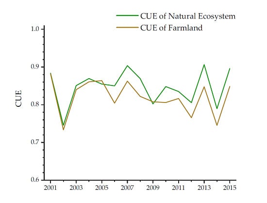
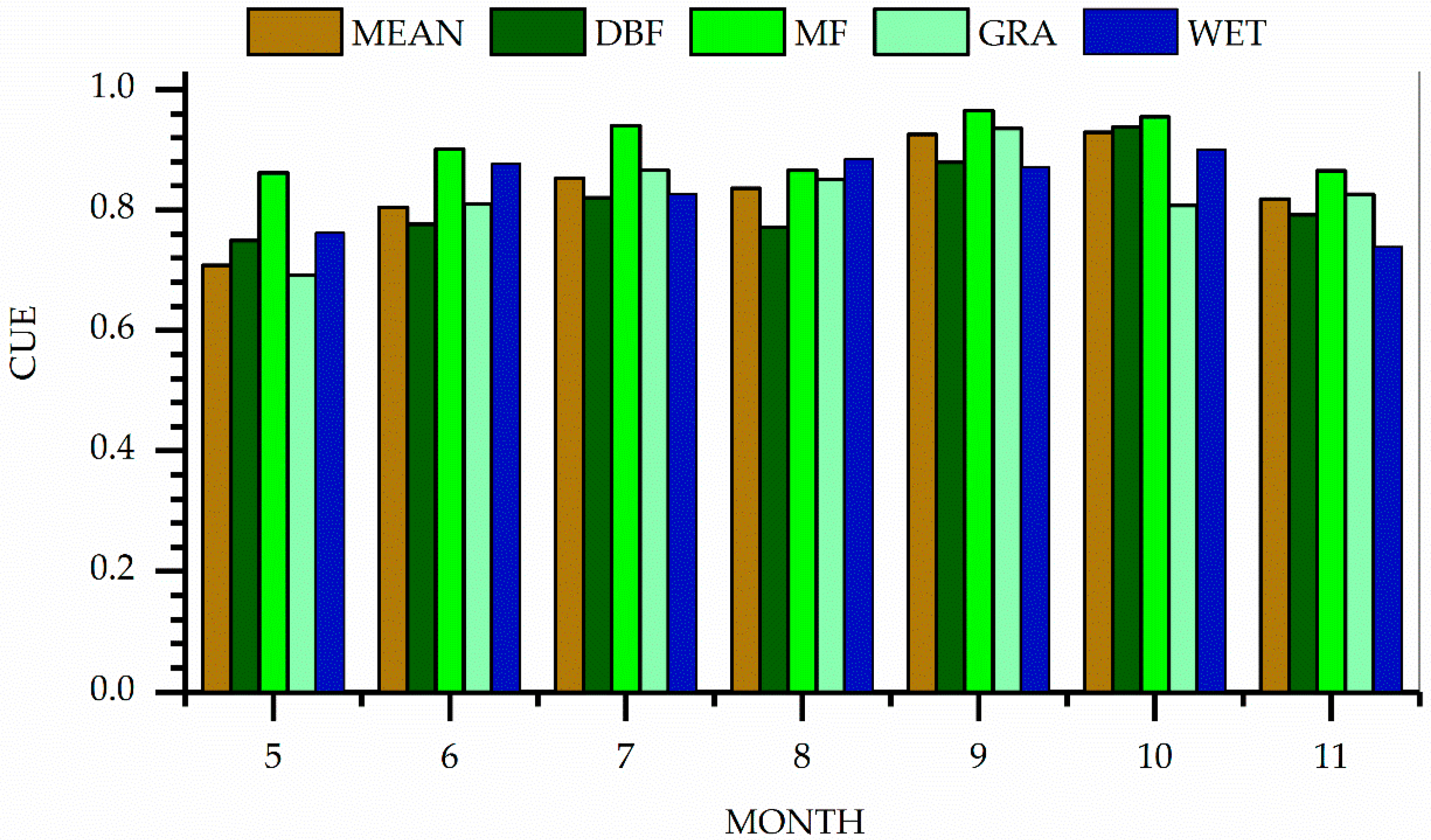
3.1. Monthly Change of CUE

The CUE value of natural ecosystems in the SNP started from May and continued to November, the CUE changed significantly within the year (Figure 3). The lowest CUE values occurred in May. After July, CUE increased, and exceeded 0.8. The highest CUE (over 0.9) values were mainly observed in October. The growing season started in May in SNP with low NPP and carbon sequestration capacity. In contrast, the proportion of GPP increased in October after self-consumption through the growing season. The CUE of the natural ecosystems was higher after July, along with the accumulation of more NPP, which meant that the natural ecosystem protection capacity may be stronger.
There were three abnormally low CUE values in the SNP during the past 15 years (Figure 3). These were November 2002, May 2012 and October 2014. According to field-based meteorological measurements, the average temperature in November 2002 was the lowest in 15 years, which might be the reason that led to decrease in both GPP and NPP. In May 2012 and October 2014, the low CUE values might be associated with lower GPP and NPP due to reduced rainfall in those months.
The monthly CUE varied among different ecosystems in the SNP (Figure 4). Except for May and October, the CUE of DBF was generally lower than the regional monthly average, while the GRA was the opposite. GRA started with a green-up in May and gradually entered a senescence period in October. GRA might produce more net productivity in those two months. The CUE of MF was always higher than the regional CUE average. WET CUE in May, June and August were greater than the CUE mean value. WET CUE was the highest in August, indicating that the proportion of GPP kept by WET ecosystems after self-consumption was the greatest.
The CUE of MF was the highest from May to November except for August. Compared to other ecosystems, MF may have stronger ecological protection effects. Due to higher temperature in August, CUE of GRA may be restricted, while the area covered by humid MF could produce a higher CUE. From June to August, CUE of DBF was the lowest, because the accumulated NPP was relatively lower than other types.

3.2. Seasonal Changes in CUE

Considering the dormancy of vegetation in the SNP in the winter months from December to the following February, we calculated CUE in spring (March to May), summer (June to August) and autumn (September to November), respectively. Figure 5 shows the seasonal variation of ecosystem CUE. The regional average CUE was 0.236, 0.835 and 0.854 in spring, summer and autumn, respectively. The highest and lowest CUEs in spring were observed in the year of 2013 (0.299) and 2012 (0.075), respectively. The lowest value of CUE in spring 2012 may be due to the drought of that year [26]. The maximum summer CUE (0.916) was observed in 2004, whereas the minimum value (0.75) occurred in 2011. CUE in autumn reached the peak (0.974) in 2011, while the lowest value was found in 2014 (0.686).
In most years, average CUE was the lowest in spring. The average CUE values in summer of 2002, 2009, and 2014 were greater than those in autumn, which was related to successive drought from summer to autumn. It was found that the degree of CUE decrease depends not only on the intensity of the drought, but also the duration of the drought intensity and the time of occurrence [27].
Spatially, spring CUE in the southwest of the SNP was higher than the east during the 15 years (Figure 6). It ranged from 0 to 0.4, with an average value of 0.24 (Figure 6a). In summer, vegetation grew vigorously, and the carbon sequestration capacity of vegetation increased (Figure 6b). Similar spatial distribution pattern was observed in summer with an average CUE of 0.83. With the arrival of autumn, the CUE in most regions also increased and ranged from 0.8 to 1.0 with an average value of 0.88 (Figure 6c). In summer and autumn, the carbon sequestration capacity of natural ecosystems was better, indicating the relatively stronger ecological protection function.
In terms of spatial distribution, the pixels showing an upward trend in three seasons were mainly found in grasslands in the southwest and deciduous broadleaf forest in the eastern fringe. According to the slope analysis, about two-thirds of the study area showed an upward trend of CUE in spring (Figure 7a). CUE in summer tended to increase in 53.7% of the study area (Figure 7b), while the CUE showed increasing trend in the area of 56.7% in autumn (Figure 7c). This increasing trend suggested that the carbon sequestration capacity of natural ecosystem in the SNP could be improving. More NPP accumulated in natural ecosystem may make their ecological protection function stronger. The change trends of CUE (over 90% pixels) passed the significance level test at p < 0.05.
The seasonal changes of CUE for different ecosystems CUE were also obviously changing in the SNP (Figure 8). In spring, all types of vegetation had low CUE values (Figure 8a). Relatively good hydrothermal conditions in summer were more favorable to vegetation growth and the CUE of each vegetation type was generally increasing (Figure 8b). In autumn, CUE of MF, DBF and GRA continued to rise, whereas WET CUE declined slightly (Figure 8c). Among different ecosystems, CUE of MF had been the highest (spring: 0.288; summer: 0.902; autumn: 0.928).

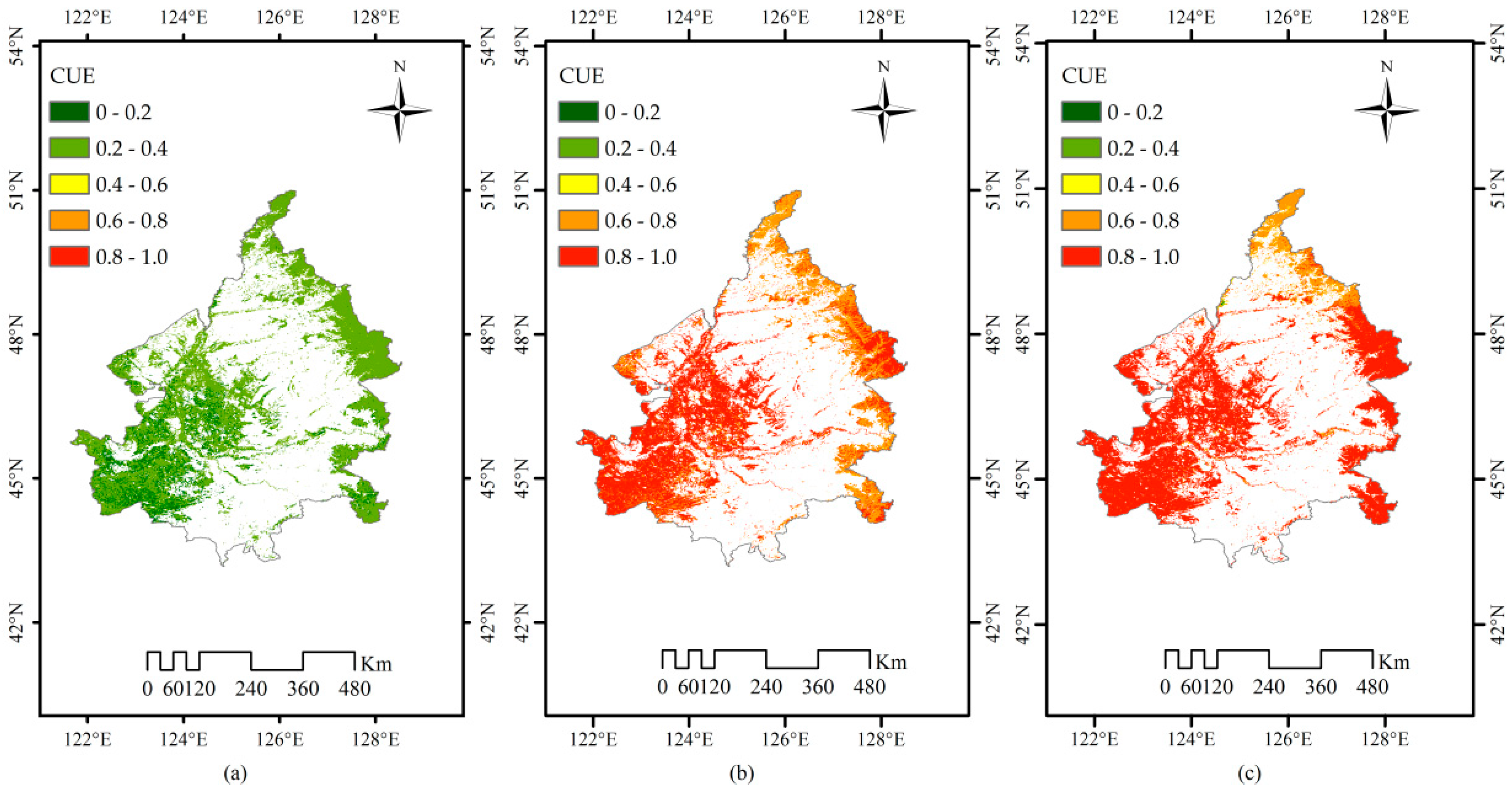
3.3. The Mean Spatial Distribution of LSP

Spatial distributions of LSP parameters, i.e., SOS, LOS and EOS, in the SNP from 2001 to 2015 are illustrated in Figure 9. The SOS of the natural ecosystem mainly occurred at day of year (DOY) between 100 and 150. The earliest SOS was found in the eastern parts of the SNP region, while the southwestern region had the latest SOS (Figure 9a). The growing season of DBF and MF started from mid-March, and GRA and WET had later start of the growing season (early April). SOS began in March and April, the vegetation began to accumulate GPP, but the CUE value was in a very small range, almost neglected, so we began to record CUE from May.
The distribution of EOS dates showed similar pattern to that of SOS, gradually increasing from west to east, mainly in late October and November (290–330 DOY) (Figure 9b). The end dates of the growing season of DBF and MF occurred in early November. GRA and WET ended their growing seasons about ten days earlier than the forestland. During 2001–2015, the average LOS of natural ecosystems in the SNP was about 192 days, showing similar spatial distribution to SOS and EOS (Figure 9c). The average LOS of MF and GRA was 213 days and 176 days, respectively. LOS dates of DBF were about 5 days shorter than those of MF, and the growing season of WET was about 4 days longer than that of GRA.

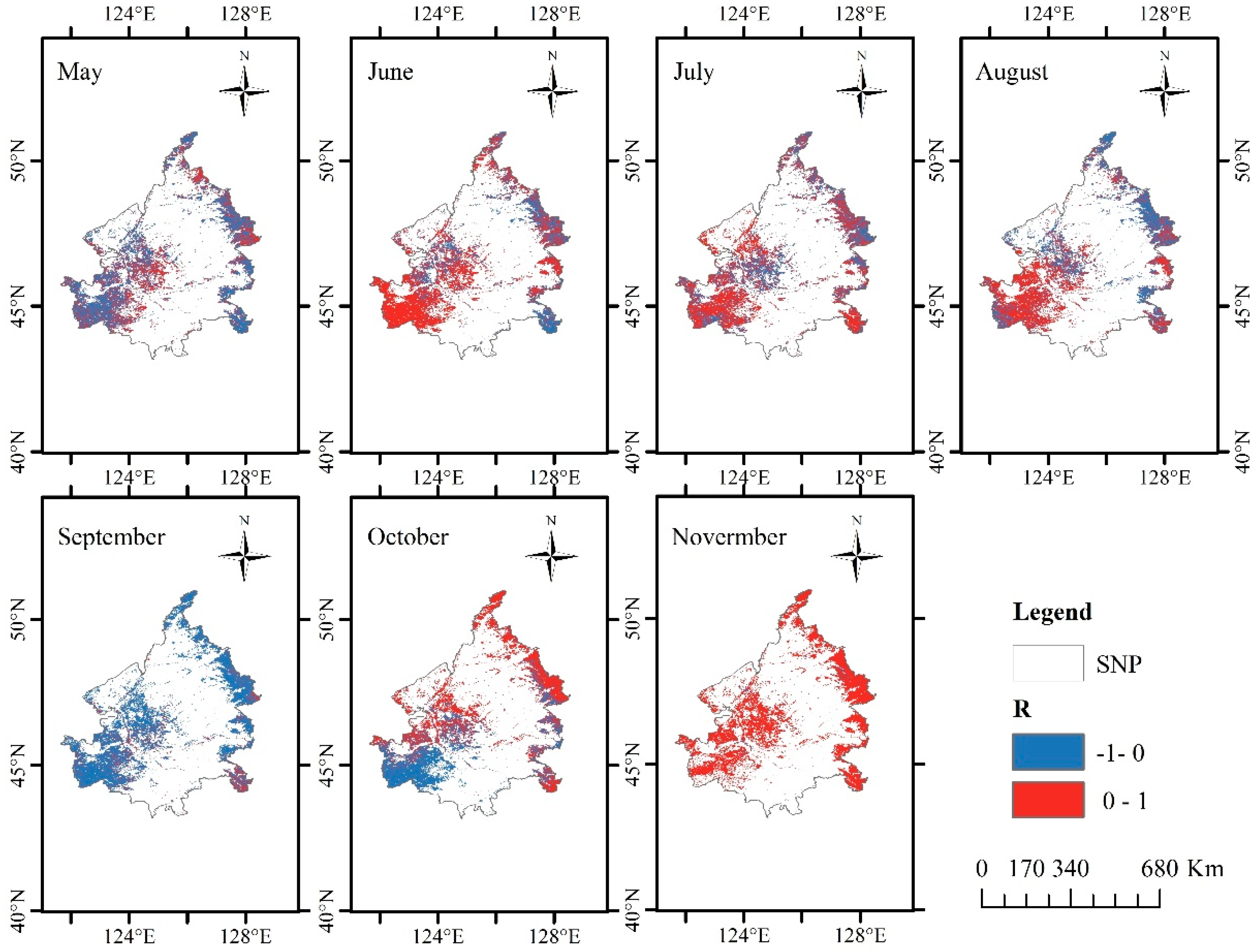
3.4. Response of CUE to LSP Variation

After analyzing the correlation between CUE and LSP in the growing seasons, it was found that CUE was negatively correlated with SOS in about 70% of the study area (Figure 10a and Figure 11). This indicated that earlier SOS would encourage higher CUE. In 72% of areas covered by GRA, CUE was negatively correlated with SOS. In 67% of the SNP, the later EOS would result in higher CUE. In 80% of areas covered by DBF, late EOS dates might have the positive effect on the increase of CUE (Figure 10b). CUE was positively correlated with LOS in more than 70% of areas covered by DBF, GRA and WET. The average CUE of MF with the longest growing season was highest (0.529). GRA with the second longest growing season (0.482). Although the LOS of GRA was the shortest, its average CUE (0.482) was greater than that of DBF (0.477). This would be because GRA in cold and dry regions consumed less energy to maintain growth. The area proportions of correlation coefficients after significant test for all the pixels were obtained (Figure 11).

3.5. Direct Effects of Local Climate Factors on CUE Change

This study revealed that a partial correlation existed between mean temperature and total precipitation and CUE in the growing season. CUE was negatively correlated with precipitation accounting for about 46.8% of the total pixels (Figure 12a). Among those, 0.98% had significant negative correlation, mainly distributed in the eastern and southwestern fringe areas of SNP. The area showing positive correlation between CUE of DBF and precipitation occupied 61.8% of the total area. About 60% of CUE values of GRA and WET were positively related to precipitation. CUE was positively affected by temperature in more than 90% of the region, of which 14.85% showed a significant positive correlation. Only in the northern and southern margins, CUE decreased with increasing temperature (Figure 12b).
At monthly scale, the responses of ecosystem CUE to climate drivers were also significantly different. Figure 13 and Figure 14 showed the spatial pattern of correlation coefficients between monthly CUE, precipitation and temperature from 2001 to 2015. Overall, the pixels with a positive correlation coefficient took up higher area proportions of the study area. Except for November, increased precipitation could contribute to higher CUE for the corresponding months in more than 60% of naturally vegetated area in the SNP (Figure 13 and Table 2). From June to August, CUE in more than 50% of pixels in the natural ecosystem had a positive correlation with temperature. On the other hand, as temperature increased, plant ecosystem might suffer higher ecosystem respiration cost and lower net productivity. In May and September, the pixels showing negative correlation coefficient between temperature and CUE occupied most of the SNP (Figure 14 and Table 3).

4. Discussion

Previous studies on CUE using remote sensing methods mainly focus on changes at annual scale. In this paper, CUE at the seasonal and monthly scales were investigated. Thus, the change trends of CUE and the climate factors affecting CUE in different growth stages could be explained. CUE was considered to be a constant value regardless of ecosystem types or species [28,29]. However, this assumption at a global scale might be controversial, because it ignores the influence of environmental factors [30,31]. Tang et al. [3] estimated global average CUE using site data, which varied widely between 0.201 and 0.822. In this study, the estimated monthly CUE from satellite observations ranged from 0.021 to 0.999 in the SNP. The results suggested that CUE among ecosystems could not be a constant. The assumption of a constant CUE of 0.5 might lead to biased estimates for carbon cycling modelling across temporal-spatial scales.
We compared the CUE calculated by the same model of different ecosystems at the annual scale from other reported studies (Table 4). The order of annual CUE of different ecosystems in SNP was as follows: GRA (0.567) > WET (0.542) > MF (0.480) > DBF (0.479) [19]. Tang et al. [3] found the largest CUE for WET on a global scale. Khalifa et al. [32] estimated the CUE of different vegetation in sub Saharan area and found that the annual average CUE deceased in the following sequence: WET > GRA > MF > DBF. However, in our study, the order of average CUE of the growing season in the SNP was: MF > WET > GRA > DBF. This difference may be due to the different time scales and regions with of the studies.
Previous studies indicated that plant CUE might demonstrate a significant seasonal variation. In the short term, such as over one year, the dynamic patterns of carbohydrate storage and plant carbon allocation may lead to great changes in CUE [33]. Campioli et al. [7], using biometric methods and vortex correlation techniques, evaluated temporal and spatial variation of CUE in Fagus sylvatica forest and found that CUE in spring was the highest. Artificially grown apples have higher CUE in summer, which may be consistent with the higher accumulation of biomass and the lower respiratory consumption [34]. In contrast, as SNP is at mid-high latitudes, vegetation in the SNP may reduce the consumption of respiration and increase the carbon sequestration capacity in autumn, leading to the highest CUE.
CUE is regarded as a dynamic parameter, and differs among species of the same biome [35]. In this study, we found that the CUE of MF ecosystems in the SNP had great potential for carbon sequestration in different seasons. GPP and NPP of GRA were very small in spring, resulting in the lowest CUE. In summer and autumn, the CUE of GRA gradually increased. This study found that CUE of GRA in summer was higher than that of DBF, possibly because GRA had less investment in plant tissue respiration than that of broad-leaved forest, as reported by Law et al. [36]. Forest types showed high CUE in autumn, because trees with higher carbon storage might be more beneficial to the growth in the next year. After analyzing the abnormal values of different vegetation in different years (Figure 8), this study found that in the spring of 2012, CUE of all types of vegetation decreased to the lowest level, which would be related to different degrees of spring drought occurring in the western part of the SNP region [26]. With lower average temperature in the autumn of 2002, CUE decreased in the SNP as the temperature decreased, along with the CUE value. In the autumn of 2014, the CUE of vegetation decreased significantly, which was associated with moderate drought in the south-central Northeast China [37].
Phenological records can not only directly reveal the changes of natural seasons, but also illustrate the response and adaptation of ecosystem process and results to global environmental changes. Few previous studies have discussed the relationship between phenology and CUE. The phenological metrics that we extracted were similar to the study of Huang et al. [2]. Most of the existing literatures have focused on the relationship between NPP, GPP and phenology. Earlier SOS may extend the growing season longer and lead to an increase in GPP [38]. Similarly, the delay in EOS may also prolong the growth season, causing increases in GPP and NPP [18]; therefore, the CUE value of the vegetation will increase. Vegetation requires relatively less energy to maintain living tissues in lower temperature conditions, resulting in less respiration costs and higher CUE [39]. On the other hand, vegetation growth is generally constrained by the short growing season. Rising temperature could extend the growing season length and significantly increase GPP [12]. The sensitivity of CUE to temperature under lower-temperature conditions is lower because the temperature sensitivities of GPP and autotrophic respiration are of comparable size. In warm regions, especially in the tropics where the growing season is long, by contrast, the respiration consumption of vegetation are higher, leading to a lower CUE [1].
CUE is sensitive to environmental conditions and climate change [40]. Previous studies found that net productivity would increase linearly with higher average annual precipitation and temperature in cold and dry ecosystem [1]. As a function of GPP, NPP and respiration, CUE of vegetation (for instance, forest) may be affected by temperature and precipitation [41]. One reported study suggested that CUE exhibited a decreasing trend with the increase of precipitation when precipitation was less than 2300 mm year–1. CUE showed an increasing trend along temperature when it was between −10 °C and 20 °C, as well as an increasing trend with rising temperature [1]. In this study, CUE showed an increasing trend from May to July and from August to October, respectively, possibly because the hydrothermal condition was more suitable during those two time periods. Increased precipitation may lead to a higher NPP/GPP ratio [6]. The variations of temperature affect both the photosynthesis and Ra rates, resulting in the changes of vegetation CUE [42]. The ratio of NPP to GPP might increase as the annual temperature increased between −10 and 20 °C [1], which was partially explained by the findings of this study.
In addition, in recent decades, to improve the local ecological environment and enhance the ecological protection barrier function, the Chinese government and local citizens have taken multiple measures and implemented actions for ecological and environmental protection [2]. Ecological and environmental restoration projects such as the “Three-North Shelterbelt Project” and the “Grain for Green Project” have achieved some positive effects [43,44]. We used the same method to calculate the CUE of farmland. By comparison, we found that the average CUE of the natural ecosystem in SNP showed a similar variation as that of the internal farmland from 2001 to 2015 (Figure 15). The CUE of farmland and natural ecosystem increased simultaneously. The respiration consumption of vegetation decreased. This also showed that the ecological protection function of natural ecosystem may have been strengthened during the past 15 years.

5. Conclusions

Quantifying the variations of interannual CUE among ecosystems has proved to be a useful tool when calculating interannual carbon budgets. However, the intraannual change of CUE may present different characteristics. The assessment of temporal and spatial variations of CUE at shorter time scales and the impact on them of phenological and climatic factors are still poorly understood. This study attempted to reveal spatial patterns of CUE of natural ecosystems at different temporal scales in the SNP, China. The differences of CUE between months and seasons were significant. Monthly average CUE showed the highest in October and lowest in May. Average CUE was the highest in autumn, followed by summer. The variability of NPP accumulation in different seasons was significant. The highest CUE values were observed in MF in the growing season, indicating better ecological protection effects. The spatial variations of CUE were different. The pixels with rising CUE were mainly concentrated in southwest GRA and eastern DBF. The SOS was generally observed in March and April, while EOS dates were found in October and November. The earlier SOS and later EOS exerted a positive influence on CUE in the SNP, especially in 80% of the areas covered by broad-leaved forest. Longer LOS might cause the increase in CUE. In addition, CUE was positively correlated with precipitation and temperature in most areas of the SNP. Increasing trend of CUE in the SNP suggested a protective barrier function of natural ecosystems in the protected farmland region.

Author Contributions

B.L. and F.H. had the original idea for the study and designed the research. B.L. analyzed the data and wrote the paper. F.H. supervised the research and provided significant suggestions. L.Q., H.Q. and N.S. was involved in the data processing and the manuscript reviewing.

Funding

This research was supported by the National Natural Science Foundation of China (Grant No. 41571405 and 41571115) and the key project of the National Natural Science Foundation of China (Grant No. 41630749).

Acknowledgments

The authors would like to thank the reviewers and editors for their valuable comments and suggestions.

Conflicts of Interest

The authors declare no conflict of interest.

References

  1. Zhang, Y.; Xu, M.; Chen, H.; Adams, J. Global pattern of NPP to GPP ratio derived from MODIS data: Effects of ecosystem type, geographical location and climate. Glob. Ecol. Biogeogr. 2009, 18, 280–290. [Google Scholar] [CrossRef]
  2. Huang, F.; Wang, P.; Chang, S.; Li, B. Rain use efficiency changes and its effects on land surface phenology in the Songnen Plain, Northeast China. In Proceedings of the SPIE Remote Sensing 2018, Berlin, Germany, 11–12 September 2018. [Google Scholar] [CrossRef]
  3. Tang, X.; Carvalhais, N.; Moura, C.; Ahrens, B.; Koirala, S.; Fan, S.; Guan, F.; Zhang, W.; Gao, S.; Magliulo, V.; et al. Global variability of carbon use efficiency in terrestrial ecosystems. Biogeosci. Discuss. 2019, 2019. [Google Scholar] [CrossRef]
  4. Delucia, E.; Drake, J.; Thomas, R.; Gonzalez, M. Forest carbon use efficiency: Is respiration a constant fraction of gross primary production? Glob. Chang. Biol. 2007, 13, 1157–1167. [Google Scholar] [CrossRef]
  5. Luyssaert, S.; Inglima, I.; Jung, M.; Richardson, A.; Reichsteins, M.; Papale, D.; Piao, S.; Schulzes, E.; Wingate, L.; Matteucci, G. CO2 balance of boreal, temperate, and tropical forests derived from a global database. Glob. Chang. Biol. 2007, 13, 2509–2537. [Google Scholar] [CrossRef]
  6. Zhang, Y.; Yu, G.; Jian, Y.; Wimberly, M.; Zhang, X.; Jian, T.; Jiang, Y.; Zhu, J. Climate-driven global changes in carbon use efficiency. Glob. Ecol. Biogeogr. 2014, 23, 144–155. [Google Scholar] [CrossRef]
  7. Campioli, M.; Gielen, B.; Gockede, M.; Papale, D.; Bouriaud, O.; Granier, A. Temporal variability of the NPP-GPP ratio at seasonal and interannual time scales in a temperate beech forest. Biogeosciences 2011, 8, 2481–2492. [Google Scholar] [CrossRef] [Green Version]
  8. Chambers, J.; Tribuzy, E.; Toledo, L. Rrepiration from a tropical forest ecosystem: Partitioning of sources and low carbon use efficiency. Ecol. Appl. 2004, 14, S72–S88. [Google Scholar] [CrossRef]
  9. Amthor, J. The McCree–de Wit–Penning de Vries–Thornley Respiration Paradigms: 30 Years Later. Ann. Bot. 2000, 86, 1–20. [Google Scholar] [CrossRef]
  10. Li, Y.; Fan, J.; Hu, Z.; Shao, Q.; Harris, W. Comparison of evapotranspiration components and water-use efficiency among different land use patterns of temperate steppe in the Northern China pastoral-farming ecotone. Int. J. Biometeorol. 2015, 60, 827–841. [Google Scholar] [CrossRef] [Green Version]
  11. Yu, G.; Wang, Q.; Zhuang, J. Modeling the water use efficiency of soybean and maize plants under environmental stresses: Application of a synthetic model of photosynthesis-transpiration based on stomatal behavior. J. Plant Physiology 2004, 161, 303–318. [Google Scholar] [CrossRef]
  12. Piao, S.; Wang, S. Forest annual carbon cost: A global-scale analysis of autotrophic respiration. Ecology 2010, 91, 652–661. [Google Scholar] [CrossRef] [PubMed]
  13. He, Y.; Piao, S.; Li, X.; Chen, A.; Qin, D. Global patterns of vegetation carbon use efficiency and their climate drivers deduced from MODIS satellite data and process-based models. Agric. For. Meteorol. 2018, 256, 150–158. [Google Scholar] [CrossRef]
  14. Noormets, A. (Ed.) Phenology of Ecosystem Processes; Springer: New York, NY, USA, 2009. [Google Scholar] [CrossRef]
  15. Richardson, A.; Keenan, T.; Migliavacca, M.; Ryu, Y.; Sonnentag, O.; Toomey, M. Climate change, phenology, and phenological control of vegetation feedbacks to the climate system. Agric. For. Meteorol. 2013, 169, 156–173. [Google Scholar] [CrossRef]
  16. Jin, J.; Ying, W.; Zhen, Z.; Magliulo, V.; Min, C. Phenology plays an important role in the regulation of terrestrial ecosystem water-use efficiency in the Northern Hemisphere. Remote Sens. 2017, 9, 664. [Google Scholar] [CrossRef]
  17. Min, M.; Zhu, W.; Wang, W.; Xu, Y.; Liu, J. Evaluation of vegetation phenology remote sensing identification method based on carbon exchange data of flux tower net ecosystem. Chin. J. Appl. Ecol. 2012, 23, 319–327. [Google Scholar]
  18. Qi, H.; Huang, F.; Zhai, H. Monitoring spatio-temporal changes of terrestrial ecosystem soil water use efficiency in Northeast China using time series remote sensing data. Sensors 2019, 19, 1481. [Google Scholar] [CrossRef]
  19. Li, B.; Huang, F.; Chang, S.; Sun, N. The variations of satellite-based ecosystem water use and carbon use efficiency and their linkages with climate and human drivers in the Songnen Plain, China. Adv. Meteorol. 2019, 2019, 8659138. [Google Scholar] [CrossRef]
  20. Huang, F.; Liu, X.; Wang, P.; Zhang, S.; Zhang, Y. Land use/cover change and its driving forces of west of Songnen Plain. J. Soil Water Conserv. 2003, 17, 14–17. [Google Scholar] [CrossRef]
  21. Piao, S.; Fang, J.; Guo, Q. Application of CASA model to the estimation of Chinese terrestrial net primary productivity. Acta Phytoecol. Sin. 2001, 25, 603–608. [Google Scholar] [CrossRef]
  22. Zhu, W.; Pan, Y.; He, H.; Yu, D.; Hu, H. Simulation of maximum light utilization rate of typical vegetation in China. Chin. Sci. Bull. 2006, 51, 700–706. [Google Scholar] [CrossRef]
  23. Mao, D.; Wang, Z.; Han, J.; Ren, C. Temporal and spatial patterns and driving factors of vegetation NPP in Northeast China from 1982 to 2010. Sci. Geogr. Sin. 2012, 32, 1106–1111. [Google Scholar]
  24. Tang, J.; Jiang, Y.; Zhang, N.; Hu, M. Estimation of vegetation net primary productivity and carbon sink in western jilin province based on CASA model. J. Arid Land Resour. Environ. 2013, 27, 1–7. [Google Scholar]
  25. Tang, X.; Li, H.; Desai, A.; Nagy, Z.; Luo, J.; Kolb, T.; Olioso, A.; Xu, X.; Li, Y.; Kutsch, W. How is water-use efficiency of terrestrial ecosystems distributed and changing on Earth? Sci. Rep. 2014, 4, 7483. [Google Scholar] [CrossRef] [PubMed]
  26. Wang, S.; Duan, H.; Feng, J. Drought events and its influence in spring of 2012 in China. J. Arid Meteorol. 2012, 30, 298–304. [Google Scholar] [CrossRef]
  27. George, L. Carbon-use efficiency of terrestrial ecosystems under stress conditions in Southeast Europe (MODIS, NASA). Proceedings 2018, 2, 363. [Google Scholar] [CrossRef]
  28. Running, S. A general model of forest ecosystem processes for regional applications I. Hydrologic balance, canopy gas exchange and primary production processes. Ecol. Model. 1988, 42, 125–154. [Google Scholar] [CrossRef]
  29. Gifford, R. The global carbon cycle: A viewpoint on the missing sink. Funct. Plant Biol. 1994, 21, 1–15. [Google Scholar] [CrossRef]
  30. Dewar, R.; Medlyn, B.; Mcmurtrie, R. Acclimation of the respiration/photosynthesis ratio to temperature: Insights from a model. Glob. Chang. Biol. 2010, 5, 615–622. [Google Scholar] [CrossRef]
  31. Xiao, C.; Yuste, J.; Janssens, I.; Roskams, P.; Nachtergale, L.; Carrara, A.; Sanchez, B.Y.; Ceulemans, R. Above- and belowground biomass and net primary production in a 73-year-old scots pine forest. Tree Physiol. 2003, 23, 505–516. [Google Scholar] [CrossRef]
  32. Khalifa, M.; Elagib, N.; Ribbe, L.; Schneider, K. Spatio-temporal variations in climate, primary productivity and efficiency of water and carbon use of the land cover types in Sudan and Ethiopia. Sci. Total Environ. 2018, 624, 790–806. [Google Scholar] [CrossRef]
  33. Arneth, A.; Kelliher, F.; McSeveny, T.; Byers, J. Net ecosystem productivity, net primary productivity and ecosystem carbon sequestration in a pinus radiata plantation subject to soil water deficit. Tree Physiol. 1998, 18, 785. [Google Scholar] [CrossRef] [PubMed]
  34. Zanotelli, D.; Montagnani, L.; Manca, G.; Tagliavini, M. Net primary productivity, allocation pattern and carbon use efficiency in an apple orchard assessed by integrating eddy-covariance, biometric and continuous soil chamber measurements. Biogeosciences 2013, 10, 3089–3108. [Google Scholar] [CrossRef]
  35. Street, L.E.; Subke, J.A.; Sommerkorn, M.; Sloan, V.; Ducrotoy, H.; Phoenix, G.K.; Williams, M. The role of mosses in carbon uptake and partitioning in arctic vegetation. New Phytol. 2013, 199, 163–175. [Google Scholar] [CrossRef] [PubMed]
  36. Law, B.; Falge, E.; Gu, L.; Baldocchi, D.; Bakwin, P.; Berbigier, P.; Davis, K.; Dolman, A.; Falk, M.; Fuentes, J. Environmental controls over carbon dioxide and water vapor exchange of terrestrial vegetation. Agric. For. Meteorol. 2015, 113, 97–120. [Google Scholar] [CrossRef]
  37. Wang, S.; Duan, H.; Feng, J. Drought events and its influence in autumn of 2014 in China. J. Arid Meteorol. 2014, 32, 1031–1039. [Google Scholar] [CrossRef]
  38. Keenan, T.; Gray, J.; Friedl, M.; Toomey, M.; Bohrer, G. Net carbon uptake has increased through warming-induced changes in temperate forest phenology. Nat. Clim. Chang. 2014, 4, 598–604. [Google Scholar] [CrossRef]
  39. Ryan, M.; Linder, S.; Vose, J.; Hubbard, R. Dark respiration of pines. Ecol. Bull 1994, 43, 50–63. [Google Scholar] [CrossRef]
  40. Bradford, M.; Crowther, T. Carbon use efficiency and storage in terrestrial ecosystems. New Phytol. 2013, 199, 7–9. [Google Scholar] [CrossRef]
  41. Cox, P. Description of the “Triffid” Dynamic Global Vegetation Model. Hadley Centre Technical Note. 2001. Available online: https://www.researchgate.net/publication/245877262_Description_of_the_TRIFFID_dynamic_global_vegetation_model/related (accessed on 26 October 2019).
  42. Giardina, C.P.; Ryan, M.G.; Binkley, D.; Fownes, J.H. Giardina, Primary production and carbon allocation in relation to nutrient supply in a tropical experimental forest. Glob. Chang. Biol. 2003, 9, 1438–1450. [Google Scholar] [CrossRef]
  43. Li, A.; Han, Z.; Huang, C.; Tan, Z. Remote sensing monitoring on dynamic of sandy desertification degree in Horqin sandy land at the beginning of 21st century. J. Desert Res. 2007, 27, 546–551. [Google Scholar]
  44. Du, Z.; Zhan, Y.; Wang, C.; Song, G. The dynamic monitoring of desertification in Horqin sandy land on the basis of MODIS NDVI. Remote Sens. Land Resour. 2009, 21, 14–18. [Google Scholar] [CrossRef]
Figure 1. Study Area. FL: farmland; DBF: deciduous broad-leaved forest; MF: mixed forest; GRA: grassland and WET: wetland.
Remotesensing 11 02513 g001
Figure 2. The flow chart of the research approach.
Remotesensing 11 02513 g002
Figure 3. Regional average CUE at the monthly scale from 2001 to 2015.
Remotesensing 11 02513 g003
Figure 4. Monthly mean CUE of different ecosystems from 2001 to 2015.
Remotesensing 11 02513 g004
Figure 5. Average CUE variations in spring, summer and autumn from 2001 to 2015.
Remotesensing 11 02513 g005
Figure 6. Spatial distribution of seasonal average CUE of the SNP from 2001 to 2015. (a) Spring; (b) summer; (c) autumn.
Remotesensing 11 02513 g006
Figure 7. Spatial trend of average CUE in each season of SNP from 2001 to 2015. (a) Spring; (b) summer; (c) autumn.
Remotesensing 11 02513 g007
Figure 8. CUE of different ecosystems and seasons from 2001 to 2015. (a) Spring; (b) summer; (c) autumn.
Remotesensing 11 02513 g008
Figure 9. Spatial distribution of land surface phenology metrics in the SNP from 2001 to 2015: (a) average SOS; (b) average EOS; (c) average LOS.
Remotesensing 11 02513 g009
Figure 10. Spatial distribution of correlation coefficients (R) between CUE, SOS, EOS and LOS in the SNP during 2001–2015. (a) CUE and SOS; (b) CUE and EOS; (c) CUE and LOS.
Remotesensing 11 02513 g010
Figure 11. The area percentages of correlation coefficients between CUE, SOS, EOS and LOS. (Significant Positive Correlation (r > 0, p < 0.05): No Significant Positive Correlation (r > 0, p > 0.05), No Significant Negative Correlation (r < 0, p > 0.05), Significant Negative Correlation (r < 0, p < 0.05)).
Remotesensing 11 02513 g011
Figure 12. Partial correlation coefficients between CUE and major climatic factors in the growing season: (a) precipitation; (b) temperature.
Remotesensing 11 02513 g012
Figure 13. Correlation coefficients between CUE and monthly precipitation.
Remotesensing 11 02513 g013
Figure 14. Correlation coefficients between CUE and temperature at monthly scale during 2001–2015.
Remotesensing 11 02513 g014
Figure 15. Average CUE variations of natural ecosystems and farmland in the SNP from 2001 to 2015.
Remotesensing 11 02513 g015
Table 1. Description of the data used in this study.
DatasetSourceTemporal ResolutionTime RangeSpatial Resolution
GPPMOD178-day composite2001–20151 km
Land coverMCD12Q1annual2001–20151 km
NDVIMOD1316-day composite2001–20150.25 km
Temperaturehttp://data.cma.cn/monthly2001–2015/
Precipitationhttp://data.cma.cn/monthly2001–2015/
Solar radiationhttp://data.cma.cn/monthly2001–2015/
Table 2. The number of pixels and their proportions of correlation coefficients between monthly precipitation and CUE.
MonthPositive Pixels (%)Negative Pixels (%)
May67,293 (91.60%)6170 (8.40%)
June58,717 (79.93%)14,746 (20.07%)
July49,180 (66.95%)24,283 (33.05%)
August61,691 (83.98%)11,772 (16.02%)
September69,366 (94.42%)4097 (5.58%)
October44,115 (60.05%)29,348 (39.95%)
November20,398 (27.77%)53,065 (72.23%)
Table 3. The number of pixels and their proportions of the correlation coefficients between monthly temperature and CUE.
MonthPositive Pixels (%)Negative Pixels (%)
May25,181 (34.28%)48,282 (65.72%)
June48,525 (66.05%)24,938 (33.95%)
July43,585 (59.33%)29,878 (40.67%)
August39,588 (53.89%)33,875 (46.11%)
September7667 (10.44%)65,796 (89.56%)
October38,603 (52.55%)34,860 (47.45%)
November72,078 (98.11%)1385 (1.89%)
Table 4. Comparison of estimated CUE at different time scales in different researches.
EcosystemTime ScaleCUEScaleType of DataData Source
WETAnnual0.607 ± 0.133GlobalSite dataTang [3]
Annual0.550–0.60Sudan and EthiopiaRemote sensing dataKhalifa [32]
Annual0.542SNPRemote sensing dataLi [19]
Growing season0.488SNPRemote sensing dataOur article
GRAAnnual0.457 ± 0.109GlobalSite dataTang
Annual0.220–0.560Sudan and EthiopiaRemote sensing dataKhalifa
Annual0.567SNPRemote sensing dataLi
Growing season0.482SNPRemote sensing dataOur article
MFAnnual0.464 ± 0.127GlobalSite dataTang
Annual0.350–0.480Sudan and EthiopiaRemote sensing dataKhalifa
Annual0.480SNPRemote sensing dataLi
Growing season0.530SNPRemote sensing dataOur article
DBFAnnual0.464 ± 0.127GlobalSite dataTang
Annual0.340–0.420Sudan and EthiopiaRemote sensing dataKhalifa
Annual0.479SNPRemote sensing dataLi
Growing season0.477SNPRemote sensing dataOur article

