The Temporal Dynamics of Slums Employing a CNN-Based Change Detection Approach


Faculty of Geo-Information Science and Earth Observation (ITC), University of Twente, 7514 AE Enschede, The Netherlands
*
Author to whom correspondence should be addressed.
Remote Sens. 2019, 11(23), 2844; https://doi.org/10.3390/rs11232844
Submission received: 19 October 2019
/
Revised: 15 November 2019
/
Accepted: 23 November 2019
/
Published: 29 November 2019
(This article belongs to the Special Issue Remote Sensing-Based Urban Planning Indicators)
Abstract
:Along with rapid urbanization, the growth and persistence of slums is a global challenge. While remote sensing imagery is increasingly used for producing slum maps, only a few studies have analyzed their temporal dynamics. This study explores the potential of fully convolutional networks (FCNs) to analyze the temporal dynamics of small clusters of temporary slums using very high resolution (VHR) imagery in Bangalore, India. The study develops two approaches based on FCNs. The first approach uses a post-classification change detection, and the second trains FCNs to directly classify the dynamics of slums. For both approaches, the performances of 3 × 3 kernels and 5 × 5 kernels of the networks were compared. While classification results of individual years exhibit a relatively high F1-score (3 × 3 kernel) of 88.4% on average, the change accuracies are lower. The post-classification results obtained an F1-score of 53.8% and the change-detection networks obtained an F1-score of 53.7%. According to the trajectory error matrix (TEM), the post-classification results scored higher for the overall accuracy but lower for the accuracy difference of change trajectories than the change-detection networks. Although the two methods did not have significant differences in terms of accuracy, the change-detection network was less noisy. Within our study area, the areas of slums show a small overall decrease; the annual growth of slums (between 2012 and 2016) was 7173 m2, in contrast to an annual decline of 8390 m2. However, these numbers hid the spatial dynamics, which were much larger. Interestingly, areas where slums disappeared commonly changed into green areas, not into built-up areas. The proposed change-detection network provides a robust map of the locations of changes with lower confidence about the exact boundaries. This shows the potential of FCNs for detecting the dynamics of slums in VHR imagery.

1. Introduction
Presently, more than half of the world’s population resides in urban settlements, with an expected increase to 68% by 2050 [1]. However, the lack of cities’ capacity to meet this sharply increasing housing demand, combined with the inability to provide basic services, drives the growth and persistence of slums [2]. The definitions of slums vary across the world. A globally commonly used definition by UN-Habitat defines a slum by the lack of one or more of the following: Durable housing, sufficient living space, easy access to safe water, access to adequate sanitation, and security of tenure [3]. Upgrading slums to ensure access to adequate and affordable housing and basic services has become one of the targets (indicator 11.1.1) in realizing the Sustainable Development Goals (SDGs) by the United Nations [4]. Slum maps provide information about the spatial characteristics of slum locations, extents, and structures. Assisted by a slum map, local authorities can improve infrastructures and basic services in slums [5]. With the advances in remote sensing technology, satellite imagery has become an important data source for producing slum maps. Image-based conceptualization of slums often refers to building characteristics, such as roof materials, shape, and density [6]. Such characteristics can be used for slum identification from remote sensing imagery. With these physical characteristics, slums can be detected and monitored. Such maps provide consistent and easily updateable slum information compared with that of a national census, knowing that census data are often very uncertain, quickly outdated, and usually cover only parts of the slums [7].
There are three primary study purposes of slum mapping based on remote sensing methods: Where, when, and what [6]: “Where” is about the location of slums in an urban region, “when” is to measure the temporal changes of slums, and “what” is related to questions such aspects as the populations of slums. Unlike the other two aspects, only a few studies have been performed to analyze “when”, i.e., the temporal dynamics of slums [8,9]. One reason for the lack of such studies is the availability of data [6], as well as the complexity of producing change-detection results [10]. For example, changes captured might refer to real change or pixel differences caused by variations in image conditions (e.g., along the boundaries of slums). A further issue relates to the transferability of mapping methods across multi-temporal images. Transferability is the ability to transfer the method or algorithm developed in one image to another image and achieving comparable mapping accuracies [11].
Researchers have been working on various approaches for slum identification based on VHR imagery, including texture analysis [12], object-based image analysis [13,14,15], landscape analysis [16], machine learning [17] with increasing attention on deep-learning [18,19,20], and recently, combining Object-Based Image Analysis (OBIA) and deep learning [21]. To map temporal dynamics, no conclusion on the best method exists; while OBIA-based method showed limitations in mapping trajectories [10], deep-learning-based methods have not been much explored for mapping the dynamics of slums. Convolutional Neural Networks (CNNs), which are a specific technique in the machine learning field, have drawn increasing attention in solving remote sensing classification tasks and show promising accuracies for slum mapping [6,21]. In the last decade, CNNs have been increasingly used in the analysis of remote sensing imagery e.g., [22,23,24,25]. For slum mapping, both CNNs [24] and fully convolutional networks (FCNs) [26] showed promising results with overall accuracies of over 80%. Fully convolutional networks (FCNs) are a particular architecture of CNNs designed for semantic image segmentation (pixel-wise classification) [27]. By replacing the fully connected layers in a CNN architecture with a convolution layer, FCNs maintain the structure of the original image [28]. Unlike CNNs, in which the output must be the same size as the input, FCNs allow the taking of images of any size as input [29]. A recent study [26] has shown that slums can be effectively detected in very high resolution (VHR) images by FCN techniques. So far, FCNs have not been used for analyzing the temporal dynamics of slums. Therefore, this study analyzes the potential of transferring an FCN-based classifier trained to identify slums to multi-temporal VHR images. Specifically, this study aims to explore the potential of FCNs to analyze the temporal dynamics of temporary (and in general very small) slum areas based on very high resolution (VHR) imagery in Bangalore, India. The study proposes two FCN-based approaches to generate slum change maps and assesses their performance. For one approach, slum maps from the land cover classification results are used for post-classification change detection. For the second approach, the FCNs are used to directly classify the changed slum areas in the imagery.
2. Materials and Methods
The methodology of this research starts with the preparation and pre-processing of the data, including the selection of study tiles and the preparation of reference data. Then, two approaches for applying FCNs were employed to capture the temporal dynamics of slums in the study area. The first approach applied FCNs to classify temporary slums and other land uses for each year. Followed by a post-classification change-detection process, the changes in slum areas were extracted from the individual land-use classifications. The second approach used FCNs to directly detect the changed slum areas over two years. After the changed areas were captured, in a next step, the accuracy was assessed using both a confusion matrix and a trajectory error matrix. Finally, the temporal dynamics of the slums are analyzed and discussed.
2.1. The Study Area and Data Sets
Bangalore is one of the biggest cities in India, housing more than 8 million people in its metropolitan area [30]. The India census in 2011 reported that around 8.39% of the total population in the city of Bangalore is living in slums [31]. However, a recent study suggested that every fifth person in the city of Bangalore lives in a slum [32]. This difference is mainly caused by the different definitions of slums, and the exclusion of temporary slums (e.g., homes of migrant workers) in official statistics. For example, India also sets a minimum settlement size for an area to be considered as a slum, requiring at least 300 people or 60–70 households living in a settlement cluster [33]. Thus, there are two types of slums: Notified slums and non-notified slums. Notified slum dwellers can usually afford to invest in education and skill training, while residents in non-notified slums are mostly unconnected to basic services and formal livelihood opportunities [34]. Krishna [34] also categorized non-notified slums in Bangalore into three types: New migrants, very low-income settlements, and low-income settlements. In this hierarchy, “New Migrants” indicates a shelter type typically characterized by blue plastic sheeting and small unit size (Figure 1). People living in these shelters are typically not covered by any official information, but require basic services [34]. Furthermore, temporary slums are commonly very small in area size (mean area size is 719 m2, compared to all slums in Bangalore with a mean size of 1157 m2), and are more difficult to capture through image analysis [19].
These temporary slums have high temporal dynamics. An example is shown in Figure 2. A slum area can be seen in the satellite image on 17 December 2015. Within 100 days, this slum area decreased sharply, indicating that temporary slums in Bangalore can experience rapid changes within a few months, or even weeks. Monitoring slums with a high temporal granularity can help local planners to understand their dynamics.
The image data used in this study were multi-temporal very high resolution images provided by the project Dynaslum [35]. The multispectral images from the WorldView satellites had eight bands. Pan-sharpened images were used in this study (Table 1). For training, testing, and validation, slum boundary data were used, which was generated by local experts using visual interpretation and field verification in 2017. As the boundary data was generated for this specific date, slum boundaries were adapted to match all image dates.
2.2. Data Preparation and Pre-Processing
All images were pan-sharped. However, the images from two different sensors had a resolution difference; therefore, the images from 2012 and 2013 were resampled to 0.3 m to match the images of 2015 and 2016. Working with MATLAB for computational reasons, similarly to other studies (e.g., [26]), 10 specific tiles of 1000 × 1000 pixels were selected (Figure 3) using three rules:
- Tiles have to be covered by all image data from 2012 to 2016.
- Slums are present in the selected tiles.
- Slums in the selected tiles have changed between 2012 and 2016.
2.3. Training and Testing Data
Among the 10 selected tiles, four tiles were used for training and six for testing. The training and testing tiles were selected according to two rules:
- The training tiles cover all the land-use classes.
- Every slum change trajectory is included in the training tiles.
In total, 40 images with 40 corresponding reference maps (four images from different periods/years for each tile) were the input data for the networks. Furthermore, 1000 labeled patches (randomly picked from each training tile) were used as the training set. The reference data for each image was prepared by visual interpretation with the help of the available slum polygons delineated by experts in 2017. The reference maps contained five thematic classes, namely “temporary slum”, “green land”, “vacant land”, “formally built-up”, and “other” (Table 2). Non-labeled cells were also included in each tile. Table 2 shows the count of pixels per class and Table 3 shows the reference data classes based on the land uses for the change-detection net (Section 2.4.3).
2.4. Change Detection
In this study, we employ two change-detection methods to analyze the temporal dynamics of slums. Figure 4 illustrates the workflows of the two methods. On the one hand, the enhanced FCNs are trained to classify the land-use class for each tile per year. Then, the classification results are used to perform post-classification change detection. On the other hand, the images for two years are stacked together and used as the input of change-detection enhanced FCNs. These FCNs are directly trained to classify the changed areas of slums.
2.4.1. Proposed FCNs
The standard CNNs classify images in a ”patch-based” mode, labeling every central pixel in the patches extracted from the input [36]. As CNNs generate a probability distribution of different classes, to obtain a classification map with various classes, a large image is usually split into small patches, where CNNs are applied to predict the class. However, as remote sensing images consist of a large amount of information, using CNNs to classify large remote sensing images will have a high computational cost because of the patch cropping. To address this issue, FCNs, which are based on standard CNNs, have been proposed. In FCNs, the fully connected layers are replaced by the convolutional layers, which allow the use of discretionary sized images as input. By training the entire image instead of training patches separately, FCNs reduce the computation operations as well as the implementation complexity [28]. The FCNs built in this study use the architecture (Table 4) from [26] as their foundation. The third column of the table reports the sizes of the convolutional filters, characterized by a four-dimension array H × W × D × K, where H and W are the height and width of the kernel, D is the number of channels, and K is the number of filters.
In this study, first, a network with the kernel size of 5 × 5 was trained and validated. Then, a deeper network with a 3 × 3 kernel size was used for comparison. In this architecture, the convolution layers calculated the convolution of the input images of selected tiles, where the kernel size of the filter was 5 × 5 pixels. The stride is the spatial interval between the centers of convolutional calculation; thus, a stride of one pixel means there is no downsampling. The pad parameter determines the number of zeros added to the border of the image before applying the filter. The most important innovation of this architecture is the adoption of dilated kernels. It increases the receptive field without increasing the number of learnable parameters in each layer [37]. Unlike normal kernels, dilated kernels insert zeros between the elements in the filter. Figure 5 shows how the receptive field of a 3 × 3 filter increases with the increasing dilation factors: (a) A receptive field of 3 × 3 with a dilation factor of one, which means there is no dilation; (b) a receptive field of 7 × 7 with a dilation factor of two; (c) a receptive field of 15 × 15 with a dilation factor of three. The red circle represents learnable filter weights [26]. Leaky rectified linear units (lReLUs) are used as activations in the network [38].
After training the network with a 5 × 5 kernel, a network with a 3 × 3 sized filter is used. The structure is shown in Table 5. To keep the same output spatial dimension, each block of dilated convolution layers (DK) consists of two convolution layers, each followed by an activation layer. The second 3 × 3 convolution layer is fully connected to the first 3 × 3 convolution, which has a receptive field that is the same as a 5 × 5 convolution [39]. Figure 6 illustrates this for a mini-network: (a) The first layer is a 3 × 3 convolution, followed by a convolution on top of the 3 × 3 output of the first layer, and the receptive field is the same as in the network from (b) with a 5 × 5 convolution. The setup of (a) leads to a high-performance vision network with relatively modest computation costs as compared to the setup of (b) [39].
The networks were trained with a learning rate of 10−4 for 100 epochs, and a learning rate of 10−5 was used to train another 30 epochs. The patch size in the network was 85×85 pixels. This two-stage training provided a substantial reduction in the training error at the first stage and a more stable training and validation with a lower learning rate at the second stage. In addition, the networks were trained using stochastic gradient descent with a momentum of 0.9. The training was performed on a desktop workstation with an Intel Xeon E5-2643 v3 CPU and an NVIDIA Quadro GPU.
2.4.2. Post-Classification Change Detection
For post-classification change detection, we first used the original tile images as the input for the proposed FCNs. The trained FCNs will classify the land use in each tile per year. The post-classification change-detection method was employed after the independent land-use classification from the FCNs. Each multi-temporal image of every tile was classified with the same category labels. Therefore, a land-use change is a change in the label between two images. For the latter analysis, the exact transformation patterns from temporary slums to another class or from other classes to a temporary slum were extracted (Table 6). Coding and adding the different years and classes, every change trajectory has a unique value. For instance, a pixel with a value of 1234 means that this pixel is classified as formally built-up in 2012, changing into vacant land in 2013. In 2015, this pixel is classified as green land and becomes a temporary slum in 2016.
2.4.3. Change-Detection Net
In addition to the post-classification change-detection method, we also developed an FCN-based network that directly detects the changed areas of slums. The input images to this network are stacked images of different years. The images with n bands at one year and m bands at another year were combined into one image with (n + m) bands. The 1st to 8th bands of the stacked image were from an earlier year image, and the 9th to 16th bands were from a later year of the same tile. The reference data for the change-detection net was based on the reference data prepared for all four years. To directly detect the changed slum areas with newly generated images and reference data, a 5 × 5 FCN was trained and validated at first, followed by a 3 × 3 network, to compare the results. As the image data were the stacked images with 16 bands, the dimension of the first convolution layer in the network changed to 5 × 5 × 16 × 16 (or 3 × 3 × 16 × 16). The dimension of the last convolution layer changed from 1 × 1 × 32 × 5 into 1 × 1 × 32 × 4. The training was performed separately for every time period. For example, to capture the changed areas between 2012 and 2013, 10 stacked images from 2012 and 2013 and their corresponding reference maps were the input data for the networks.
2.4.4. Noise Reduction for Land-Use Classification
To reduce the classification errors of small isolated patches, we used two related methods: (1) Majority Analysis and (2) Classification Clumping. On the one hand, the kernel size was set as 21 × 21 pixels for Majority Analysis, since a patch smaller than this size cannot be an individual temporary slum (defined as more than one dwelling). On the other hand, Classification Clumping applies morphological operators to the classified areas, thus first dilating, followed by erosion with a filter. The selected class is clumped first by a dilation operation and then an erosion operation, using a specified kernel size for each operation. Both approaches were compared according to their utility in reducing noise.
2.5. Accuracy Assessment
Two main methods were used to assess the accuracy of classification and change detection results. One was the confusion matrix and another was the trajectory error matrix (TEM). The performance of the machine-learning-based classification results was evaluated by quantitative indices from the confusion matrix, comparing the classification results with the reference data. The Producer Accuracy (PA) and User Accuracy (UA) were included to reveal the wrong classification of each class. PA (1) is the fraction of correctly classified pixels with regards to all pixels of that class in the reference map [40]. The value illustrates how well the pixels in the reference map are classified. UA (2) is the fraction of correctly classified pixels with regards to all pixels of that class in the classified map, illustrating the reliability of classes in the classification map. In these two equations, Cii is the number of pixels correctly classified by the class i, C+i is the column total of class i, and C+i is the row total of class i.
In addition, the mean F1-score of the classification results was calculated as well, as a harmonic mean of precision and recall (3). Precision indicates how many pixels classified as true are actually true, while recall shows how many true pixels were correctly classified as true.
The trajectory error matrix (TEM) [41] allows the assessment of multi-temporal classification results. In this study, the possible trajectory combinations of land-use changes were classified into six confusion sub-groups (similar to [10]). The sub-groups of the TEM are shown in Table 7.
For S1, both reference data and the classification map agree that a sample remained unchanged. In S2, both reference data and the classification map agree that a sample is changing with the same trajectory, e.g., changing from slum to non-slum and then becoming slum again. In S3, both reference data and the classification results tell that a sample is not changed, though the classification result is wrong, e.g., staying unchanged as a non-slum area in reference data while in the classification map it remains unchanged as a slum area. In S4, the reference data suggests a sample is unchanged, but it is a changed area in the classification map, while in S5 is vice versa. Finally, in S6, both reference data and the classification map show changes, but the trajectory is different, e.g., the reference data suggested a sample changed from slum to non-slum and then stayed, while the classification map detected it as a slum changing to non-slum and then becoming slum again.
After determining the sub-groups, the classification results were reclassified into binary images, combining the classes of Green land, Vacant land, Formally built-up, and Other into a new class of “Non-slum”. Similarly to Table 5, a unique class value was assigned to the different years. The binary classification maps for four years were stacked into one composite map. Therefore, every possible trajectory has one unique value: 1, 10, 100, and 1000 were assigned to the temporary slum of different years, while 2, 20, 200, and 2000 are non-slum. For instance, a pixel of 2112 means that this pixel is classified as a non-slum area in 2012, as a slum in 2013 and 2015, and it finally changes into a non-slum in 2016.
For each tile, 500 random points were generated in two groups: 250 random points in the unchanged areas and 250 random points in the changed areas. This stratification was required because of the limited changed areas in some tiles. If the points were randomly positioned over the whole image without stratification, only few points would be located in the changed area. In total, there were 5000 points with their corresponding classifications and reference information. The information of each point was used as the input for determining the change trajectory. Two indices were used to measure the overall accuracy: (1) Overall accuracy (AT) and (2) change/no change accuracy (AC/N). AT shows how many samples were classified with correct classification and trajectory for both slum-related changes and non-slum-related changes, while AC/N includes any correct detection between the reference and classification. In total, three indices were used to measure accuracy difference [41]: (1) Overall accuracy difference (OAD), (2) accuracy difference of no change trajectory (ADICN), and (3) accuracy difference of change trajectory (ADICC). For OAD, a high value indicates a higher accuracy in detecting the general change/no-change, but not in detecting individual change trajectories. ADICN and ADICc measure the accuracy of each trajectory. These indices were calculated using the equations below, where means the number of sample points assigned to different sub-groups of TEM.
3. Results
3.1. FCN-Based Land-Use Classification
3.1.1. Comparing the Performance of 5 × 5 Networks and 3 × 3 Networks
We trained FCNs using the 5 × 5 networks and deeper 3 × 3 networks. Images from 2012, 2013, 2015, and 2016 for each study tile were used for training and validation (classification results are shown in Supplementary Materials). Table 8 shows the average F1-scores of the temporary slum class in testing tiles for the two networks. Both networks performed well when classifying temporary slums in the city, reaching a high accuracy of over 80%.
The largest improvement in performance was obtained for the 2016 classification, where the 3 × 3 networks showed an accuracy almost 5% higher than that of the 5 × 5 networks. However, in 2013, the 3 × 3 networks had a slightly worse performance, but only by 0.5%. On average, the accuracy of the 3 × 3 networks was 2% higher than that of the 5 × 5 networks. Thus, using this deeper network shows a small improvement in the classification results. However, it requires higher computational ability and it learns more slowly.
Figure 7 displays an example of a classification map, showing some small scattered areas that were wrongly classified as slums (i.e., the red squares in Figure 7). As one individual temporary slum tent is around 21 × 21 pixels (determined by visual interpretation of the image used in this study), patches of pixels that are smaller than this size have a high probability of being wrongly classified. Therefore, they were removed, being mainly noise.
3.1.2. Noise Reduction for Land-Use Classification
Figure 8 illustrates examples of noise reduction. Both methods removed some noise and smoothened slum boundaries as well. To assess the performance of both methods, the F1-scores of 3 × 3 network results were calculated (Table 9). By comparison, applying the Majority Analysis shows slightly higher accuracy than applying Classification Clumping. The reason for why the accuracy is lower than the accuracy without noise reduction might be that although some noise is removed, the boundaries of other big patches are smoothened. Therefore, those left-out classified slum areas are somehow enlarged, leading to a decrease in the accuracy. We use the classification maps with the Majority Analysis for the next change-detection step, as it shows higher overall accuracy and has less noise.
3.2. Change Detection
3.2.1. Performance of 5 × 5 Networks and 3 × 3 Networks
We also trained 5 × 5 and 3 × 3 FCNs for the change detection. The 3 × 3 networks provide a more accurate result (Table 10). Although the 5 × 5 networks have slightly higher accuracy (2%) between 2012 and 2013, the 3 × 3 networks perform better in the other two periods.
3.2.2. Accuracy Assessment by Confusion Matrix
We calculated the F1-scores for the new class of “changed slum area”, consisting of all pixels with a slum change trajectory. For the change-detection networks, the increased area and decreased area were also merged into one class as the “changed slum area”.
Table 11 shows the average F1-scores of all of the study tiles and periods. Neither of the methods showed a significant advantage over the other. Between 2012 and 2013, the change-detection networks performed better than post-classification. But when analyzing the change between 2015 and 2016, the post-classification was more accurate than the change-detection networks. Generally speaking, the lower accuracies were obtained in the analysis between 2012 and 2013 for both of the two methods, and the higher accuracies for the period of 2013 to 2014.
However, when analyzing the individual accuracy of each tile, it can be seen that the accuracies vary a lot from tile to tile (Table 12). High accuracies were over 90%, while the lowest accuracy was only 3.86%. In fact, the accuracies of land-use classification for this tile in 2015 and 2016 were 70.48% and 76.19% (3 × 3 networks), which was also the lowest among all the tiles, resulting in the lowest accuracy among all of the post-classification results as well. This might be ascribed to the images themselves. As the images were obtained at different times, the images were affected by the viewing angles and related shadow issues.
Moreover, we calculated the average F1-scores for training and testing tiles separately (Table 13). It is obvious that both of the two methods performed better in the training tiles than in the testing tiles. But the gap between the two groups is much bigger in the change-detection networks than in the post-classification results. Both of the two methods had some well-performing tiles, as well as some poor-performing tiles. In general, the post-classification generated more balanced results with a smaller gap between the highest and lowest, as well as a smaller gap between the training tiles and testing tiles. All change maps are shown in Supplementary Materials.
3.2.3. Accuracy Assessment by Trajectory Error Matrix
To better understand the accuracy of change-detection results, we also used the TEM to assess the change trajectories of temporary slums obtained by two methods. The classification maps for four years were stacked into one composite map (example in Figure 9).
Five indices are shown in Table 14. For overall accuracies (AT), we obtained about 76.36% for the post-classification result and 72.30% for the change-detection networks, meaning that 4% more of the samples in the post-classification results were correct in both classification and change trajectory. For the two methods, the change/no change accuracies (AC/N) were both higher than the AT. This is because AC/N only considers whether the change maps detect changes or not, without considering the correctness of trajectories. For OAD, the value was the opposite, which means that AC/N was higher than AT, indicating that some of the change trajectories did not match with the reference data. In general, the post-classification had more wrong trajectories, and change-detection networks had a higher ADICC, suggesting that more sample points in the change-detection networks could be identified with the correct change trajectories.
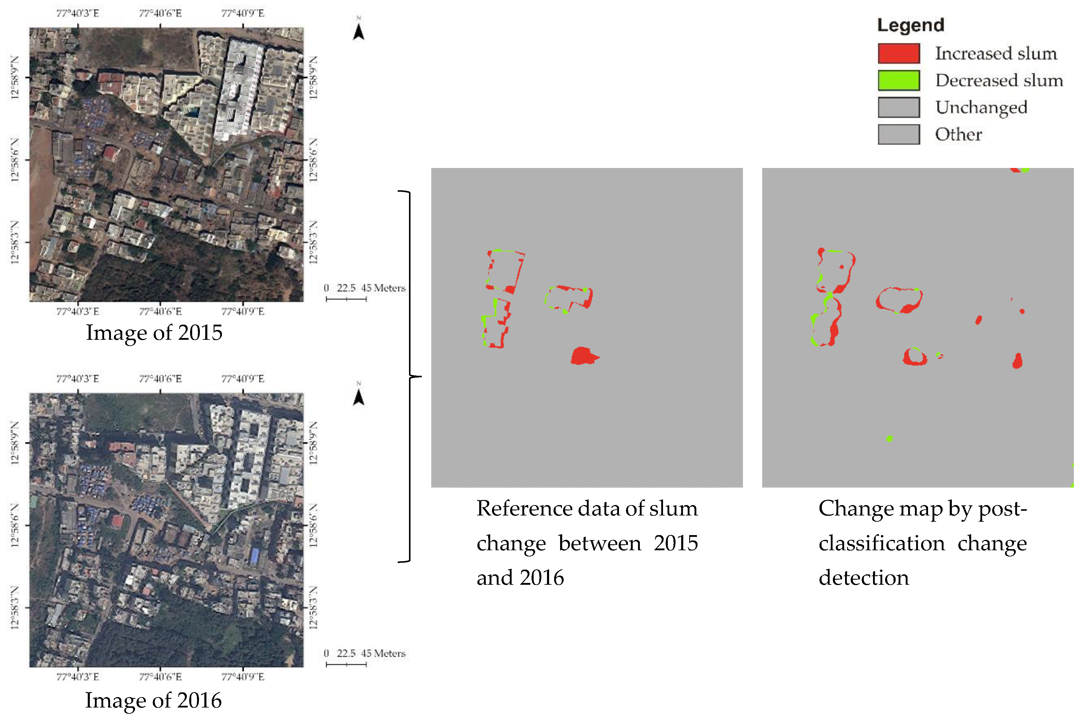
3.2.4. Change Detection Maps
After assessing the accuracy quantitatively, we also visually checked the change maps (see Supplementary Materials). Although the accuracy assessed in the previous section was relatively low for some areas, they often showed the right locations where changes happened. Such an example is shown in Figure 10. The post-classification change-detection result of temporary slums from 2015 to 2016 for this tile had an F1-score of 42.71% based on the confusion matrix. However, the map shows that the general locations and types of changes (increasing/decreasing) were correctly identified. Consequently, the result can be used to determine the slum change location.
4. Discussion
4.1. Temporal Dynamics of Slums in Bangalore
As mentioned before, only a few studies have analyzed the temporal changes of slums. For example, Kit and Lüdeke [8] identified three trends of slum temporal changes: Densification of slum settlements, slum growth in the urban fringe, and the areas which had the most slum growth. The area of changed slums was calculated for the result change maps with a comparison with the reference data (shown in Table 15).
Here, ‘increase’ and ‘decrease’ represent the changes from other classes to temporary slums and from temporary slums to other land uses. The overall gap between reference data and post-classification is 13,579 m2, while for change-detection networks, it is 20,579 m2. Although the change-detection networks show a comparable accuracy in the assessments, they have a higher extensional uncertainty (worse capturing of the area’s extent).
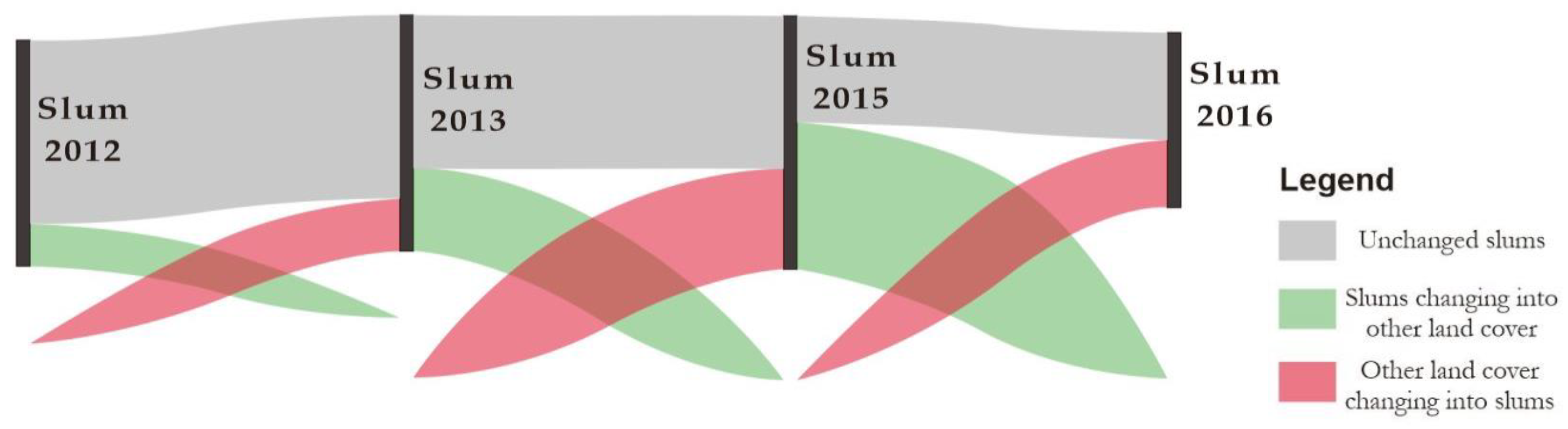
From 2012 to 2016, 12,012 m2 of temporary slums appeared in the study area, while 17,052 m2 disappeared in this time period. There were also 11,041 m2 of unchanged slum area. On average, 7173 m2 of land changed into temporary slums in our study area per year, while 8390 m2 of the temporary slums disappeared, showing an overall decreasing trend. A detailed changing pattern is shown in Figure 11. The flow of the grey color represents how many slums remained unchanged in each time period. The flow of the green color represents the areas changing from slums to other classes, while the red color stands for the areas becoming slums. Thus, with time, fewer slum areas remained unchanged while more and more slum areas were disappearing. The largest increase in temporary slums happened between 2013 to 2015, which was also the longest period in our study period.
4.2. The Pattern of Slum Changing
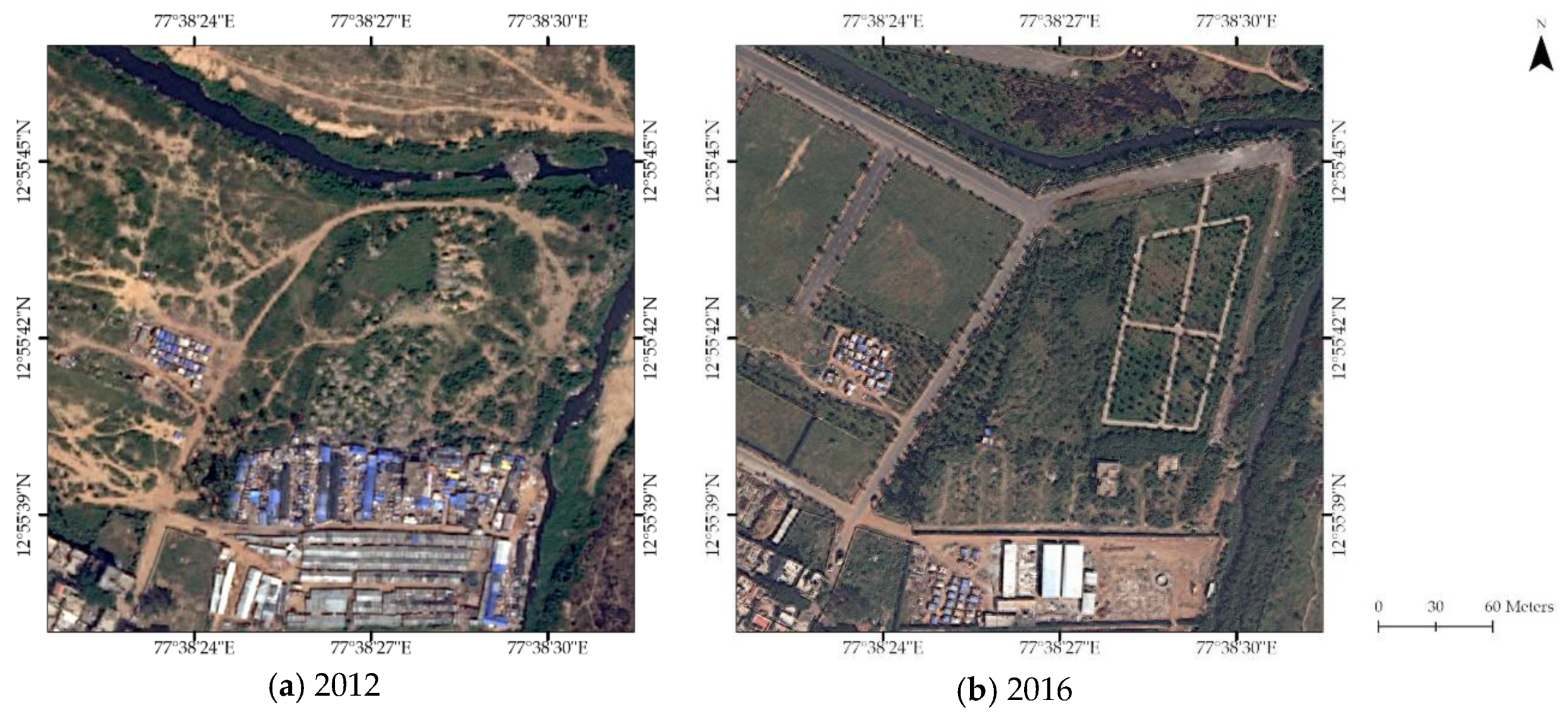
The proportions of different types of temporal dynamics from 2012 to 2016 are shown in Table 16, as well as the rate of change of every temporal dynamic. The largest transition (increase) was the change from vacant land into slums. About 42% of the new slums grew on vacant land, with a change rate of 1447 m2 per year. For the slums’ decreasing, most of the temporary slums changed into green land with a change rate of 2250 m2 per year, which was different from the increasing transition. A very specific example of this transition is shown in Figure 12. This transition was associated with some reforming projects in this area, i.e., formal roads have been constructed in this area, with newly planted green land.
4.3. Methodological Advantages and Disadvantages
In this study, two change detection methods were employed to analyze the temporal dynamics of slums, followed by two methods for accuracy assessment. For post-classification change detection, land-use classification maps were generated based on FCNs. The maps have a high accuracy of over 85%, indicating that using a deep learning algorithm to identify temporary slums from VHR imagery in urban areas is effective. This result also responds to a recent study [26] which showed that FCNs work well to capture informal settlements in Dar es Salaam in Tanzania and Bangalore in India. However, the post-classification change-detection results did not have similar good performances; they did not allow the exact quantification of the change areas. This problem is associated with the uncertainty of slum boundaries, as the reference data were generated by visual interpretation, which tends to be more generalized than the results of image classification, showing extensional uncertainties [42,43]. However, the resulting change maps could identify the existence of changes, i.e., the changed slum areas (location) in the reference maps were also captured by the change-detection results. Molenaar [44] proposed two concepts of existential uncertainty and extensional uncertainty. Existential uncertainty means the uncertainty about the existence of a slum in reality, and extensional uncertainty implies the uncertainty of whether an area covered by a slum can be determined with limited certainty or not [42]. Based on these concepts, the post-classification method is beneficial in analyzing the existence of changes, but not the exact sizes of changed slum areas.
An FCN with the same architecture as the one used for the land-use classification was employed to directly detect the changed slum areas. One of the problems for this method is that the accuracies for the training tiles were much higher than for the testing tiles, indicating that what the classifier learned through the FCNs was not well transferred to the other images. This might also have resulted from the reference data preparation. In addition to the uncertainty of slum delineation, which is the same in the post-classification process, another uncertainty is the change trajectory. In this study, when selecting the training tiles, we only considered the trajectories between temporary slums and our determined land-use classed. In fact, the objects in one land-use class might be different from each other. For example, one training tile contained a trajectory from concrete buildings to temporary slums and taught the networks how to classify it. But in the testing tiles, the trajectory was from brick buildings to temporary slums. Thus, the networks had no knowledge about this specific trajectory, leading to incorrect classification. The change-detection networks had an 87% accuracy for the training tiles, indicating that it has the potential to detect changes when it is well trained. Besides, similar to post-classification, the change-detection networks performed well when identifying the existence of change.
4.4. Accuracy Assessment
In this study, the confusion matrix and trajectory error matrix were employed to assess the accuracy of change detection results. The confusion matrix and related indices, like producer accuracy and user accuracy, are still widely used methods for assessing the accuracy of deep learning algorithms (classification and change detection) [26,28,45]. In this study, the change-detection results did not have high F1-scores; however, the results could detect the correct location of where changes occurred. As the confusion matrix provides a pixel-based result, uncertainties along the boundaries are high and result in low accuracies. Without a standard definition of a slum area and rules on how to draw boundaries, the boundaries of changed areas are fuzzy. Therefore, the confusion matrix cannot give a credible assessment with the consideration of an area (neighborhood) context.
Another assessment method employed in this study was the trajectory error matrix. While the confusion matrix provided an assessment of ‘change/no change’ status, which also addressed the sensitivity and specificity of binary classification [46], TEM assessed the accuracy for ‘from/to’ changes. One shortcoming of the TEM is that random samples are not suitable for analyzing changes, especially when the changed areas only cover a small proportion of the whole region. Therefore, it is recommended for further studies to combine the assessment of change uncertainties with a focus on areas and the change trajectories.
5. Conclusions
An FCN-based approach was developed to map and analyze the temporal dynamics of slums in the city of Bangalore. Temporary slums, also known as “blue tent” slums, generally show a quite high dynamic. Using an FCN architecture with dilated convolutions, we found that a 3 × 3 network had slightly better accuracy (88.38%) compared with that of a 5 × 5 network (86.32%). The results show that 17,052 m2 of slum areas disappeared and 12,012 m2 of new slums developed between 2016 and 2012, showing an overall decrease in slum areas. However, when analyzing the change trajectories, it was surprising that slums were generally not transformed or upgraded, but were more often changed into green areas while new slums developed on vacant land. This has implications for urban planning and management, as slums do not exist for long periods at the same spot; still, dwellers would require basic services, which need to be much more flexible and tailored to the high spatio-temporal dynamics of such areas. Furthermore, we know very little about the living conditions in these areas as they are not (well) covered in official statistics (e.g., census), and socio-economic surveys will commonly omit such small pockets, as they are not easily included in sampling frameworks without spatial data on them. Therefore, spatial data, even of moderate accuracies, on these highly dynamic slums are essential for addressing a totally overlooked dimension of urban deprivation, namely the one of temporary settlements, which can be found across Indian cities and in many other rapidly developing cities of the global South.
Supplementary Materials
The following are available online at https://www.mdpi.com/2072-4292/11/23/2844/s1.
Author Contributions
M.K., C.P., and R.L. developed the structure of the research. R.L. performed the analysis and wrote the majority of the paper, under the supervision and revision of M.K. and C.P.
Funding
This research received no external funding.
Acknowledgments
The authors greatly appreciate the support provided by the project Dynaslum (Data Driven Modelling and Decision Support for Slums) project (contract number:27015G05), which are managed by the Dutch national research council (NWO), for providing the data for this research.
Conflicts of Interest
The authors declare no conflict of interest.
References
- United Nations. UN-DESA World Urbanization Prospects: The 2018 Revision; United Nations: New York, NY, USA, 2018. [Google Scholar]
- Kohli, D.; Sliuzas, R.; Kerle, N.; Stein, A. An ontology of slums for image-based classification. Comput. Environ. Urban Syst. 2012, 36, 154–163. [Google Scholar] [CrossRef]
- UN-HABITAT. State of the World’s Cities, 2006/2007: 30 Years of Shaping the Habitat Agenda; UN-HABITAT: London, UK, 2006. [Google Scholar]
- UN General Assembly. Transforming Our World: The 2030 Agenda for Sustainable Development; United Nations: New York, NY, USA, 2015. [Google Scholar]
- Mahabir, R.; Crooks, A.; Croitoru, A.; Agouris, P.; Mahabir, R.; Crooks, A.; Croitoru, A.; The, P.A. The study of slums as social and physical constructs: Challenges and emerging research opportunities. Reg. Stud. Reg. Sci. 2016, 3, 400–420. [Google Scholar] [CrossRef]
- Kuffer, M.; Pfeffer, K.; Sliuzas, R. Slums from space-15 years of slum mapping using remote sensing. Remote Sens. 2016, 8, 455. [Google Scholar] [CrossRef]
- Ranguelova, E.; Weel, B.; Roy, D.; Kuffer, M.; Pfeffer, K.; Lees, M. Image based classification of slums, built-up and non-built-up areas in Kalyan and Bangalore, India. Eur. J. Remote Sens. 2019, 52 (Suppl. S1), 40–61. [Google Scholar] [CrossRef]
- Kit, O.; Lüdeke, M. Automated detection of slum area change in Hyderabad, India using multitemporal satellite imagery. ISPRS J. Photogramm. Remote Sens. 2013, 83, 130–137. [Google Scholar] [CrossRef]
- Veljanovski, T.; Kanjir, U.; Pehani, P.; Otir, K.; Kovai, P. Object-Based Image Analysis of VHR Satellite Imagery for Population Estimation in Informal Settlement Kibera-Nairobi, Kenya. In Remote Sensing—Applications; Escalante, B., Ed.; InTech: Rijeka, Croatia, 2012; pp. 407–434. ISBN 978-953-51-0651-7. [Google Scholar]
- Pratomo, J.; Kuffer, M.; Kohli, D.; Martinez, J. Application of the trajectory error matrix for assessing the temporal transferability of OBIA for slum detection. Eur. J. Remote Sens. 2018, 51, 838–849. [Google Scholar] [CrossRef]
- Kohli, D.; Warwadekar, P.; Kerle, N.; Sliuzas, R.; Stein, A. Transferability of object-oriented image analysis methods for slum identification. Remote Sens. 2013, 5, 4209–4228. [Google Scholar] [CrossRef]
- Kuffer, M.; Pfeffer, K.; Sliuzas, R.; Baud, I. Extraction of Slum Areas From VHR Imagery Using GLCM Variance. IEEE J. Sel. Top. Appl. Earth Obs. Remote Sens. 2016, 9, 1830–1840. [Google Scholar] [CrossRef]
- Hofmann, P.; Strobl, J.; Blaschke, T.; Kux, H. Detecting informal settlements from QuickBird data in Rio de Janeiro using an object based approach. In Object-Based Image Analysis; Springer: Berlin/Heidelberg, Germany, 2008; pp. 531–553. ISBN 3540770577. [Google Scholar]
- Badmos, O.S.; Rienow, A.; Callo-Concha, D.; Greve, K.; Jürgens, C. Simulating slum growth in Lagos: An integration of rule based and empirical based model. Comput. Environ. Urban Syst. 2019, 77, 101369. [Google Scholar] [CrossRef]
- Bachofer, F.; Murray, S. Remote Sensing for Measuring Housing Supply in Kigali Remote Sensing for Measuring Housing Supply in Kigali, Final Report CONTENT; International Growth Centre: London, UK, 2018. [Google Scholar]
- Liu, H.; Huang, X.; Wen, D.; Li, J. The use of landscape metrics and transfer learning to explore urban villages in China. Remote Sens. 2017, 9, 365. [Google Scholar] [CrossRef]
- Duque, J.C.; Patino, J.E.; Betancourt, A. Exploring the potential of machine learning for automatic slum identification from VHR imagery. Remote Sens. 2017, 9, 895. [Google Scholar] [CrossRef]
- Verma, D.; Jana, A.; Ramamritham, K. Transfer learning approach to map urban slums using high and medium resolution satellite imagery. Habitat Int. 2019, 88, 101981. [Google Scholar] [CrossRef]
- Wang, J.; Kuffer, M.; Roy, D.; Pfeffer, K. Deprivation pockets through the lens of convolutional neural networks. Remote Sens. Environ. 2019, 234, 111448. [Google Scholar] [CrossRef]
- Wurm, M.; Stark, T.; Zhu, X.X.; Weigand, M.; Taubenböck, H. Semantic segmentation of slums in satellite images using transfer learning on fully convolutional neural networks. ISPRS J. Photogramm. Remote Sens. 2019, 150, 59–69. [Google Scholar] [CrossRef]
- Ma, L.; Liu, Y.; Zhang, X.; Ye, Y.; Yin, G.; Johnson, B.A. Deep learning in remote sensing applications: A meta-analysis and review. ISPRS J. Photogramm. Remote Sens. 2019, 152, 166–177. [Google Scholar] [CrossRef]
- Bergado, J.R.; Persello, C.; Stein, A. Recurrent Multiresolution Convolutional Networks for VHR Image Classification. IEEE Trans. Geosci. Remote Sens. 2018, 56, 6361–6374. [Google Scholar] [CrossRef]
- Paisitkriangkrai, S.; Sherrah, J.; Janney, P.; Van Den Hengel, A. Semantic Labeling of Aerial and Satellite Imagery. IEEE J. Sel. Top. Appl. Earth Obs. Remote Sens. 2016, 9, 2868–2881. [Google Scholar] [CrossRef]
- Mboga, N.; Persello, C.; Bergado, J.R.; Stein, A. Detection of informal settlements from VHR images using convolutional neural networks. Remote Sens. 2017, 9, 1106. [Google Scholar] [CrossRef]
- Ajami, A.; Kuffer, M.; Persello, C.; Pfeffer, K. Identifying a Slums’ Degree of Deprivation from VHR Images Using Convolutional Neural Networks. Remote Sens. 2019, 11, 1282. [Google Scholar] [CrossRef]
- Persello, C.; Stein, A. Deep Fully Convolutional Networks for the Detection of Informal Settlements in VHR Images. IEEE Geosci. Remote Sens. Lett. 2017, 14, 2325–2329. [Google Scholar] [CrossRef]
- Sun, W.; Wang, R. Fully Convolutional Networks for Semantic Segmentation of Very High Resolution Remotely Sensed Images Combined with DSM. IEEE Geosci. Remote Sens. Lett. 2018, 15, 474–478. [Google Scholar] [CrossRef]
- Fu, G.; Liu, C.; Zhou, R.; Sun, T.; Zhang, Q. Classification for high resolution remote sensing imagery using a fully convolutional network. Remote Sens. 2017, 9, 498. [Google Scholar] [CrossRef]
- Zhu, X.X.; Tuia, D.; Mou, L.; Xia, G.-S.; Zhang, L.; Xu, F.; Fraundorfer, F. Deep learning in remote sensing: A comprehensive review and list of resources. IEEE Geosci. Remote Sens. Mag. 2017, 5, 8–36. [Google Scholar] [CrossRef]
- Government of India Census 2011 India. Available online: http://www.census2011.co.in/ (accessed on 23 August 2018).
- Census Organization of India Bangalore (Bengaluru) City Population Census 2011–2019|Karnataka. Available online: https://www.census2011.co.in/census/city/448-bangalore.html (accessed on 14 February 2019).
- Roy, D.; Lees, M.H.; Pfeffer, K.; Sloot, P.M.A. Spatial segregation, inequality, and opportunity bias in the slums of Bengaluru. Cities 2018, 74, 269–276. [Google Scholar] [CrossRef]
- Government of India. Slums in India: A Statistical Compendium 2015; Ministry of Housing and Urban Poverty Alleviation, National Buildings Organization: New Delhi, India, 2015.
- Krishna, A.; Sriram, M.S.; Prakash, P. Slum types and adaptation strategies: Identifying policy-relevant differences in Bangalore. Environ. Urban. 2014, 26, 568–585. [Google Scholar] [CrossRef]
- DynaSlum. Available online: http://www.dynaslum.com/ (accessed on 23 August 2018).
- Bergado, J.R.; Persello, C.; Gevaert, C. A deep learning approach to the classification of sub-decimetre resolution aerial images. In Proceedings of the International Geoscience and Remote Sensing Symposium (IGARSS), Beijing, China, 10–15 July 2016; Volume 2016-Novem, pp. 1516–1519. [Google Scholar]
- Yu, F.; Koltun, V. Multi-Scale Context Aggregation by Dilated Convolutions. arXiv 2015, arXiv:1511.07122. [Google Scholar]
- Maas, A.L.; Hannun, A.Y.; Ng, A.Y. Rectifier nonlinearities improve neural network acoustic models. In Proceedings of the International Conference on Machine Learning (ICML), Atlanta, GA, USA, 16–21 June 2013; Volume 30, p. 3. [Google Scholar]
- Szegedy, C.; Vanhoucke, V.; Ioffe, S.; Shlens, J.; Wojna, Z. Rethinking the Inception Architecture for Computer Vision. In Proceedings of the IEEE Conference on Computer Vision and Pattern Recognition, Las Vegas, NV, USA, 26 June–1 July 2016; pp. 2818–2826. [Google Scholar]
- Radoux, J.; Bogaert, P. Good practices for object-based accuracy assessment. Remote Sens. 2017, 9, 646. [Google Scholar] [CrossRef]
- Li, B.; Zhou, Q. Accuracy assessment on multi-temporal land-cover change detection using a trajectory error matrix. Int. J. Remote Sens. 2009, 30, 1283–1296. [Google Scholar] [CrossRef]
- Kohli, D.; Stein, A.; Sliuzas, R. Uncertainty analysis for image interpretations of urban slums. Comput. Environ. Urban Syst. 2016, 60, 37–49. [Google Scholar] [CrossRef]
- Kuffer, M.; Wang, J.; Nagenborg, M.; Pfeffer, K.; Kohli, D.; Sliuzas, R.; Persello, C. The Scope of Earth-Observation to Improve the Consistency of the SDG Slum Indicator. ISPRS Int. J. Geo Inf. 2018, 7, 428. [Google Scholar] [CrossRef]
- Molenaar, M. Three conceptual uncertainty levels for spatial objects. Int. Arch. Photogramm. Remote Sens. 2000, 33, 670–677. [Google Scholar]
- Dai, F.; Wang, Q.; Gong, Y.; Chen, G.; Zhang, X.; Zhu, K. Change detection based on Faster R-CNN for high-resolution remote sensing images. Remote Sens. Lett. 2018, 9, 923–932. [Google Scholar]
- Foody, G.M. Assessing the accuracy of land cover change with imperfect ground reference data. Remote Sens. Environ. 2010, 114, 2271–2285. [Google Scholar] [CrossRef] [Green Version]
Figure 1.
Example of shelters of blue plastic sheeting and small unit size [34].
Figure 1.
Example of shelters of blue plastic sheeting and small unit size [34].

Figure 2.
Example of one rapidly changing slum area (Source: Google Earth).

Figure 3.
Distribution of study tiles (tiles shown in red) in the WorldView image (06.01.2016) (Source: DigitalGlobe).
Figure 3.
Distribution of study tiles (tiles shown in red) in the WorldView image (06.01.2016) (Source: DigitalGlobe).

Figure 4.
The workflow of the two change detection approaches.

Figure 5.
Kernels with an increasing receptive field: (a) a receptive field of 3 × 3 with a dilation factor of one; (b) a receptive field of 7 × 7 with a dilation factor of two; (c) a receptive field of 15 × 15 with a dilation factor of three.
Figure 5.
Kernels with an increasing receptive field: (a) a receptive field of 3 × 3 with a dilation factor of one; (b) a receptive field of 7 × 7 with a dilation factor of two; (c) a receptive field of 15 × 15 with a dilation factor of three.

Figure 6.
Example architecture: (a) Two 3 × 3 convolutions and (b) replacing one 5 × 5.

Figure 7.
Classification map example and its image of 2016, showing patches of pixel islands within the red boxes (reclassifying the Green land, Vacant land, Formally built-up, and Other from original results to one class of Non-slum in order to better illustrate the pixel island problem).
Figure 7.
Classification map example and its image of 2016, showing patches of pixel islands within the red boxes (reclassifying the Green land, Vacant land, Formally built-up, and Other from original results to one class of Non-slum in order to better illustrate the pixel island problem).

Figure 8.
Comparison of the original classification and noise reduction results.

Figure 9.
Example of stacked maps for change-detection accuracy assessment.

Figure 10.
Example with a low accuracy but the correct location of change.

Figure 11.
Diagram of the change in temporary slums.

Figure 12.
Example of slums changing into green land.


Table 1.
Summary of the image dataset used in this study.
| Satellite | Resolution | Band Number | Time |
|---|---|---|---|
| WorldView 2 | 0.5 × 0.5 m (multispectral) | 8 bands | 01.12.2012 |
| 2.0 × 2.0 m (panchromatic) | 24.04.2013 | ||
| WorldView 3 | 0.3 × 0.3 m (multispectral) | 8 bands | 16.02.2015 |
| 1.2 × 1.2 m (panchromatic) | 06.01.2016 |
Table 2.
Land-use classes for the reference data.
| Class | Description | Label | Count |
|---|---|---|---|
| Temporary slum | Tents with blue plastic sheeting and small unit size | 1 | 1,328,901 |
| Green land | Open land covered by vegetation | 2 | 4,843,864 |
| Vacant land | Bare soil land | 3 | 3,687,606 |
| Formally built-up | Formal buildings, roads | 4 | 10,984,295 |
| Other | Car park, water body, etc. | 5 | 488,007 |
Table 3.
Reference data classes for the change-detection net.
| Class | Description | Land-Use in T1 | Land-Use in T2 | Label |
|---|---|---|---|---|
| Increased slum | Temporary slum did not exist in T1 but appeared in T2. | Green land Vacant land Formally built-up Other | Temporary slum | 1 |
| Decreased slum | Temporary slum existed in T1 but disappeared in T2. | Temporary slum | Green land Vacant land Formally built-up Other | 2 |
| Unchanged slum | Temporary slum stayed unchanged between T1 and T2 | Temporary slum | Temporary slum | 3 |
| Other | Other land use | Green land Vacant land Formally built-up Other | Green land Vacant land Formally built-up Other | 4 |
| T1: An earlier year | T2: A later year |
Table 4.
Structure of the 5 × 5 FCNs architecture.
| Layer | Module Type | Dimension | Dilation | Stride | Pad |
|---|---|---|---|---|---|
| DK1 | convolution | 5 × 5 × 8 × 16 | 1 | 1 | 2 |
| lReLUs | |||||
| DK2 | convolution | 5 × 5 × 16 × 32 | 2 | 1 | 4 |
| lReLUs | |||||
| DK3 | convolution | 5 × 5 × 32 × 32 | 3 | 1 | 6 |
| lReLUs | |||||
| DK4 | convolution | 5 × 5 × 32 × 32 | 4 | 1 | 8 |
| lReLUs | |||||
| DK5 | convolution | 5 × 5 × 32 × 32 | 5 | 1 | 10 |
| lReLUs | |||||
| DK6 | convolution | 5 × 5 × 32 × 32 | 6 | 1 | 12 |
| lReLUs | |||||
| Class. | convolution | 1 × 1 × 32 × 5 | 1 | 1 | 0 |
| softmax |
Table 5.
Structure of the 3 × 3 FCNs architecture.
| Layer | Module Type | Dimension | Dilation | Stride | Pad |
|---|---|---|---|---|---|
| DK1 | convolution | 3 × 3 × 8 × 16 | 1 | 1 | 1 |
| lReLUs | |||||
| convolution | 3 × 3 × 16 × 16 | 1 | 1 | 1 | |
| lReLUs | |||||
| DK2 | convolution | 3 × 3 × 16 × 32 | 2 | 1 | 2 |
| lReLUs | |||||
| convolution | 3 × 3 × 32 × 32 | 2 | 1 | 2 | |
| lReLUs | |||||
| DK3 | convolution | 3 × 3 × 32 × 32 | 3 | 1 | 3 |
| lReLUs | |||||
| convolution | 3 × 3 × 32 × 32 | 3 | 1 | 3 | |
| lReLUs | |||||
| DK4 | convolution | 3 × 3 × 32 × 32 | 4 | 1 | 4 |
| lReLUs | |||||
| convolution | 3 × 3 × 32 × 32 | 4 | 1 | 4 | |
| lReLUs | |||||
| DK5 | convolution | 3 × 3 × 32 × 32 | 5 | 1 | 5 |
| lReLUs | |||||
| convolution | 3 × 3 × 32 × 32 | 5 | 1 | 5 | |
| lReLUs | |||||
| DK6 | convolution | 3 × 3 × 32 × 32 | 6 | 1 | 6 |
| lReLUs | |||||
| convolution | 3 × 3 × 32 × 32 | 6 | 1 | 6 | |
| lReLUs | |||||
| Class. | convolution | 1 × 1 × 32 × 5 | 1 | 1 | 0 |
| softmax |
Table 6.
Land-use class label of classification map after reclassifying.
| Year | Land-Use Class Label | ||||
|---|---|---|---|---|---|
| Temporary Slum | Green Land | Vacant Land | Formal Built-Up | Other | |
| 2012 | 1 | 2 | 3 | 4 | 5 |
| 2013 | 10 | 20 | 30 | 40 | 50 |
| 2015 | 100 | 200 | 300 | 400 | 500 |
| 2016 | 1000 | 2000 | 3000 | 4000 | 5000 |
Table 7.
Sub-groups in the trajectory error matrix (TEM).
| Groups | Classification Situation | Interpretations |
|---|---|---|
| S1 | Correct | Correctly detected as non-changed with the correct classification |
| S2 | Correctly detected as a changed slum with correct trajectory | |
| S3 | Incorrect | Correctly detected as non-changed with an incorrect classification |
| S4 | Incorrectly detected as changed slum | |
| S5 | Incorrectly detected as non-changed | |
| S6 | Correctly detected as a changed slum with an incorrect trajectory |
Table 8.
Accuracies (precision, recall, F1 score) of two networks mapping temporary slums.
| 5 × 5 Networks | 3 × 3 Networks | |||||
|---|---|---|---|---|---|---|
| Precision | Recall | F1-Score | Precision | Recall | F1-Score | |
| 2012 | 85.57% | 97.04% | 90.85% | 85.79% | 96.99% | 90.95% |
| 2013 | 84.20% | 97.00% | 90.03% | 84.32% | 96.02% | 89.55% |
| 2015 | 81.55% | 85.76% | 83.29% | 84.41% | 89.69% | 86.82% |
| 2016 | 74.40% | 85.76% | 81.97% | 79.44% | 89.69% | 86.58% |
| In total | 81.10% | 93.19% | 86.32% | 83.30% | 96.55% | 88.38% |
Table 9.
F1-scores showing the accuracies after noise reduction (based on the 3 × 3 network results).
Table 9.
F1-scores showing the accuracies after noise reduction (based on the 3 × 3 network results).
| Original Classification | Majority Analysis | Classification Clumping | |
|---|---|---|---|
| 2012 | 90.95% | 89.38% | 87.39% |
| 2013 | 89.55% | 89.19% | 86.43% |
| 2015 | 86.82% | 88.03% | 86.21% |
| 2016 | 86.58% | 86.80% | 84.23% |
| In total | 88.38% | 88.35% | 86.06% |
Table 10.
Accuracies (precision, recall, F1 score) of two networks for change detection net.
| 5 × 5 Networks | 3 × 3 Networks | |||||
|---|---|---|---|---|---|---|
| Precision | Recall | F1-Score | Precision | Recall | F1-Score | |
| 2012–2013 | 13.85% | 42.26% | 20.25% | 12.75% | 40.42% | 18.31% |
| 2013–2015 | 34.79% | 42.31% | 36.01% | 31.87% | 52.59% | 37.88% |
| 2015–2016 | 22.41% | 47.46% | 28.76% | 31.52% | 54.17% | 36.49% |
| In total | 23.68% | 44.01% | 28.34% | 25.38% | 49.06% | 30.89% |
Table 11.
F1-scores of changed slum area in the post-classification results.
| Post-Classification | Change-Detection Networks | |
|---|---|---|
| 2012–2013 | 43.69% | 49.69% |
| 2013–2015 | 61.52% | 60.66% |
| 2015–2016 | 55.95% | 50.96% |
| In total | 53.80% | 53.68% |
Table 12.
F1-scores of change-detection results for each tile (the training tiles shown in red color).
Table 12.
F1-scores of change-detection results for each tile (the training tiles shown in red color).
| Tile | Post-Classification | Change-Detection Networks | ||||
|---|---|---|---|---|---|---|
| 2012–2013 | 2013–2015 | 2015–2016 | 2012–2013 | 2013–2015 | 2015–2016 | |
| 1 | 36.67% | 38.42% | 11.92% | 22.69% | 19.89% | 3.86% |
| 2 | 37.19% | 55.15% | 55.00% | 19.31% | 51.32% | 40.37% |
| 3 | 41.66% | 70.22% | 51.31% | 78.46% | 89.30% | 73.27% |
| 4 | 28.87% | 63.24% | 42.71% | 17.79% | 54.50% | 24.37% |
| 5 | 54.70% | 73.69% | 70.20% | 91.54% | 94.97% | 91.29% |
| 6 | 36.13% | 57.11% | 47.94% | 23.66% | 36.65% | 39.20% |
| 7 | 62.28% | 82.82% | 92.63% | 91.29% | 95.20% | 96.93% |
| 8 | * | * | 73.58% | * | * | 48.65% |
| 9 | 62.58% | 72.98% | 63.93% | 84.70% | 86.48% | 75.51% |
| 10 | 33.11% | 40.03% | 50.31% | 17.78% | 17.68% | 16.12% |
| Tile 3/5/7/9: Training tiles * No changes in this tile | ||||||
Table 13.
F1-scores of the training and testing tiles.
| Tile | Method | 2012–2013 | 2013–2015 | 2015–2016 | In Total |
|---|---|---|---|---|---|
| Training | Post-classification | 55.30% | 74.93% | 69.52% | 66.58% |
| Change-detection networks | 86.50% | 91.49% | 84.25% | 87.41% | |
| Testing | Post-classification | 34.39% | 50.79% | 46.91% | 44.21% |
| Change-detection networks | 20.25% | 36.01% | 28.76% | 28.37% |
Table 14.
TEM indices for two change detection methods.
| Indices | Post-Classification | Change-Detection Networks |
|---|---|---|
| overall accuracy (AT) | 76.36% | 72.30% |
| change/no change accuracy (AC/N), | 89.60% | 80.12% |
| overall accuracy difference (OAD) | 13.24% | 7.82% |
| accuracy difference of no change trajectory (ADICN) | 100.00% | 100.00% |
| accuracy difference of change trajectory (ADICC) | 67.18% | 74.17% |
Table 15.
Area of changed slums in different time intervals.
| 2012–2013 | 2013–2015 | 2015–2016 | ||||
|---|---|---|---|---|---|---|
| (m2) | Increase | Decrease | Increase | Decrease | Increase | Decrease |
| Reference data | 8873 | 4047 | 12,614 | 9652 | 7203 | 19,860 |
| Post-classification | 7981 | 6377 | 15,205 | 12,471 | 10,030 | 21,980 |
| Change-detection networks | 4826 | 2612 | 9313 | 13,403 | 5654 | 13,364 |
Table 16.
Proportion and changing rate of different temporal dynamics, 2012 to 2016.
| Increased | Decreased | ||||
|---|---|---|---|---|---|
| Proportion | Changing Rate (m2/Year) | Proportion | Changing Rate (m2/Year) | ||
| other → slum | 0.64% | 22 | slum → green land | 42.64% | 2250 |
| formally built-up → slum | 24.11% | 819 | slum → vacant land | 36.71% | 1937 |
| green land → slum | 32.68% | 1111 | slum → formally built-up | 20.51% | 1083 |
| vacant land → slum | 42.57% | 1447 | slum → other | 0.14% | 7 |
© 2019 by the authors. Licensee MDPI, Basel, Switzerland. This article is an open access article distributed under the terms and conditions of the Creative Commons Attribution (CC BY) license (http://creativecommons.org/licenses/by/4.0/).
Share and Cite
MDPI and ACS Style
Liu, R.; Kuffer, M.; Persello, C. The Temporal Dynamics of Slums Employing a CNN-Based Change Detection Approach. Remote Sens. 2019, 11, 2844. https://doi.org/10.3390/rs11232844
AMA Style
Liu R, Kuffer M, Persello C. The Temporal Dynamics of Slums Employing a CNN-Based Change Detection Approach. Remote Sensing. 2019; 11(23):2844. https://doi.org/10.3390/rs11232844
Chicago/Turabian StyleLiu, Ruoyun, Monika Kuffer, and Claudio Persello. 2019. "The Temporal Dynamics of Slums Employing a CNN-Based Change Detection Approach" Remote Sensing 11, no. 23: 2844. https://doi.org/10.3390/rs11232844
Note that from the first issue of 2016, this journal uses article numbers instead of page numbers. See further details here.