Thermohaline Structures and Heat/Freshwater Transports of Mesoscale Eddies in the Bay of Bengal Observed by Argo and Satellite Data

1
Third Institute of Oceanography, Ministry of Natural Resources, Xiamen 361005, China
2
Laboratory for Regional Oceanography and Numerical Modeling, Qingdao National Laboratory for Marine Science and Technology, Qingdao 266237, China
3
Southern Marine Science and Engineering Guangdong Laboratory (Zhuhai), Zhuhai 519082, China
4
Department of Atmospheric and Oceanic Sciences, University of Colorado Boulder, Boulder, CO 80302, USA
*
Author to whom correspondence should be addressed.
Remote Sens. 2019, 11(24), 2989; https://doi.org/10.3390/rs11242989
Submission received: 11 November 2019
/
Revised: 7 December 2019
/
Accepted: 10 December 2019
/
Published: 12 December 2019
(This article belongs to the Section Ocean Remote Sensing)
Abstract
:Knowledge of mesoscale eddies in the Bay of Bengal (BOB) is key for further understanding the climate variability in this region and beyond, but little is known about the vertical structure of these eddies. In this study, the three−dimensional structure and transport characteristics of mesoscale eddies in the BOB were comprehensively investigated by the combined use of Argo profiles and satellite data. The composite analysis showed that eddy−induced ocean anomalies are mainly confined to the upper 300 m of the water. The spatial structure of eddy−induced thermohaline perturbations is characterized by a dominant dipole structure in the near surface layer, arising from horizontal advection of the background thermohaline gradient by eddy rotation, and a monopole structure in the subsurface layer, caused by eddy−induced vertical displacements of the isopycnal surfaces. In the eddy core, the maximum temperature anomalies induced by a cyclonic eddy (CE) and an anticyclonic eddy (AE) are about −1.2 °C and +1.2 °C, respectively. The anomalies are located at approximately 100 m. The corresponding salinity anomalies are located at approximately 50 m with a value of −0.1 psu (0.1 psu) for CE (AE). The eddy thermohaline structure has a seasonal character. A deeper temperature and salinity core occurs in both CE and AE in spring compared to that in other seasons, which is primarily caused by the relatively deep thermocline and halocline during that season. In addition, unique warming anomalies induced by CE are present in the mixed layer during winter due to the vertical advection of the BL (Barrier Layer) warmer water by eddies. The total meridional heat transport induced by the composite eddy is poleward (equatorward) south (north) to 10°N with a value of 0.01 PW (−0.013 PW), whereas the total meridional freshwater transport is equatorward with a value of 0.046 Sv over a one−year period. The volume of freshwater export out of the bay is approximately 35% of the annual net freshwater input from local precipitation and river discharge.

1. Introduction
The Bay of Bengal (BOB), which is located in the northeastern Indian Ocean, is a semi−enclosed marginal sea. Due to the combined influences of the seasonally reversing South Asia monsoon, equatorial remote forcing, and large amounts of freshwater influx from monsoonal rainfall and river discharges (e.g., [1] and references therein), the upper−layer circulation of the BOB is subject to remarkable seasonal variability. The basin−scale surface circulation consists of a strong anticyclonic (cyclonic) gyre during the pre−summer (post−summer) monsoon [2,3], while it becomes very complicated with a multi−gyred pattern for the two monsoon seasons (Figure 1) [1,4]. The western boundary current of the bay (also named the East Indian Coastal Current, i.e., EICC) is sensitive to the variability of basin−scale circulation. Associated with seasonal changes in cyclonic and anticyclonic gyres, the EICC reverses direction twice a year, flowing northeastward from February to September, with a peak in March to April, then flowing southwestward in the remaining months, with the strongest flow occurring in November [5].
For intraseasonal variation, the oceanic circulation in the BOB is characterized by energetic mesoscale−eddy structures. Some common physical properties of mesoscale eddies have been described in previous studies by analyses of individual eddies based on in situ hydrographic measurements (e.g., [3,6,7,8,9,10]). Field observations have shown that eddies are mostly confined to the upper 300 m of the water column (e.g., [8,11]) and have horizontal dimensions of 200 km to 300 km. Most of these observed eddies are located around the EICC [3,8,12,13]. The plausible mechanisms that cause the high occurrence of eddies around the western boundary of the bay include the monsoon conversion, the baroclinic and barotropic instabilities of the EICC, and the energy transmission of the westward Rossby waves [4].
Benefitting from approximately three decades of high spatiotemporal coverage of satellite measurements, the horizontal evolution patterns (e.g., the genesis, polarity, propagation, lifetime and spatiotemporal variability) and kinematic properties of the BOB eddies have been thoroughly investigated through a statistical analysis of altimeter data (e.g., [14,15,16]). The abovementioned eddy−rich domain in the western boundary that was revealed by field observations has been fully confirmed [14,16]. In addition, another critical region for eddy generation is located at the eastern boundary over the BOB, according to altimeter measurements [14,16,17]. The equatorial wind forcing and the instability triggered by the Myanmar bump are the two major reasons for eddy formation in that area [17].
However, until now, very little was known about the vertical structure of eddies in the BOB. Studies aimed at understanding the vertical structure of the BOB eddies have been mainly based on individual shipboard observations (e.g., [4,8,9]), which are often too sparse and restricted over space and time to uncover three−dimensional images of eddies. As such, it has been a challenge to fully capture through field observations the evolving oceanic eddies in terms of their detailed three−dimensional structures. To overcome this challenge, composite analyses of satellite altimeters and Argo data were recently used to reconstruct the mean structures of eddies in various regions of the global oceans (e.g., [18,19,20,21,22,23,24]). Some recent studies [25,26] explored the eddies’ properties through unmanned marine vehicles and high−resolution CTD. Although a similar analysis was carried out in the western bay [27], only the vertical profiles (one−dimension) of the mean anomalies in temperature, salinity, and dynamic height inside eddies were depicted in the study, which suggests that both anticyclonic and cyclonic eddies have a single core vertical structure, with the core located at a depth of approximately 100 dbar. In another recent study [17], a truly three−dimensional thermal structure of a composite anticyclonic/cyclonic eddy over the central bay was presented for the first time and revealed the subsurface intensification of eddies. To date, a full image of the three−dimensional structures of temperature, salinity, and velocity inside eddies is still absent in the BOB. As is well−known, the upper−layer temperature and salinity in the BOB have distinct seasonal variations [1,28]. In particular, a very sharp salinity stratification accommodating a temperature−inversion layer with warmer temperatures than those at the surface layer has been reported to frequently occur in conjunction with barrier layers during winter [29]. Under the strong unique annual cycle of hydrographic background, the seasonality for eddy vertical structure is also not yet clear. Therefore, one of the purposes of this study was to combine satellite−detected eddy signals with temperature/salinity data profiles from Argo floats to construct three−dimensional images of eddies and to examine their seasonal variations.
In addition, as eddies are one of the most energetic flows in the ocean, they contribute important horizontal heat and salt transports on both regional and global scale (e.g., [22,30,31,32]), which are critical in maintaining regional and global climate states. However, due to insufficiency of data, an observation−based three−dimensional picture of eddy−induced heat and salt transport has not yet been quantitatively specified in the BOB, and was thus explored in the present study.
The rest of the paper is organized as follows. The data and methods used in this study are described in Section 2. The mean and variability of sea surface salinity (SSS) and sea surface temperature (SST), together with the mean eddy statistical characteristics, are presented in Section 3, which is followed by the mean reconstructed eddy structure and meridional flux (Section 4). Seasonal variations of eddy structure, eddy−induced meridional heat, and freshwater transport are then discussed in Section 5. Finally, the main findings of this paper are summarized in Section 6.
2. Data and Methods
2.1. Data
The daily Mesoscale Eddy Trajectory Atlas (META) dataset [33] produced by Collecte Localization Satellites (CLS) and made available through Archiving, Validation, and Interpretation of Satellite Oceanographic Data+ (AVISO+) for the period of 7 November 2001 to 25 September 2016 was used to examine spatial patterns of eddies and to localize eddies to reconstruct their structure using Argo profiles. The dataset was composed of the coordinates of the eddy centers and the amplitudes, radii, and rotational velocities for eddies identified and tracked from their surface signature in daily sea level anomaly (SLA) fields [33]. The detection method used on the META dataset was first developed by Chelton et al. [34], and it has been extensively applied for mesoscale eddies automatically detected from satellite altimetry data. In this method, eddy centers are first identified by searching for the local SLA minima/maxima from the two−sat−merged SLA maps after application of a spatial high−pass filter and are then detected and tracked by the algorithms based on the Okubo−Weiss parameter [34]. Only those eddies with an amplitude larger than 1 cm and a lifetime longer than four weeks were documented in the META dataset.
Argo profiles provided by the Institute Français de Recherche Pour l’Exploitation de la Mer (IFREMER, data are available at ftp://ftp.ifremer.fr/ifremer/argo/) for 7 November 2001 to 25 September 2016, the same period as that of the META dataset, were used to reconstruct the three−dimensional structure of eddies. Although these profiles have undergone automatic preprocessing and quality control procedures by the Argo data center [35], some additional quality controls were applied in this study. The profiles whose positions and times were not flagged as good were discarded, and among the remaining profiles, only the individual records flagged as good were retained. Similar to those in the studies of Chaigneau et al. [19] and Yang et al. [21], the selected profiles needed to satisfy the following standards: Each profile should have at least 30 vertical measurements above 500 m, and the depth difference between two consecutive measurements in the depth range 0–100 m, 100–300 m, and deeper than 300 m must not exceed 25 m, 50 m, and 100 m, respectively.
High spatiotemporal coverage by satellites of SSS and SST measurements were also analyzed to examine the surface structure of eddies for comparison with the Argo results. The daily 1/12° grids of optimally interpolated SST products [36], which merged the through−cloud capabilities of the microwave data with the high spatial resolution and near−coastal capability of the infrared SST data (MWIR) for the same period of Argo observation, were produced by Remote Sensing Systems and sponsored by the National Oceanographic Partnership Program (NOPP) and the NASA Earth Science Physical Oceanography Program. The Soil Moisture and Ocean Salinity (SMOS) L3_DEBIAS_LOCEAN_v3 SSS maps, which were generated by the LOCEAN/IPSL (UMR CNRS/SU/IRD/MNHN) laboratory and ACRI−st company, which participate in the Ocean Salinity Expertise Center (CEC−OS) of Centre Aval de Traitement des Donnees SMOS (CATDS), had a spatial resolution of 1/4° [37] for the period of 16 January 2010 and 25 December 2017.
2.2. Methods
2.2.1. Three−Dimensional Eddy Structure Composites from Argo Observations
To obtain the thermohaline structure of eddies, the climatological temperature/salinity profiles were first obtained by interpolating the monthly 0.5° grids from Roemmich−Gilson Argo Climatology [38] linearly onto 0.1° grids fields, and the original Argo profiles were linearly interpolated onto the standard levels of climatological profiles to obtain a more accurate match. The temperature and salinity anomalies were then calculated from each interpolated Argo profile by removing the climatological values at the closest point and of the same month. Sensitivity tests using slightly different spatial gridded climatology showed no significant effects on our results (Figure not shown).
For each eddy, Argo float profiles and detected eddies were collocated in time (within one day) and space (within two times of the eddy radius), and all profiles located inside the eddy area were selected for eddy composition [19]. Considering that eddies were not perfectly circular in shape and their radii varied greatly, a normalized coordinate system was adopted here to derive a reliable eddy structure [22]. Thus, the relative zonal and meridional distances of each selected profile to the eddy center were calculated and normalized by the distance of the eddy edge from its center. Then, all of the aforementioned temperature/salinity anomaly profiles were transformed into this normalized eddy−coordinate space and mapped onto a 0.1 grid at each level. Finally, composites of three−dimensional thermohaline structures were constructed in each normalized grid location within a range of eddy centers to twice their radius. The vertical dynamics structure (i.e., geostrophic current anomalies) of eddies was further calculated from their thermohaline fields using the method noted by Yang et al. [22]. In the BOB, among the total of 66,342 Argo profiles collected from 7 November 2001 to 25 September 2016, 5235 profiles were inside CEs, 5673 profiles were inside AEs, and the remaining 55,434 profiles were outside eddies. Furthermore, in the normalized eddy−coordinate space, the Argo profiles inside eddies had relatively good coverage, with 4042 (4305) Argo profiles in the first radius of CE (AE) from the center, and the average number of Argo profiles of CE (AE) in each 0.1 R × 0.1 R bins was 10 (11) (Figure not shown). Thus, the Argo observations provided adequate data for the composition of eddy structure in this study.
2.2.2. Surface Satellite Composites
To obtain the two−dimensional surface structure of eddies from satellite measurements, we removed the large−scale and the seasonally varying SLA, SSS, and SST variations not associated with the eddies from the daily SSS and SST maps by high−pass filtration in space and time with a 6° × 6° spatial−grid and 120−day Hanning filters [24], respectively. Then, the standard deviation was calculated from the filtered data to represent the meso−scale variability of SSS and SST [24]. For each eddy, we collocated the satellite measurement (i.e., SSS and SST) fields. Distance from eddy centers was normalized by the eddy radii, and the associated SSS and SST anomalies within each eddy were projected onto the normalized eddy area. Composites of SSS and SST were then constructed in each normalized grid location, ranging from zero (i.e., eddy center) to the twice the eddy radii.
2.2.3. Eddy−Induced Meridional Heat and Freshwater Transport
Based on the composite eddy from the Argo data, following previous studies (e.g., [22]), we computed the mean swirl components of the meridional eddy fluxes of salt () and heat anomalies () as follows:
where the mean upper ocean density () and heat capacity () are 1025 kg m−3 and 4187 J kg−1 C, respectively. and are eddy−induced salinity and temperature anomalies, respectively. is eddy rotational velocity (i.e., meridional geostrophic velocity anomaly of the eddy).
Oceanic eddies can induce two types of meridional heat and freshwater transport (e.g., [39,40]). One type occurs when the thermohaline anomalies and rotational velocity tend to be asymmetric about the eddy core, and consequently result in net meridional transport over the eddy wavelength due to the rotation of eddies (i.e., eddy meridional swirl transport). The other type is the transport induced by meridional deflection along with the westward movement of eddies. As temperature and salinity anomalies inside individual eddies tend to move with eddies because of advective trapping of interior water parcels [40], the meridional movement of eddies can cause meridional heat and freshwater transport (i.e., eddy meridional drift transport). The meridional swirl transport of heat and freshwater due to an average eddy was then estimated as follows [39,41]:
where R is the normalized radius of the eddy, and is the mean salinity, which has a value of 35 psu in the bay. The zonal integration extension was set to four times R (twice the radial distance at which the eddy rotational speed decays to zero), and the depth integration extended to the 300−m layer, below which the eddy velocity was very small and the transport was close to zero. The same method was utilized to calculate the meridional drift transport of eddy as follows:
where is the eddy trapping depth and was estimated by the approach used in the previous study [19], and is the eddy meridional drift velocity, which was derived from the META dataset.
3. Statistical Characteristics of SSS, SST, and Eddies
3.1. Mean and Variability of SSS and SST
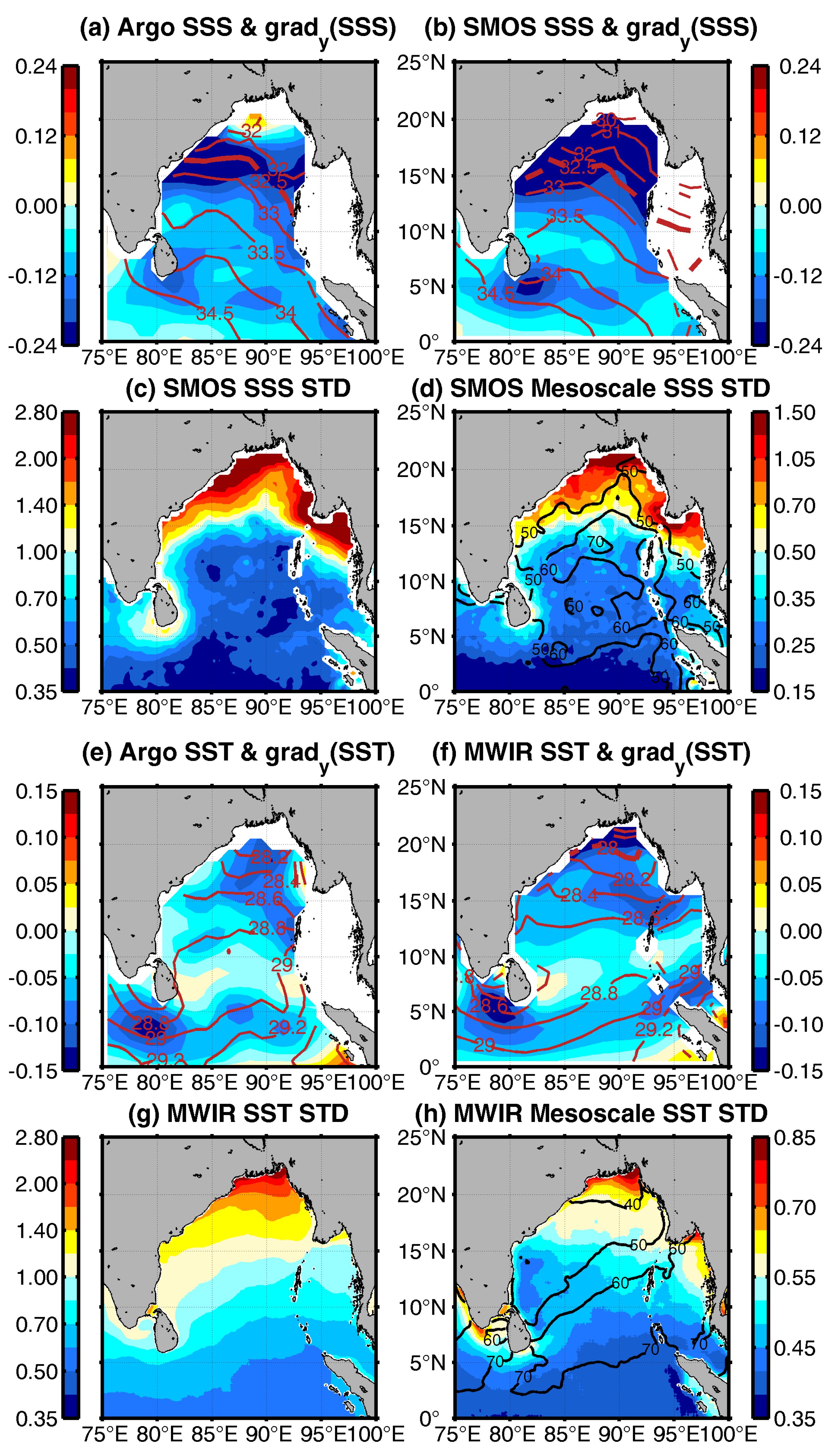
As the thermohaline structure of eddies largely depends on the sign of background horizontal gradients of thermohaline in the upper ocean (e.g., [23,42]), the annual mean characteristics and its variability of SSS and SST are first shown in Figure 2. The SMOS SSS indicated systematically lower values over the bay compared to the values from the Argo data (Figure 2a,b), primarily due to the well−known difference between the skin salinity from the satellite and the 10−m salinity from Argo [26]. However, both datasets showed very similar SSS patterns, with SSS gradually decreasing from 34.5 psu at the equator to below 32 psu in northern bay, highlighting a consistent negative SSS meridional gradient over the entire bay (Figure 2a,b). Much higher SSS meridional gradients with a mean value of approximately –0.23 psu/100 km were located over the higher freshwater content region north to 15°N compared with that (–0.08 psu/100 km) to the south. The full SSS standard deviation indicated that the overall maximum SSS variability (higher than 1.0 psu) coincided with the freshwater region in the northern bay (north to 15°N). Also, 40% to 60% of the total SSS variability was caused by the SSS mesoscale variability (Figure 2c,d). The large mesoscale variability of SSS in northern bay may have been possibly caused by the combined influences of the intense eddy activity [14] and the sharp meridional gradient in SSS created by the considerable amount of freshwater into the northern bay [26].
The mesoscale variability of SST (Figure 2g,h) in each 0.25° grid resembles the corresponding patterns of SSS, indicating much stronger mesoscale variations (0.40 °C vs. 0.25 °C) in the northern bay than in the southern bay. The same negative SST meridional gradient as SSS was likely present in the entire bay, despite a slightly different spatial pattern of SST with two maximum gradients located in northern bay and south to 5°N.
The abovementioned consistent gradients in both SSS and SST over the entire bay led us to take the bay as a whole for a composite analysis of the eddies in Section 4. The composite analysis is discussed in detail in that section.
3.2. Eddy Statistics
Prior to analyzing the three−dimensional structure of mesoscale eddies in the BOB, it was instructive to have a closer look at their mean properties at the sea surface, as identified in the SLA fields. During our primary period of interest from November 2001 to September 2016, there were 624 cyclonic eddies (CEs) and 533 anticyclonic eddies (AEs). The number of CEs was approximately 17% higher than that of AEs, and their mean lifespans were approximately 57 days and 56 days, respectively. Consistent with previous studies [14,16,17], eddy−rich regions with more than four CEs and AEs in each 1° bin were observed to be located at the western boundary, the northern bay, and the Andaman Sea (Figure 3a,b).
The mean amplitudes of the CEs and AEs show a similar spatial pattern (Figure 3c,d). Both measurements indicate that a much larger amplitude (>8 cm) appeared in the western bay than that (<6 cm) in the other regions of the bay, reflecting the high eddy kinetic energy. The main mechanisms, including the strong shear and the baroclinic instability of the EICC and the westward transmitted energy of the Rossby waves into the western basin, are thought to account for the large eddy amplitude and the high eddy kinetic energy in the western boundary [4,15]. The mean radius of both CEs and AEs was larger than 120 km in most parts of the bay, except in the Andaman Sea and the coastal regions, where the mean radius was approximately 100 km, most likely due to the limitation in spatial scale by topography [22]. A remarkable decreasing trend was present in the radius of CEs and AEs with increased latitude, varying substantially from 160–180 km in southern bay to approximately 80 km in the northern part. The definite reduction of radius in the northern bay was also probably caused by the presence of more coastal areas in the area. On average, AEs possessed slightly larger radiuses than CEs, and the most significant differences were present in the western bay, where the anticyclones were approximately 20% larger than cyclones.
Figure 3e,f show the mean eddy velocity propagation field for the CEs and AEs, respectively. The movement speeds indicate similar patterns for both anticyclonic and cyclonic eddies. They were large in the southern bay (~0.1 m s−1), with a comparable magnitude of the rotational velocity to be shown in the following text (i.e., Section 4.2), and decreased sharply in size as latitude increased. Their zonal directions were generally westward because of the well−known quasi−geostrophic theory. The meridional directions were dominated by equatorward in the northern bay (>10°N) and poleward in southern bay (<10°N), with a slightly larger magnitude of meridional velocity for CEs. This mean eddy movement pattern was similar to that found in Chen et al. [14]. As shown in Section 5, the meridional deflection, along with the westward movement of eddies, i.e., the meridional movement of eddies, were responsible for the trapping component of the meridional heat and freshwater transport.
4. Composite Structures and Meridional Fluxes of Eddies
4.1. Horizontal and Vertical Thermohaline Structures
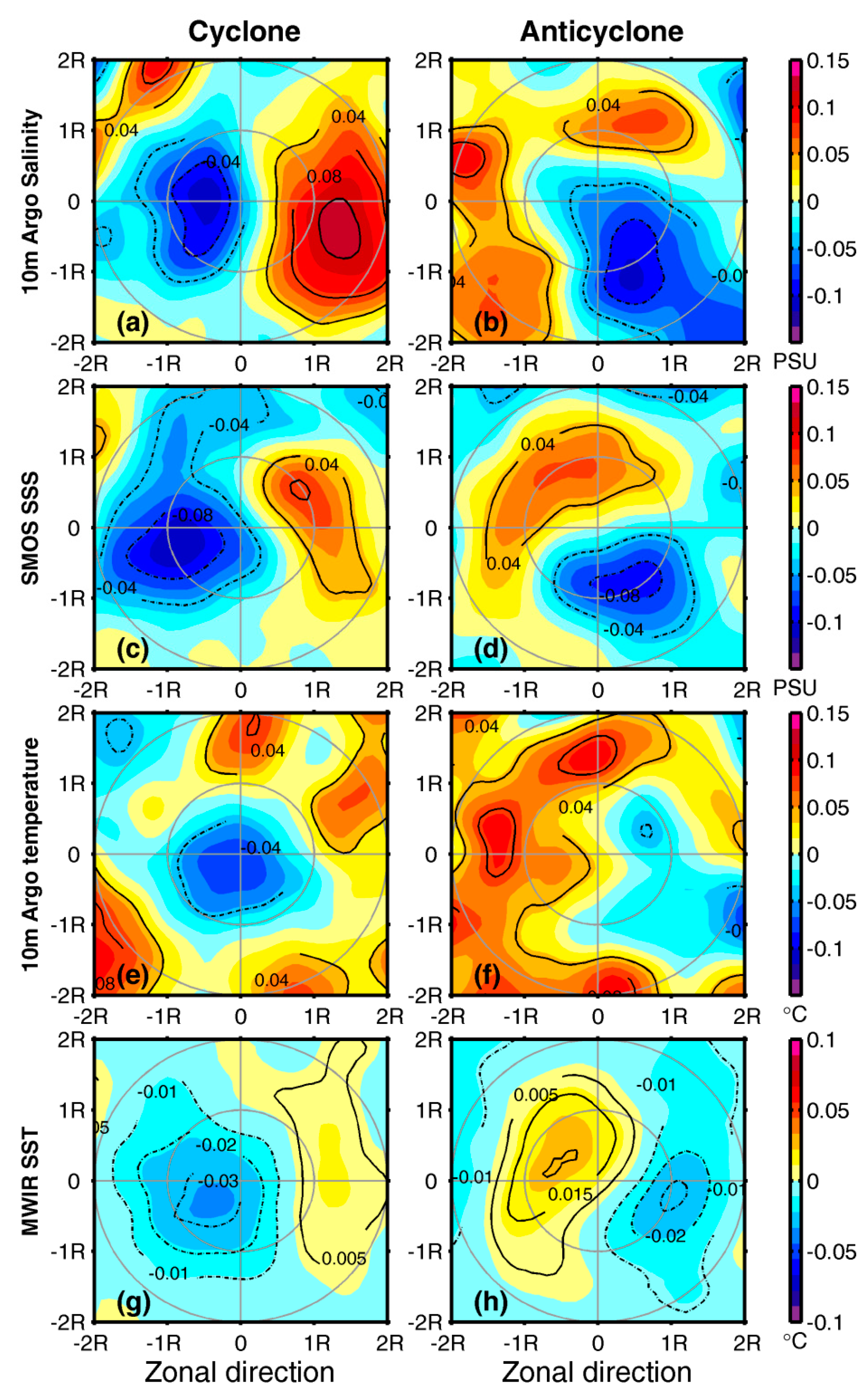
Using the Argo profiles, a composite of the eddy−induced SSS and SST anomalies corresponding to the average cyclonic and anticyclonic eddy are presented in Figure 4a,b,e,f. Satellite−derived SSS and SST signatures of mesoscale eddies (Figure 4c,d,g,h) were also compared with the Argo results. Argo and SMOS produced a similar dipole−like structure (much clearer for the CE) of the SSS anomaly, with a tendency to have opposite SSS anomalies in the leading pole of the eddy compared to those of the trailing pole, although the amplitudes were slightly different. Here, the leading (trailing) pole roughly corresponded to the left (right) half of each composite for salinity, as well as the temperature shown thereinafter [43]. Salt/freshwater eddy cores were surrounded by weaker amplitude negative/positive lobes, which were particularly evident in the composite AEs (Figure 4b). These lobes were reminiscent of wave−like structures or could be indicative of densely packed eddies in the bay. For the composite CE (Figure 4a,c), the Argo (SMOS) SSS anomalies had maximum amplitudes of –0.10 psu (–0.10 psu) in the leading pole and of 0.12 psu (0.08 psu) in the trailing pole. For the composite AE (Figure 4b,d), the Argo (SMOS) SSS anomalies had maximum amplitudes of 0.08 psu (0.06 psu) and –0.10 psu (–0.08 psu) in the leading and trailing pole, respectively.
Remarkably, we can see that the SST anomaly patterns were similar to those of salinity anomalies for either cyclonic or anticyclonic eddies and had a consistent sign: Negative SST anomalies corresponded with negative SSS anomalies and vice versa. Considering that the background SSS and SST gradients were parallel (Figure 2), such dipole structures are consistent with the findings of previous studies [34] that emphasize the leading role of horizontal advection in the background temperature/salinity gradient by the eddy rotational velocities in setting the anomaly patterns. The mean SSS/SST distribution in the study area (Figure 2) showed that such a dipole pattern appeared when a cyclonic eddy advected fresher/colder water from north to south on its western side and saltier/warmer waters from south to north on its eastern side. The opposite was generally true for the composite anticyclonic eddy. However, there were some qualitative differences in the thermohaline structure between the composite cyclonic and anticyclonic eddies. Particularly, in the cyclonic eddy (Figure 4e), the asymmetry between the two poles was much stronger, and the leading pole (i.e., negative SST anomalies) was much closer to the eddy center, likely highlighting that the entrainment processes associated with shoaling thermocline, with the exception of horizontal advection, dominantly lead to the cold pole [23,42]. Similar dipole patterns within eddies has been reported in the previous studies [39,42].
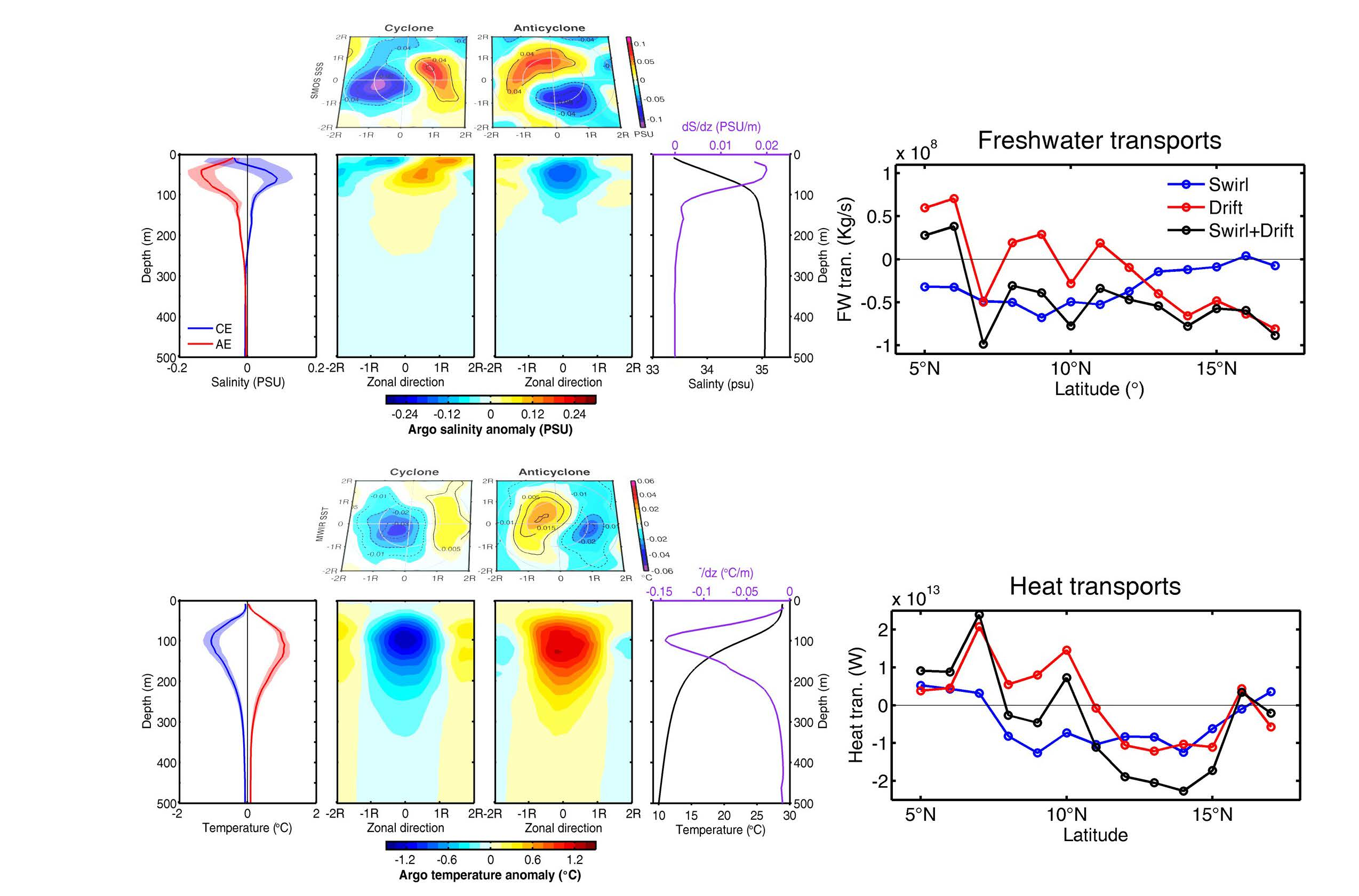
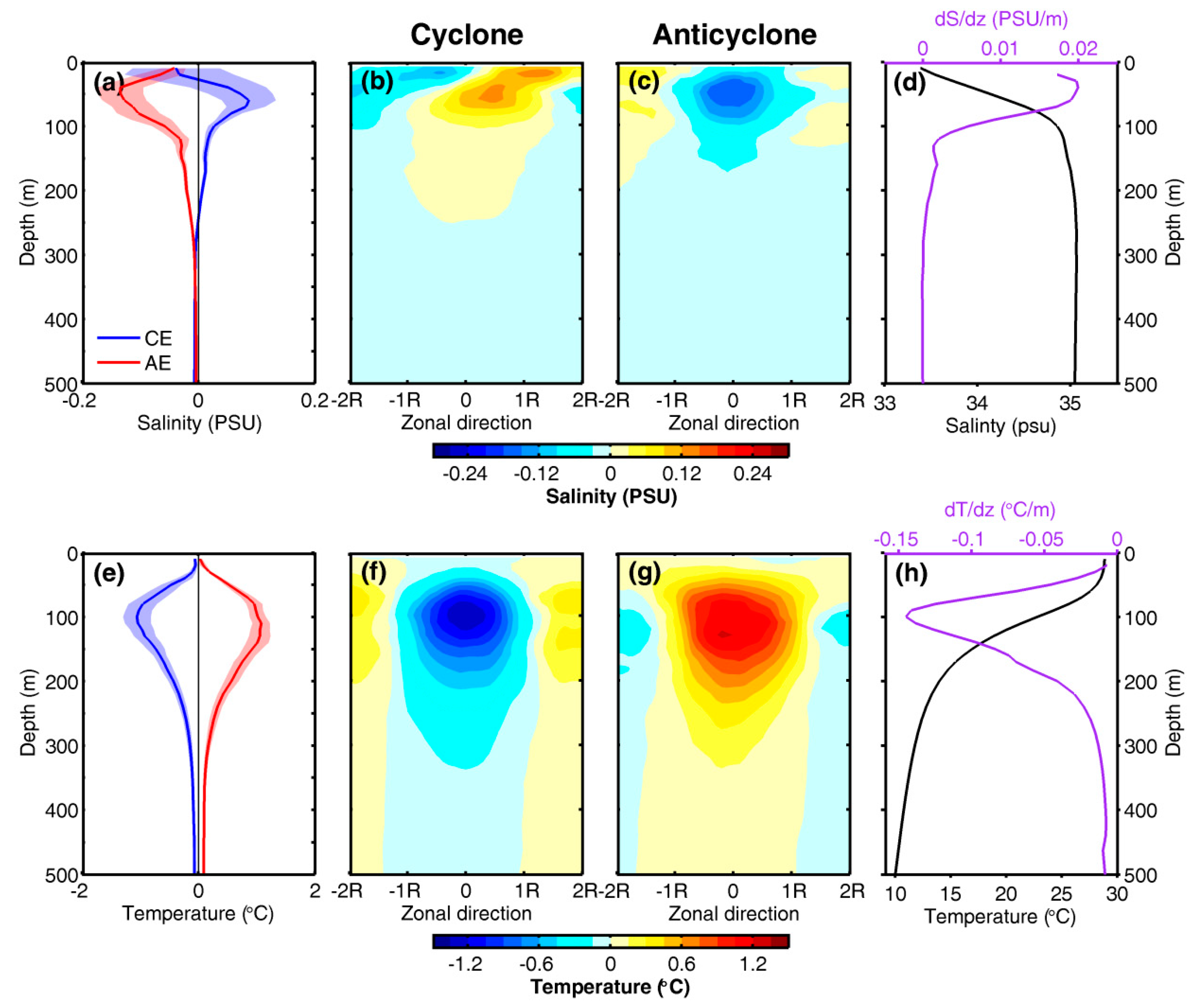
The vertical sections of the salinity/temperature anomalies across the centers of composite eddies are shown in Figure 5. The impacts on salinity of the CEs and AEs can extend to maximum depth of 200 m (Figure 5a–c) because of the relatively strong vertical salinity gradient above that depth. With increasing depth, the surface dipole−like structures of both CEs and AEs shown in Figure 4 lost their strength, and the SSS anomaly converged toward the centers of the eddies (Figure 5a,b). For CEs, a well−pronounced dipole pattern was present above the ~50−m layer, but it showed a monopole structure centered close to the eddy core below the 50−m depth, with its maximum amplitude at approximately 60 m. For AEs, although the dipole pattern of SSS was not as obvious as that in CEs, it also presented a similar decay with depth and becomes undetectable below the ~20−m layer, where the salinity anomalies showed a dominant monopole structure with a maximum amplitude located at 50 m. This outcome occurred in both CEs and AEs because the rotational velocities of the eddies weakened with depth, as shown in Figure 6, and because the horizontal isohalines became flatter with depth (Figure not shown). Thus, the advection effects weakened accordingly with depth. Consequently, with the disappearance of the dipole as depth increased due to the decay of advection, the dominant relevant process was vertical advection, which led to the emergence of a monopole structure centered on the eddy core, which was characterized by saltier and fresher water for the CEs and AEs, respectively. As the vertical salinity gradient first increased gradually and then decreased as depth increased, reaching a maximum value at approximately 50 m (Figure 5d), the vertical advection also reached its maximum at this depth. Therefore, the salinity anomalies for the composite CEs (AEs) with a maximum of 0.1 psu (–0.13 psu) were present between 50 m and 60 m (Figure 5a).
The thermal structure of the CEs (AEs) generally features a cold (warm anomaly) of approximately 1 °C, which peaks within the thermocline layer at approximately 100 m (Figure 5e) and extends downward to the 300−m layer. For the CEs, the monopole structure dominates at the eddies’ full depth, and the temperature anomalies are centrosymmetric at the eddy center, except the near surface (Figure 5f), where the pole deviates slightly southwestward from the eddy center (Figure 4e). Note also that the AEs had a similar monopole structure to that of CEs below the surface layer, with their center deviating slightly westward to the eddy center (Figure 5g), implying that the temperature anomalies at depth were primarily caused by the eddy−induced displacement of the average isopycnal surfaces. A very weak dipole pattern of AEs was only discernible in the near surface layer (above 15 m), which was closely related to the horizontal advection as mentioned above.
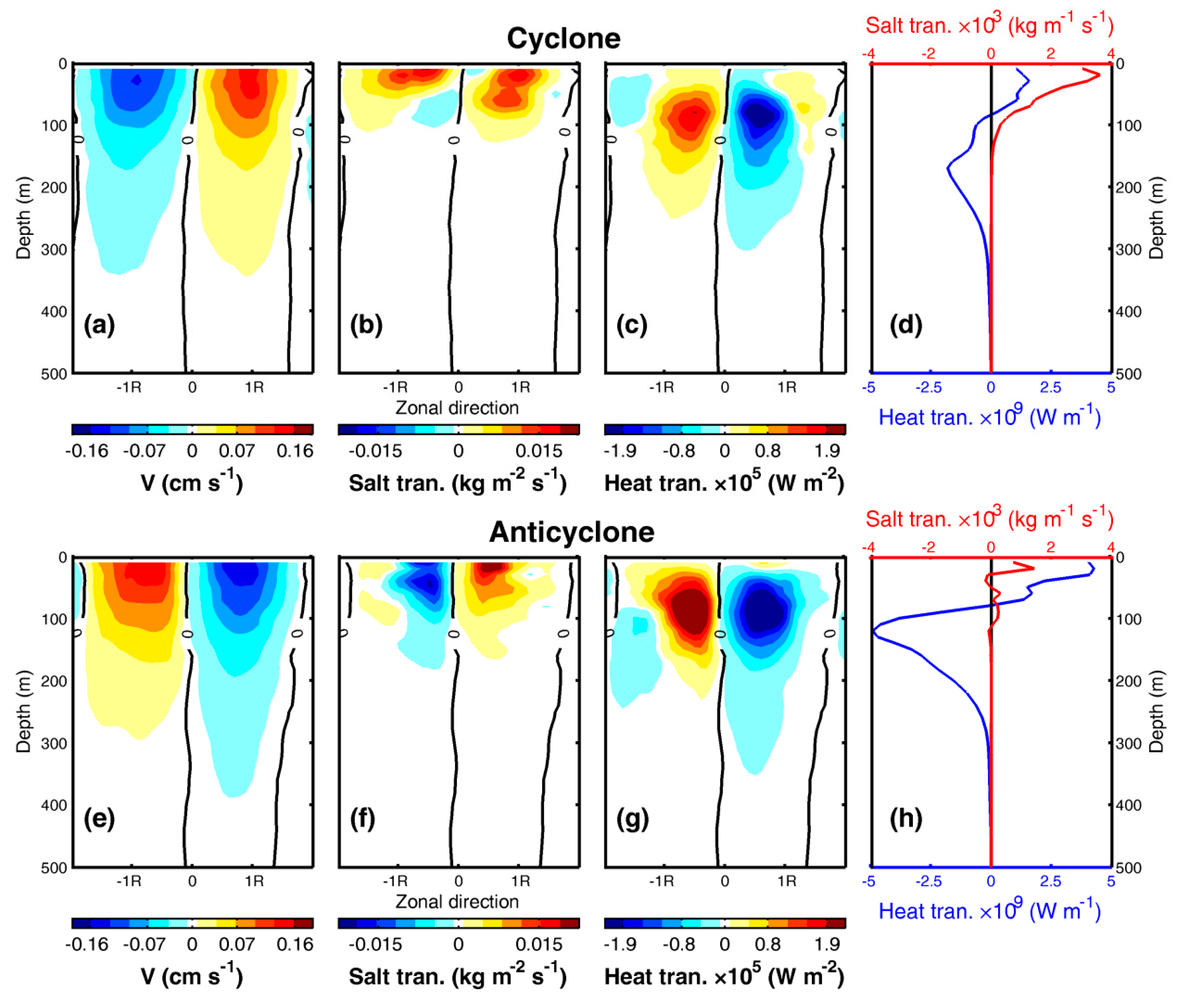
4.2. Meridional Heat and Salt Fluxes
One important point to emphasize from Section 4a is that the eddy−induced thermohaline structure was not centered around the eddy cores in the upper layer, particularly for the surface layer (Figure 4 and Figure 5). As shown in the previous study [42], the asymmetric structure of thermohaline tends to be not in phase with geostrophic current anomalies of the composited eddies, and the systematic phase shifts between eddy thermohaline and velocity anomaly fields lead to net salt/heat fluxes over the eddy wavelength, which is an important contributor to the observed time−varying ocean heat transport [14,31,44].
To clarify the abovementioned effect, first, the geostrophic current structure of composite eddies was examined along zonal sections in Figure 6a,e. Large and coherent eddy velocities mainly appeared above 300 m, while below 300 m, the eddy velocities were hardly discernible. They wrere surface−intensified and decreased with depth. The maximum rotational speeds were observed at a distance of approximately one radius from the eddy centers, with the largest magnitudes of 0.15 m s−1 near the surface. Both cyclonic and anticyclonic eddies had pronounced centrosymmetric structures along the eddy axis, with zero velocity located in the eddy center. However, a closer inspection of Figure 6a,e revealed that the location of maximum velocity showed a weak vertical tilt in the upper 200 m. This vertical tilt in the velocity of the composite eddies can lead to a net heat/salt transport within a geostrophic eddy [23,44].
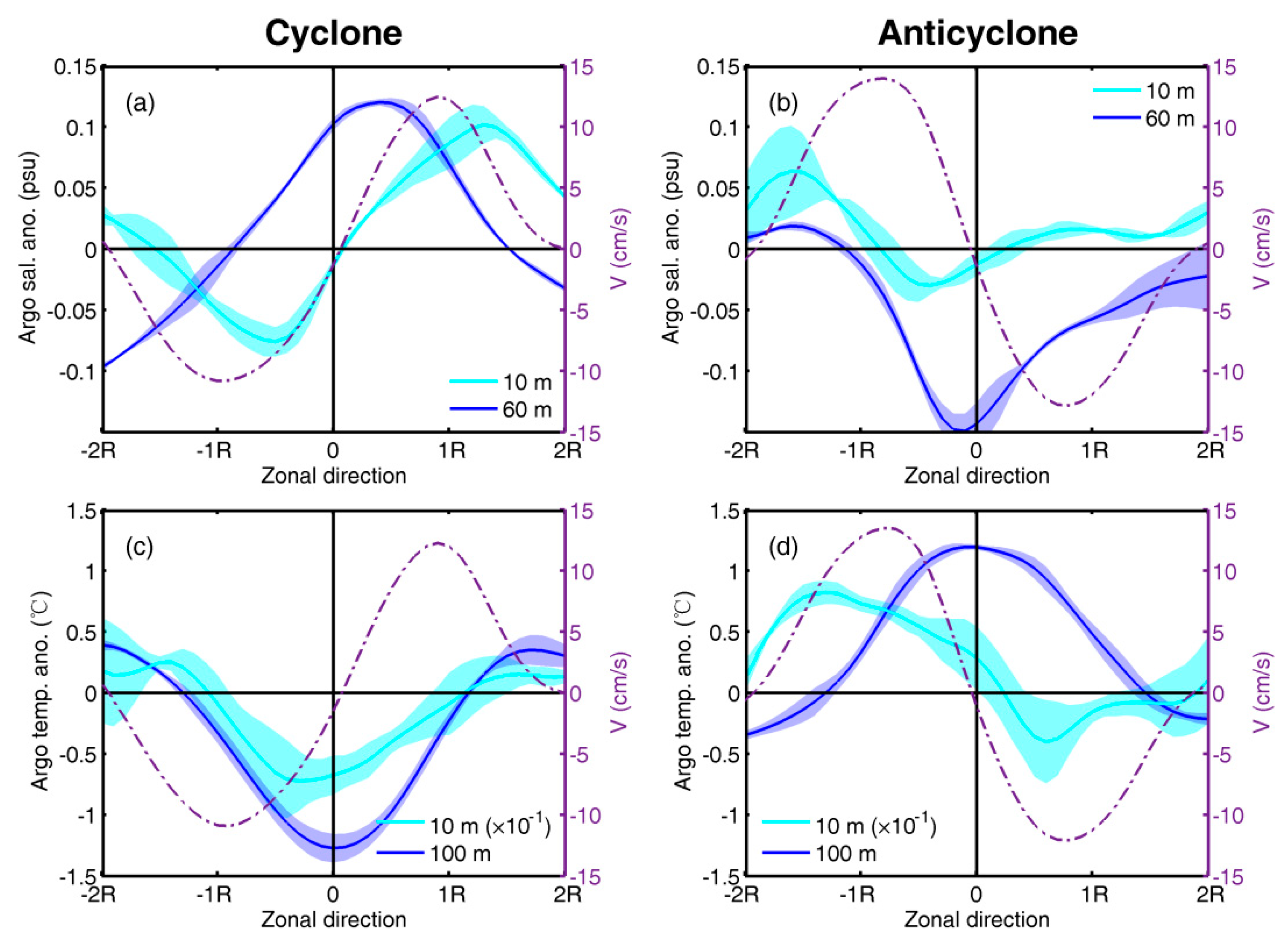
In addition, to examine the phase relationship between the thermohaline and velocity fields, zonal sections at the near surface (10−m layer) for both salinity and temperature and at the core layer (i.e., 60 m for salinity and 100 m for temperature) are shown for comparison (Figure 7). The phase shifts were much more pronounced in the near surface than in the subsurface. In the near surface layer, large phase shifts were mainly caused by the difference between asymmetric thermocline structures (i.e., dipole structure, Figure 4 and Figure 7) and centrosymmetric velocity structures along the eddy axis (Figure 6a,e and Figure 7). At the core layer, although both the thermohaline and velocity showed similar symmetric structures, the phase shifts between them were discernible. For cyclones (anticyclones), both maximum SSSA and SSTA occurred slightly to the east (west) of zero velocity (i.e., the eddy center). As mentioned above, these phase shifts in the thermohaline with respect to the eddy center have been well−noticed in previous work, resulting in a net heat/salt transport over the eddy wavelength due to the rotation of the eddies (e.g., [42]).
The eddy−induced heat and salt fluxes, estimated using Equations (1) and (2), are shown in Figure 6b–d,f–h. A common feature for both the CEs and AEs was that the salt/heat fluxes were mainly concentrated above the halocline (<150 m)/thermocline (<300 m), below which the transport was much smaller and is therefore negligible. The large fluxes in the upper layer are attributed to the relatively large eddy signals in the thermohaline and velocity fields (Figure 5 and Figure 6a,e).
The salt flux of AEs was negative (southward) in the western part and positive (northward) in the eastern part, with a slightly larger northward flux due to the stronger velocity in the eastern part of the upper layers. In contrast, the salt flux induced by CEs was positive (northward) in both the western and eastern parts because of the same sign shown in the SSSA and velocity anomalies for both parts. Consequently, the integrated salt fluxes across the composite CEs and AEs were positive, whereas the magnitude of those induced by AEs was much smaller and shallower than those of CE. Therefore, despite their different magnitudes, both CEs and AEs have the same role in moving salt northward to compensate for the decrease in salinity due to the excess in precipitation over evaporation [1]. The total meridional salt transport induced by the composite CE (AE) was 1.9 × 10⁵ (2.3 × 10⁴) kg s−1.
The heat flux of both CEs and AEs were positive (northward) in the western part of the bay and negative (southward) in the eastern part (Figure 6c,g). From the integrated heat flux across the composite eddies as a function of depth (Figure 6d,h), an important feature was revealed: Both CEs and AEs induced positive transport (poleward) above 100 m and negative values (equatorward) below 100 m, with much larger amplitude in the subsurface. Thus, the total net meridional heat transport induced by the composite CE (AE) was −1.3 × 10¹¹ (−2.6 × 10¹¹) W, which indicates a southward heat flux in the BOB. This feature has been found in a previous study and is typical in the northern hemisphere [41,45], which implies that the eddy not only transports heat toward high latitudes at the surface (i.e., in down−gradient of the isotherms, Figure 2e,f) but also toward low latitudes (i.e., up−gradient) at subsurface layers.
5. Discussion
5.1. Seasonal Variability of Eddy Thermohaline Structure
Consistent with a previous study (e.g., [42,46]), our results showed that the mean eddy structure strongly depends on the temperature/salinity fields (Figure 4 and Figure 5). Recently, Zu et al. found that in the South China Sea, a strong annual cycle of hydrographic background can induce remarkable seasonal variability in the eddy thermohaline structure [46].
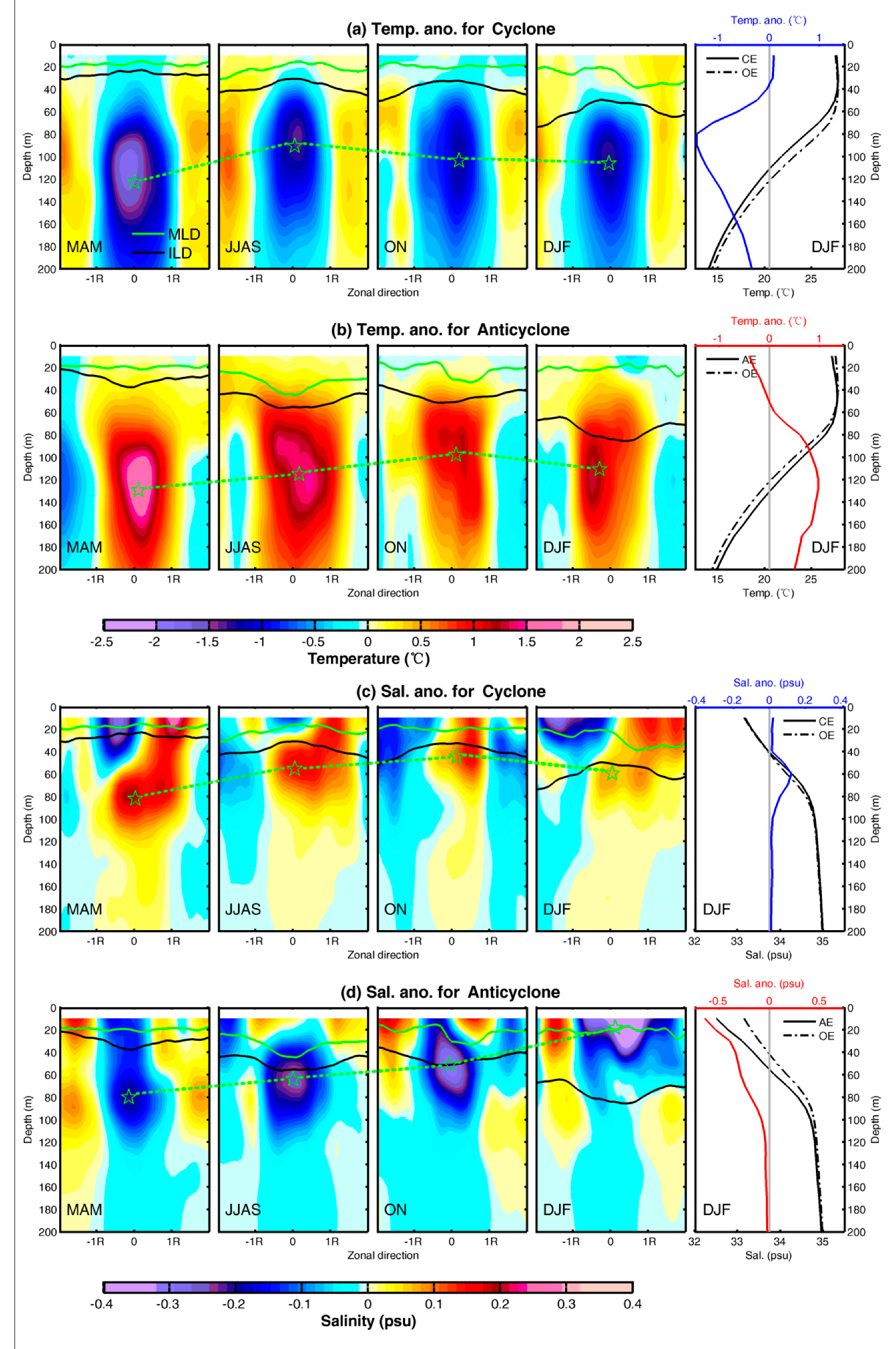
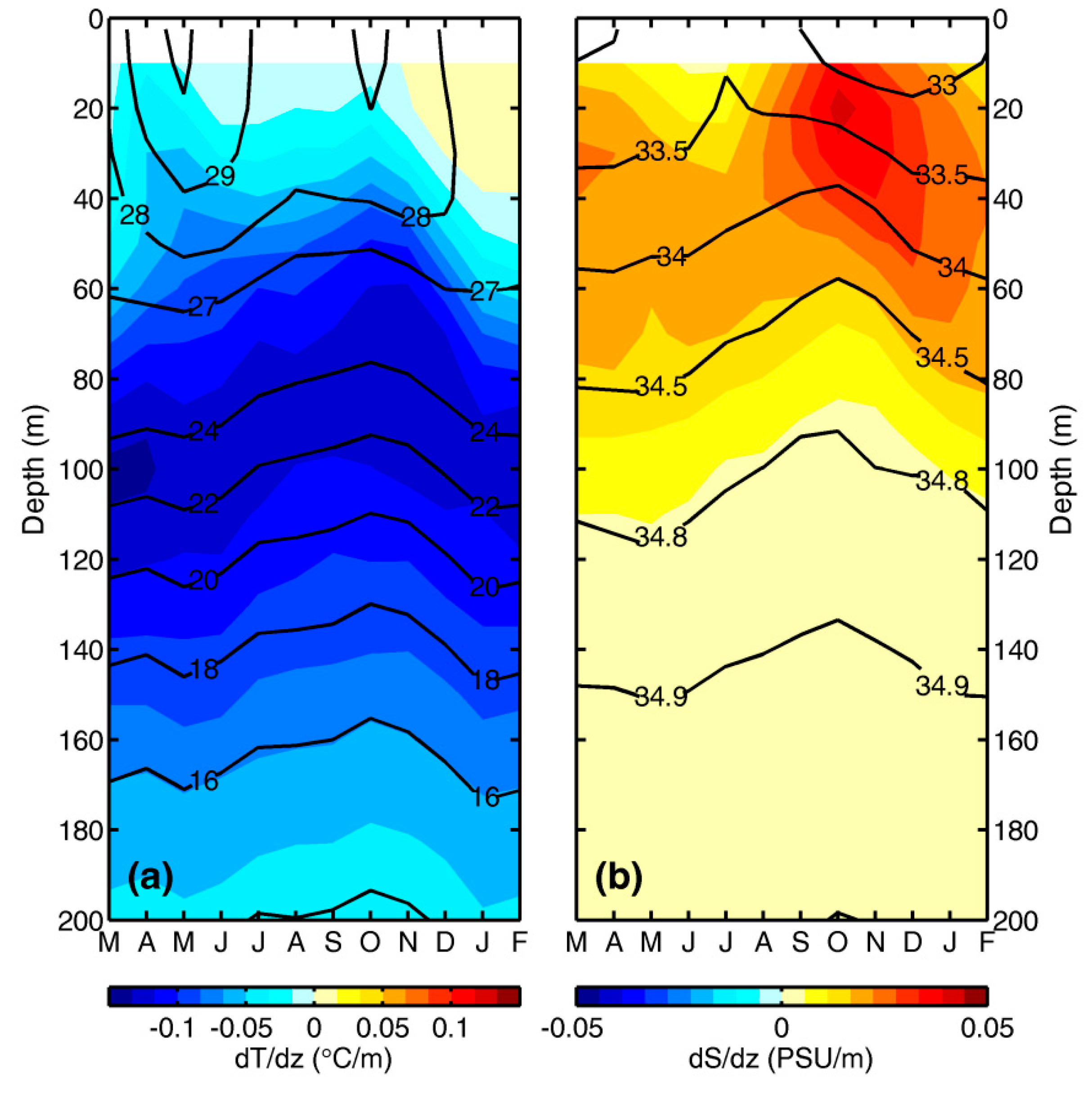
To investigate the seasonal differences in eddy thermohaline structure in the bay, we created composites of eddy structures (Figure 8) for spring (March to May), summer (June to September), fall (October and November), and winter (December to February). From the anomalous temperature structures induced by eddies (Figure 8a,b), our results showed that the composite CE (AE) can induce cold (warm) temperature anomalies with an intensified subsurface magnitude. Both had a single−core vertical structure with the core located at a depth ranging from 100 m to 130 m, a level corresponding to the seasonal thermocline characterized by temperature ranges between 20 °C and 22 °C (Figure 9a). The cores of the CEs and AEs reached the lowest depths and the magnitude of temperature anomalies was largest (~2.5 °C) in the spring due to the relatively deep thermocline and the strong vertical gradient of temperature compared to other seasons (Figure 9a).
A closer inspection of Figure 9a,b revealed a very unique feature: During winter, the CE can induce warming anomalies in the mixed layer, which is in contrast with the features seen in other seasons. This reverse structure was closely associated with the temperature inversion layer within the barrier layers (i.e., a warm layer sandwiched between the surface and subsurface colder waters) that occurs in winter [29]. Under the temperature inversion condition, the warmer and saltier water from the BL was pumped upward and warms the mixed layer of the CEs (Figure 8, right panels), consequently resulting in surface warming. This result implies that the entrainment processes associated with CEs would be an important venue for the release of subsurface warm water in the bay during winter.
For the eddy−induced anomalous salinity (Figure 8c,d), the subsurface intensified single−core vertical structure of the CEs and AEs were only present in spring, summer, and fall, whereas the surface intensified structure was remarkable during winter. Similar to temperature anomalies, the salinity core of CEs and AEs was in seasonal halocline with a depth ranging from 60 m to 80 m. It reached the deepest in the spring due to the relatively deeper halocline compared to other seasons (Figure 9b). In the near surface, a pronounced dipole structure of salinity was present in both CEs and AEs, particularly for CEs, and it can extend to approximately 50 m.
5.2. The Estimation of Eddy Thermohaline Transport in the BOB
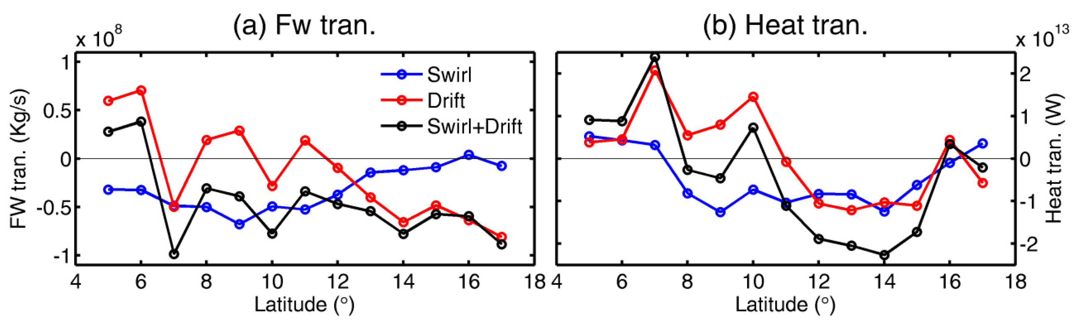
In Section 4, the fluxes of heat and salt for a single “composite” eddy were estimated using its three−dimensional structure (Figure 6). To quantify its role in the basin−scale balance of heat and salt in the BOB, we used a similar approach to that of Melnichenko et al. [42]. We reconstructed the composite of eddy−induced temperature and salinity anomalies in the 4° latitude bins centered on a 1° latitude north to 5°N and extending zonally throughout the bay. We then estimated the freshwater and heat flux in upper 300 m by the composited eddy in each 1° latitude, which represented the meridional freshwater flux and heat transport per a composite eddy as a function of latitude. The swirl and drift components of heat and salt transport by a composite eddy in each latitude bin were estimated using Equations (3)–(6). These estimated fluxes were further multiplied by the average number of eddies (4–5) that were present simultaneously in each latitude bin to obtain eddy transport across each latitude (Figure 10).
As shown in Figure 10b, the swirl heat component was comparable to the drift component, and both contributed roughly equally to the total eddy fluxes. The total heat transport was poleward in the southern bay (south to 10°N) with a mean value of 0.01 PW, whereas it turned equatorward in most regions of the northern bay (north to 10°N), with a mean value of approximately –0.013 PW.
The total eddy freshwater transport was equatorward in most of the bay (Figure 10a). The poleward freshwater transport was only present in the south to 6°N, primarily caused by poleward drift transport associated with the northward movement of eddies there (Figure 3e,f). The eddy−induced mean equatorward freshwater transport was 0.46 × 10⁸ kg s−1 (i.e., 0.046 Sv). This number should be compared with the annual mean net input of freshwater due to the evaporation minus the precipitation (E−P) and the river discharge of 4050 km3 yr−1 (i.e., 0.13 Sv, [47]). Therefore, our estimates suggest that the contribution of mesoscale eddies to the freshwater flux export equatorward out of the bay was approximately 35% to balance for the net input of freshwater into the bay due to the excess of precipitation over evaporation.
Note that the eddy dataset used in our calculations only included the long−lifetime (>28 days) eddies, and thus excluded the possible contributions of short−lived eddies to the volume, heat, and freshwater budgets. Our results do indicate, nonetheless, that mesoscale eddies can influence the heat and freshwater budgets of the bay. In particular, we showed that eddy−induced meridional transport is an important mechanism for maintaining the bay’s salinity levels in spite of a large net freshwater input, which is comparable in magnitude to that of the freshwater advection associated with the large−scale circulation [47,48].
6. Conclusions
In this paper, we systematically explored the thermohaline structure and transport characteristics of mesoscale eddies in the Bay of Bengal (BOB) by composite analysis using Argo profiles and satellite data. Eddy signals in temperature and salinity anomalies were mainly confined to the upper 300 m. Both the composite CE and AE were generally intensified in the subsurface and had a single−core vertical structure. The maximum temperature and salinity anomalies of the eddy core were ±1.2 °C and ±0.1 psu, located at approximately 100 m and 50 m, respectively, with negative (positive) values for the CE (AE) and operating in opposite directions for salinity. Forced by the combined impacts of horizontal advection and vertical entrainment in the background temperature/salinity gradient by the eddy velocity field, the horizontal thermohaline structure of the composite eddy was generally characterized as having a dominant dipole structure near the surface and of a monopole structure in the subsurface.
Both the temperature and salinity core of the CEs and AEs showed pronounced seasonal variation, reaching much lower depths during spring compared to other seasons. The deepening in the core of eddy is primarily caused by the relatively deep thermocline and halocline during spring. In addition, a unique warming anomaly induced by the CE was present in the mixed layer during winter, which was due to the entrainment of warmer water from the BL by the CE. This result implies that CE−induced upward heat pumping would be an important way for the release of warmer water in the thick BL during winter.
The meridional heat and salt transport for the composite eddies were then estimated using the thermohaline and rotational velocity fields (i.e., the swirl heat/salt transport). The mean composite CE and AE caused a consistent southward swirl heat transport with values of −1.3 × 10¹¹ and −2.6 × 10¹¹ W and induced consistent northward swirl salt transport of 1.9 × 10⁵ and 2.3 × 10⁴ kg s−1. This net heat and freshwater transport produced by eddies was due to the phase shift between the eddy−induced thermohaline and velocity anomalies, and thus has important implications for the regional heat balance and hydrological cycle in the BOB.
To further quantify their roles in freshwater and heat balance in the bay, we reconstructed the composite averages of eddy−induced temperature and salinity anomalies in 4° latitude bins centered on a 1° latitude grid throughout the bay. The total heat and freshwater transport (including the swirl component and the drift component) was then estimated by a composite eddy in each latitude bin over a one−year period. The result showed that the total eddy heat transport was poleward (equatorward) south (north) to 10°N, with a mean value of 0.01 PW and –0.013 PW, implying eddy−induced heat convergence in the area. The consistent southward meridional transport of freshwater was present north to 6°N with a mean value of 0.046 Sv, and freshwater exports out of the bay were approximately 35% of the annual net freshwater input from the local precipitation and river discharge. Thus, our estimates imply that mesoscale eddies’ contribution to the salinity balance of the bay is comparable to that of the large−scale circulation.
Author Contributions
Conceptualization, Y.Q.; methodology, X.L. and Y.Q.; validation, Y.Q. and X.L.; formal analysis, X.L.; data curation, X.L. and Y.Q.; writing—original draft preparation, Y.Q. and X.L.; writing—review and editing, Y.Q. and D.S.; visualization, X.L; funding acquisition, Y.Q. All authors listed have reviewed and approved the final version of this manuscript.
Funding
This research is jointly supported by grants from the Scientific Research Foundation of Third Institute of Oceanography, Ministry of Natural Resources (Grants No. 2017012 and 2018001), the State Oceanic Administration Program on Global Change and Air−Sea interactions (Grants No. GASI−IPOVAI−02, GASI−IPOVAI−03), the National Key Research and Development Program of China (Grants No. 2016YFC1401003 and 2016YFC1402607), and a scholarship from the China Scholarship Council (Grant No. 201604180033).
Acknowledgments
We would like to thank the reviewers for their time spent on reviewing our manuscript and their comments helping us improving the article. The altimeter the Mesoscale Eddy Trajectory Atlas products used here were produced by SSALTO/DUACS and distributed by AVISO+ (https://www.aviso.altimetry.fr/) with support from CNES, in collaboration with Oregon State University with support from NASA.
Conflicts of Interest
The authors declare no conflict of interest.
References
- Varkey, M.J.; Murty, V.S.N.; Suryanarayana, A. Physical oceanography of the Bay of Bengal and Andaman Sea. Oceanogr. Mar. Biol. Annu. Rev. 1996, 34, 1–70. [Google Scholar]
- Potemra, J.T.; Luther, M.E.; O’Brien, J.J. The seasonal circulation of the upper ocean in the Bay of Bengal. J. Geophys. Res. Oceans 1991, 96, 12667–12683. [Google Scholar] [CrossRef] [Green Version]
- Babu, M.T.; Sarma, Y.V.B.; Murty, V.S.N.; Vethamony, P. On the circulation in the Bay of Bengal during northern spring inter−monsoon (March–April 1987). Deep Sea Res. Part II 2003, 50, 855–865. [Google Scholar] [CrossRef]
- Somayajulu, Y.K.; Murty, V.S.N.; Sarma, Y.V.B. Seasonal and inter−annual variability of surface circulation in the Bay of Bengal from TOPEX/Poseidon altimetry. Deep Sea Res. Part II 2003, 50, 867–880. [Google Scholar] [CrossRef]
- Shankar, D.; McCreary, J.P.; Han, W.; Shetye, S.R. Dynamics of the East India Coastal Current. 1. Analytic solutions forced by interior Ekman pumping and local alongshore winds. J. Geophys. Res. Oceans 1996, 101, 13975–13991. [Google Scholar] [CrossRef]
- Ramasastry, A.A.; Balaramamurty, C. Thermal fields and oceanic circulation along the east coast of India. Proc. Ind. Acad. Sci. Sect. B 1957, 46, 293–323. [Google Scholar]
- Rao, D.P.; Sastry, J.S. Circulation and distribution of some hydrographical properties during the late winter in the Bay of Bengal Mahasagar. Bull. Natl. Inst. Oceanogr. 1981, 14, 1–16. [Google Scholar]
- Babu, M.T.; Kumar, P.S.; Rao, D.P. A subsurface cyclonic eddy in the Bay of Bengal. J. Mar. Res. 1991, 49, 403–410. [Google Scholar] [CrossRef]
- Hacker, P.; Firing, E.; Hummon, J.; Gordon, A.L.; Kindle, J.C. Kindle. Bay of Bengal currents during the Northeast Monsoon. Geophys. Res. Lett. 1998, 25, 2769–2772. [Google Scholar] [CrossRef] [Green Version]
- Singh, A.; Gandhi, N.; Ramesh, R.; Prakash, S. Role of cyclonic eddy in enhancing primary and new production in the Bay of Bengal. J. Sea Res. 2015, 97, 5–13. [Google Scholar] [CrossRef]
- Prasanna Kumar, S.; Nuncio, M.; Narvekar, J.; Kumar, A.; Sardesai, D.S.; De Souza, S.N.; Gauns, M.; Ramaiah, N.; Madhupratap, M. Are eddies nature’s trigger to enhance biological productivity in the Bay of Bengal? Geophys. Res. Lett. 2004, 31, L07309. [Google Scholar] [CrossRef] [Green Version]
- Sanilkumar, K.V.; Kuruvilla, T.V.; Jogendranath, D.; Rao, R.R. Observations of the Western boundary current of the Bay of Bengal from a hydrographic survey during March 1993. Deep Sea Res. Part I 1997, 44, 135–145. [Google Scholar] [CrossRef]
- Sarma, Y.V.B.; Rao, E.R.; Saji, P.K.; Sarma, V.V.S.S. Hydrography and circulation of the Bay of Bengal during withdrawal phase of the southwest Monsoon. Oceanol. Acta 1999, 22, 453–471. [Google Scholar] [CrossRef] [Green Version]
- Chen, G.; Gan, J.; Xie, Q.; Chu, X.; Wang, D.; Hou, Y. Eddy heat and salt transports in the South China Sea and their seasonal modulations. J. Geophys. Res. Oceans 2012, 117, C05021. [Google Scholar] [CrossRef] [Green Version]
- Chen, G.; Li, Y.; Xie, Q.; Wang, D. Origins of Eddy Kinetic Energy in the Bay of Bengal. J. Geophys. Res. Oceans 2018, 123, 2097–2115. [Google Scholar] [CrossRef]
- Cui, W.; Yang, J.G.; Ma, Y. A statistical analysis of mesoscale eddies in the Bay of Bengal from 22–year altimetry data. Acta Oceanol. Sin. 2016, 35, 16–27. [Google Scholar] [CrossRef]
- Cheng, X.; McCreary, J.P.; Qiu, B.; Qi, Y.; Du, Y.; Chen, X. Dynamics of eddy generation in the central Bay of Bengal. J. Geophys. Res. Oceans 2018, 123, 6861–6875. [Google Scholar] [CrossRef]
- Wang, G.; Su, J.; Chu, P.C. Mesoscale eddies in the South China Sea observed with altimeter data. Geophys. Res. Lett. 2003, 30. [Google Scholar] [CrossRef] [Green Version]
- Chaigneau, A.; Le Texier, M.; Eldin, G.; Grados, C.; Pizarro, O. Vertical structure of mesoscale eddies in the eastern South Pacific Ocean: A composite analysis from altimetry and Argo profiling floats. J. Geophys. Res. Oceans 2011, 116, C11025. [Google Scholar] [CrossRef]
- Hu, J.; Gan, J.; Sun, Z.; Zhu, J.; Dai, M. Observed three−dimensional structure of a cold eddy in the southwestern South China Sea. J. Geophys. Res. Oceans 2011, 116. [Google Scholar] [CrossRef]
- Yang, G.; Wang, F.; Li, Y.; Lin, P. Mesoscale eddies in the northwestern subtropical Pacific Ocean: Statistical characteristics and three−dimensional structures. J. Geophys. Res. Oceans 2013, 118, 1906–1925. [Google Scholar] [CrossRef]
- Yang, G.; Yu, W.; Yuan, Y.; Zhao, X.; Wang, F.; Chen, G.; Liu, L.; Duan, Y. Characteristics, vertical structures, and heat/salt transports of mesoscale eddies in the southeastern tropical Indian Ocean. J. Geophys. Res. Oceans 2015, 120, 6733–6750. [Google Scholar] [CrossRef]
- Amores, A.; Melnichenko, O.; Maximenko, N. Coherent mesoscale eddies in the North Atlantic subtropical gyre: 3−D structure and transport with application to the salinity maximum. J. Geophys. Res. Oceans 2017, 122, 23–41. [Google Scholar] [CrossRef]
- Delcroix, T.; Chaigneau, A.; Soviadan, D.; Boutin, J.; Pegliasco, C. Eddy−induced salinity changes in the tropical Pacific. J. Geophys. Res. Oceans 2019, 124. [Google Scholar] [CrossRef]
- Ansorge, I.J.; Jackson, J.M.; Reid, K.; Durgadoo, J.V.; Swart, S.; Eberenz, S. Evidence of a southward eddy corridor in the south−west Indian ocean. Deep Sea Res. Part II 2014, 119, 69–76. [Google Scholar] [CrossRef]
- Garreau, P.; Dumas, F.; Louazel, S.; Correard, S.; Fercocq, S.; Le Menn, M.; Serpette, A.; Garnier, V.; Stegner, A.; Le Vu, B.; et al. PROTEVS−MED field experiments: Very High−Resolution Hydrographic Surveys in the Western Mediterranean Sea. Earth Syst. Sci. Data Discuss 2019. [Google Scholar] [CrossRef] [Green Version]
- Dandapat, S.; Chakraborty, A. Mesoscale Eddies in the Western Bay of Bengal as Observed From Satellite Altimetry in 1993–2014: Statistical Characteristics, Variability and Three−Dimensional Properties. IEEE J. STARS 2016, 9, 5044–5054. [Google Scholar] [CrossRef]
- Lin, X.; Qiu, Y.; Cha, J.; Guo, X. Assessment of Aquarius sea surface salinity with Argo in the Bay of Bengal. Int. J. Remote Sens. 2019, 40, 1–19. [Google Scholar] [CrossRef]
- Thadathil, P.; Suresh, I.; Gautham, S.; Prasanna Kumar, S.; Lengaigne, M.; Rao, R.R.; Neetu, S.; Hegde, A. Surface layer temperature inversion in the Bay of Bengal: Main characteristics and related mechanisms. J. Geophys. Res. Oceans 2016, 121, 5682–5696. [Google Scholar] [CrossRef]
- Volkov, D.L.; Lee, T.; Fu, L.L. Eddy−induced meridional heat transport in the ocean. Geophys. Res. Lett. 2008, 35. [Google Scholar] [CrossRef] [Green Version]
- Zhang, Z.; Wang, W.; Qiu, B. Oceanic mass transport by mesoscale eddies. Science 2014, 345, 322–324. [Google Scholar] [CrossRef] [PubMed]
- Cotroneo, Y.; Budillon, G.; Fusco, G.; Spezie, G. Cold core eddies and fronts of the Antarctic Circumpolar Current south of New Zealand from in situ and satellite data. J. Geophys. Res. Oceans 2013, 118, 2653–2666. [Google Scholar] [CrossRef]
- Duacs/AVISO+. Mesoscale Eddy Trajectory Atlas Product Handbook; SALP−MU−P−EA−23126−CLS; AVISO+: Ramonville St Agne, France, 2017. [Google Scholar]
- Chelton, D.B.; Schlax, M.G.; Samelson, R.M. Global observations of nonlinear mesoscale eddies. Prog. Oceanogr. 2011, 91, 167–216. [Google Scholar] [CrossRef]
- Wong, A.P.; Johnson, G.C.; Owens, W.B. Delayed−mode calibration of autonomous CTD profiling float salinity data by theta−S climatology. J. Atmos. Ocean. Technol. 2003, 20, 308–318. [Google Scholar] [CrossRef] [Green Version]
- Gentemann, C.L.; Wentz, F.J.; DeMaria, M. Near real time global optimum interpolated microwave SSTs: Applications to hurricane intensity forecasting. In Proceedings of the 27th Conference on Hurricanes and Tropical Meteorology, Monterey, CA, USA, 28 April 2006; pp. 23–28. [Google Scholar]
- Boutin, J.; Vergely, J.L.; Marchand, S.; d’Amico, F.; Hasson, A.; Kolodziejczyk, N.; Reul, N.; Reverdin, G.; Vialard, J. New SMOS Sea Surface Salinity with reduced systematic errors and improved variability. Remote Sens. Environ. 2018, 214, 115–134. [Google Scholar] [CrossRef] [Green Version]
- Roemmich, D.; Gilson, J. The 2004–2008 mean and annual cycle of temperature, salinity, and steric height in the global ocean from the Argo Program. Prog. Oceanogr. 2009, 82, 81–100. [Google Scholar] [CrossRef]
- Chelton, D.B.; Gaube, P.; Schlax, M.G.; Early, J.J.; Samelson, R.M. The influence of nonlinear mesoscale eddies on near−surface oceanic chlorophyll. Science 2011, 334, 328–332. [Google Scholar] [CrossRef]
- Hausmann, U.; Czaja, A. The observed signature of mesoscale eddies in sea surface temperature and the associated heat transport. Deep Sea Res. Part I 2012, 70, 60–72. [Google Scholar] [CrossRef]
- Dong, C.; McWilliams, J.; Liu, Y.; Chen, D. Global heat and salt transports by eddy movement. Nat. Commun. 2014, 5, 3294. [Google Scholar] [CrossRef] [Green Version]
- Sun, B.W.; Liu, C.; Wang, F. Global meridional eddy heat transport inferred from Argo and altimetry observations. Sci. Rep. 2019, 9, 1345. [Google Scholar] [CrossRef] [Green Version]
- Melnichenko, O.; Amores, A.; Maximenko, N.; Hacker, P.; Potemra, J. Signature of mesoscale eddies in satellite sea surface salinity data. J. Geophys. Res. Oceans 2017, 122, 1416–1424. [Google Scholar] [CrossRef]
- Roemmich, D.; Gilson, J. Eddy transport of heat and thermocline waters in the North Pacific: A key to interannual/decadal climate variability? J. Phys. Oceanogr. 2011, 31, 675–687. [Google Scholar] [CrossRef]
- Griffies, S.M.; Winton, M.; Anderson, W.G.; Benson, R.; Delworth, T.L.; Dufour, C.O.; Wittenberg, A.T. Impacts on Ocean Heat from Transient Mesoscale Eddies in a Hierarchy of Climate Models. J. Clim. 2015, 28, 952–977. [Google Scholar] [CrossRef]
- Zu, Y.C.; Sun, S.W.; Zhao, W.; Li, P.L.; Liu, B.C.; Fang, Y.; Samah, A.A. Seasonal characteristics and formation mechanism of the thermohaline structure of mesoscale eddy in the South China Sea. Acta Oceanol. Sin. 2019, 38, 29–38. [Google Scholar] [CrossRef]
- Sengupta, D.; Bharath Raj, G.N.; Shenoi, S.S.C. Surface freshwater from Bay of Bengal runoff and Indonesian Throughflow in the tropical Indian Ocean. Geophys. Res. Lett. 2006, 33, L22609. [Google Scholar] [CrossRef] [Green Version]
- Vinayachandran, P.N.; Shankar, D.; Vernekar, S.; Sandeep, K.K.; Amol, P.; Neema, C.P.; Chatterjee, A. A summer monsoon pump to keep the Bay of Bengal salty. Geophys. Res. Lett. 2013, 40, 1777–1782. [Google Scholar] [CrossRef]
Figure 1.
Bathymetric chart of the Bay of Bengal (color shading) and seasonal surface currents (vector) for (a) January and (b) July from Ocean Surface Currents Analysis Real−time (OSCAR) data during the period of 1992–2017.
Figure 1.
Bathymetric chart of the Bay of Bengal (color shading) and seasonal surface currents (vector) for (a) January and (b) July from Ocean Surface Currents Analysis Real−time (OSCAR) data during the period of 1992–2017.

Figure 2.
Annual mean sea surface salinity (SSS; contours; psu) and its meridional gradient (color shading; psu/100 km) computed from (a) monthly Argo salinity at 10 m during November 2001 and September 2016, and (b) monthly SMOS SSS for the period of 2010 and 2017. SMOS SSS standard deviation values (color shading) denoting (c) the full and (d) the mesoscale−only variability (color shading) and its percentage of the full variability (contours). (e–h) are the same as (a–d), but derived from Argo and MWIR SST, respectively.

Figure 3.
Climatological distribution of cyclonic eddy (CE) in each 1° bin (a) the number of the CE genesis, together with (c) its radii (contours, km) and amplitude (color shading, cm), and (e) the propagation velocity vector of CE and its meridional component (shading) with positive value denoted northward. (b,d,f) are the same as (a,c,e), but for the anticyclonic eddy (AE), respectively. (g) Latitudinal distribution for meridional component of propagation velocity of CE (blue curve) and AE (red curve).

Figure 4.
Composite average of (a,b) salinity and (e,f) temperature anomalies at the 10−m layer from Argo data associated with cyclonic (left columns) and anticyclonic (right columns) eddies. (c,d) and (g,h) are the same as (a,b) and (e,f), respectively, but for SMOS SSS and MWIR SST for a comparison with Argo observations. The grey solid lines in all panels correspond to one time and twice the eddy radius. The positive directions are eastward and northward, respectively. The horizontal and vertical axes in all panels are, respectively, the latitudinal and meridional distances from the eddy center measured by normalized eddy radius (R).

Figure 5.
Mean vertical profiles of (a) salinity anomalies averaged within first one radius of the composite CEs (blue curve) and AEs (red curve). Vertical sections of the salinity anomalies across the center of (b) the composite CEs and (c) AEs, with the horizontal axis representing the latitudinal distances from the eddy center given in the normalized eddy radius (R), and its positive direction is eastward. (d) Mean salinity profile (black curve) and gradients of salinity (purple curve) based on all the Argo profiles outside the eddy in the bay. (e–h) are the same as (a–c), respectively, except for the temperature anomaly. The shaded areas in (a,d) denote the range of one standard deviation for the composite profiles.

Figure 6.
Cross−sections cutting through the center of composite CE for (a) meridional geostrophic current anomaly, (b) mean salt flux, (c) mean heat flux, and (d) integrated salt (red curve) and heat (blue curve) fluxes across the eddy within its twice radius. (e–h) are the same as (a–d), respectively, but for the composite AE.

Figure 7.
Zonal profile (through the center of composite CE) for (a) salinity anomaly at 10 m (SSSA, light blue solid curve) and at 60 m (deep blue solid curve), (c) temperature anomaly at 10 m (SSTA, light blue solid curve) and at 100 m (deep blue solid curve). (b,d) are the same as (a,c), respectively, but for composite AE. In each panel, meridional component of surface geostrophic velocity (purple dash curve) associated with the composite eddy is also overlaid to highlight phase shifts of both SSSA and SSTA compared to the eddy meridional velocity. The shaded area in each panel indicates the range of one standard deviation.

Figure 8.
Zonal distribution of temperature anomaly across the eddy center for spring (March to May, MAM), summer (June to September, JJAS), fall (October to November, ON), and winter (December to February, DJF) associated with the composite (a) CE and (b) AE. (c,d) are the same as (a,b), respectively, but for the salinity anomaly. The horizontal axis is the latitudinal distance from the eddy center given in the normalized eddy radius (R), and its positive direction is eastward. In each panel, the mixed layer depth (MLD, green curve) and isothermal layer depth (ILD, black curve) are overlaid. The dashed green line connects the core of the eddy for each season by asterisk. The mean temperature/salinity profile for inside eddy (solid black lines), outside eddy (dashed black lines), and the difference (colorful lines) are shown in the right panels.

Figure 9.
(a) Seasonal variations of temperature (contours) and its vertical gradient (color contours) averaged in the BOB. (b) is the same as (a) but for salinity. The x−axis in each panel denotes the calendar month from March to February.
Figure 9.
(a) Seasonal variations of temperature (contours) and its vertical gradient (color contours) averaged in the BOB. (b) is the same as (a) but for salinity. The x−axis in each panel denotes the calendar month from March to February.

Figure 10.
(a) Latitudinal distribution of meridional eddy freshwater transport in 1° latitude bins, including swirl freshwater transport integrated above 300 m (blue curve), drift freshwater transport integrated above the eddy trapping depth (red curve), and total freshwater transport (dark curve). (b) is the same as (a) except for the eddy heat transport.

© 2019 by the authors. Licensee MDPI, Basel, Switzerland. This article is an open access article distributed under the terms and conditions of the Creative Commons Attribution (CC BY) license (http://creativecommons.org/licenses/by/4.0/).
Share and Cite
MDPI and ACS Style
Lin, X.; Qiu, Y.; Sun, D. Thermohaline Structures and Heat/Freshwater Transports of Mesoscale Eddies in the Bay of Bengal Observed by Argo and Satellite Data. Remote Sens. 2019, 11, 2989. https://doi.org/10.3390/rs11242989
AMA Style
Lin X, Qiu Y, Sun D. Thermohaline Structures and Heat/Freshwater Transports of Mesoscale Eddies in the Bay of Bengal Observed by Argo and Satellite Data. Remote Sensing. 2019; 11(24):2989. https://doi.org/10.3390/rs11242989
Chicago/Turabian StyleLin, Xinyu, Yun Qiu, and Dezheng Sun. 2019. "Thermohaline Structures and Heat/Freshwater Transports of Mesoscale Eddies in the Bay of Bengal Observed by Argo and Satellite Data" Remote Sensing 11, no. 24: 2989. https://doi.org/10.3390/rs11242989
Note that from the first issue of 2016, this journal uses article numbers instead of page numbers. See further details here.