A Comparison of the Signal from Diverse Optical Sensors for Monitoring Alpine Grassland Dynamics
by
 , , and
Mattia Rossi
1,2,*, 
Georg Niedrist
3,
Sarah Asam
4,
Giustino Tonon
2,
Enrico Tomelleri
2 and
and
Marc Zebisch
1 1
Institute for Earth Observation, Eurac Research, Viale Druso 1, 39100 Bolzano, Italy
2
Faculty for Science and Technology, Free University of Bolzano, Piazza Università 5, 39100 Bolzano, Italy
3
Institute for Alpine Environment, Eurac Research, Viale Druso 1, 39100 Bolzano, Italy
4
German Remote Sensing Data Centre (DFD), German Aerospace Center (DLR), 82234 Weßling, Germany
*
Author to whom correspondence should be addressed.
Remote Sens. 2019, 11(3), 296; https://doi.org/10.3390/rs11030296
Submission received: 12 December 2018
/
Revised: 18 January 2019
/
Accepted: 24 January 2019
/
Published: 1 February 2019
(This article belongs to the Section Remote Sensing in Agriculture and Vegetation)
Abstract
:Grasslands cover up to 40% of the mountain areas globally and 23% of the European Alps and affect numerous key ecological processes. An increasing number of optical sensors offer a great opportunity to monitor and address dynamic changes in the growth and status of grassland vegetation due to climatic and anthropogenic influences. Vegetation indices (VI) calculated from optical sensor data are a powerful tool in analyzing vegetation dynamics. However, different sensors have their own characteristics, advantages, and challenges in monitoring vegetation over space and time that require special attention when compared to or combined with each other. We used the Normalized Difference Vegetation Index (NDVI) derived from handheld spectrometers, station-based Spectral Reflectance Sensors (SRS), and Phenocams as well as the spaceborne Sentinel-2 Multispectral Instrument (MSI) for assessing growth and dynamic changes in four alpine meadows. We analyzed the similarity of the NDVI on diverse spatial scales and to what extent grassland dynamics of alpine meadows can be detected. We found that NDVI across all sensors traces the growing phases of the vegetation although we experienced a notable variability in NDVI signals among sensors and differences among the sites and plots. We noticed differences in signal saturation, sensor specific offsets, and in the detectability of short-term events. These NDVI inconsistencies depended on sensor-specific spatial and spectral resolutions and acquisition geometries, as well as on grassland management activities and vegetation growth during the year. We demonstrated that the combination of multiple-sensors enhanced the possibility for detecting short-term dynamic changes throughout the year for each of the stations. The presented findings are relevant for building and evaluating a combined sensor approach for consistent vegetation monitoring.
1. Introduction
Grassland areas cover around 40% of the terrestrial surface [1,2]. According to the CORINE 2012 Land Cover dataset, grasslands cover approximately 23% of the European Alps [3]. Grasslands are an important habitat in mountain areas for many plant and animal species, resulting in an increased biodiversity on a regional scale [4,5]. Additionally, grasslands are among the biggest terrestrial carbon sinks and mediums for water storage and purification [2,6,7,8]. On alpine sites, grassland cover and composition is also important for site or soil stabilization, decreasing the risk of erosion processes. Although the profit from agricultural crops is higher per cultivated unit, alpine grasslands are a cheap source of fodder for animals. Additionally, they are considered to be recreational spaces and of high relevance for the tourism sector, which is especially true for alpine meadows and pastures [2]. Climatic changes are presumed to particularly impact alpine areas and their vegetation in terms of growing length, nutrient uptake, CO2 concentration, water availability as well as species composition, migration, and richness [9,10,11]. At the same time, alpine grasslands are increasingly moved from traditional to more intensive management while, simultaneously, suffering from land abandonment [5]. For this reason, multi-scale monitoring of this ecosystem type is advisable in order to better understand the ecosystem responses to climate and, consequently, provide tools to land managers to preserve the ecosystem.
The growth and status of grasslands can be monitored with a wide variety of optical sensors. Detecting the percentage of reflected sunlight of a canopy throughout its spectral signature offers a huge potential to monitor the photosynthetic activity and status of vegetation. Typically, the spectral signal of vegetation is determined by a rapid increase in reflectance from the red to the near infrared (NIR) wavelengths caused by high chlorophyll absorption in the visible light and high reflectance by the leaf tissue in the near infrared spectrum [12,13]. Especially, passive optical sensors have the characteristics necessary to analyze the plants’ reflectance in red and NIR spectra as they allow the generation of vegetation indices (VI), such as the commonly used Normalized Difference Vegetation Index (NDVI) [14]. The number of sensors for deriving spectral indices within suitable band ranges for vegetation studies as well as sensor platforms constantly increased over the past years. This allows the investigation of dynamic changes during a vegetation period on diverse spatial scales ranging from ground-based measurements by spectral reflectance sensors, spectroradiometers, repeated digital imagery as well as unmanned aerial vehicles (UAV) to extensive airborne or remote sensing measurements. The combined use of multiple sensors provides new opportunities and facilitates addressing errors of a sensor or the sensor implementation, characterizes advantages and disadvantages for monitoring a particular event during the growing phase of vegetation, or to jointly use them to bridge gaps in time and/or space [15].
A first category of optical sensors is installed at the plot of interest, collecting point-based measurements. Optical sensors measuring in-situ can be installed on fixed environmental stations often organized in geo-sensor networks or on moving vehicles [16]. Commonly used in-situ optical sensors are spectral reflectance sensors [17], repeated digital imagery [18,19,20], or field spectroradiometers, integrating the signal of only a few centimeters to several meters. Optical in-situ sensors experienced notable advances in data transmission in combination with low-cost solutions, energy efficient technology, and the reduced sensor size [16,21,22]. At the same time, standards for data storage and production have been formulated to simplify the access and interaction with databases composed of field data collections [23]. Technological advancements and growing availability of ground truth data provide the possibility to study the dynamic growth of vegetation over the year. This leads to more scientific interest in installing and evaluating different sensors for long-term ecological monitoring on a regional to global scale [24]. Digital imagery has gained increasing scientific interest over the past years especially when deployed to research vegetation activities, and digital cameras are mainly referred to as “Phenocams” [15,18]. They automatically acquire and store images every few minutes to hours in red, green, blue (RGB) and/or NIR bands, thus providing an important data source for vegetation analyses, such as phenology [25,26], and recognition of different plant types [19] or plant stress [27]. Benefitting from the technological advances, the availability of Phenocams has been increasing globally in the past years. This has led to the creation of regional as well as global phenocam networks [20,28]. The most spatially extensive scale of vegetation monitoring is Remote Sensing. Spaceborne optical sensors, such as Landsat-8 Operational Land Imager (OLI), Moderate-resolution Imaging Spectrometer (MODIS) Terra and Aqua. Satellite Pour l’Observation de la Terre (SPOT) Vegetation or the Advanced Very High Resolution Radiometer (AVHRR) are equipped with bands detecting the reflectance in both the red and the NIR spectra and therefore are well-suited for monitoring vegetation. Each of the sensors possesses its own characteristics in spatial resolution and temporal coverage. MODIS revisits plots on a daily basis with a resolution from 250 to 1000 m, similar to AVHRR. The Landsat-8 OLI Sensor offers a better spatial resolution of 30 m, but the temporal revisit occurs every 16 days [29]. Despite not being openly accessible and irregularly acquired, Very-High-Resolution (VHR) optical sensors, such as Quickbird, Rapid Eye, or Planetscope, are highly adequate for detailed analysis of vegetation with a spatial resolution ranging from 0.5 m to 5 m [30]. The launch of the Sentinel-2 A and B satellites, designed within the Copernicus Programme, offers a new possibility for vegetation monitoring. The combination of the same sensor on multiple spaceborne platforms considerably lowers the revisit time of the sensor to a few days and simultaneously provides information with a spatial resolution from 10 to 20 m [31,32,33]. With its spatial and spectral characteristics, Sentinel-2 is considered to be well-suited for synergetic applications with other remote sensing platforms, such as Landsat 8 [34].
The integration of optical indices has become a research topic of increasing interest in vegetation studies over the past years [2,15,19,35]. Especially, the use of satellite sensors in combination with ground truth spectral information has been explicitly studied (e.g., as reference data or calibration/validation sites). In recent years, the amount of studies utilizing the VIs in order to evaluate the similarity of its derivation by different sensors has been steadily increasing [19,27,36]. However, the evaluation of scale for monitoring grassland communities often results in a big issue in research and combining VIs calculated by multiple sensors, such as Sentinel-2 and Phenocams or Spectral Reflectance Sensors (SRS), as they are still not fully explored [6]. Additionally, the synergetic use of diverse sensors detecting in similar spectral ranges has not yet been fully explored. Combining sensors is advantageous when generating consistent time series (gap filling) or analyzing or compensating sensor-specific characteristics. This study is intended to analyze the suitability of one VI calculated from diverse sensors to analyze the dynamic growth of grassland vegetation in alpine meadows for future approaches integrating multiple optical sensors. We selected four meadows spread among the Autonomous Province of South Tyrol and covering different altitudes, expositions, management types, and precipitation conditions. We analyzed the reflectance values measured by four different sensors in different altitudes, angles, and extents and therefore in different spatial and temporal scales: (i) Ground spectroradiometer, (ii) station-based SRS, (iii) Phenocams as well as (iv) spaceborne Sentinel-2 A and B Multispectral Instrument (MSI). Since all the instruments provide the spectral signal in both red and the NIR wavelengths, we decided to use the widely used NDVI as VI for this study and aim to explain the following:
- The similarity of NDVI signal among sensors for each meadow site by visually interpreting the NDVI signatures as well as by calculating linear correlation and cross-correlation among sensors;
- the suitability of each sensor for detecting events with short-term impacts on the vegetation cover, such as harvests and snow coverage, by analyzing short time spectral changes in each sensor; and
- sensor-specific characteristics of the grassland sites by collecting multiple NDVI measurements on each of the four sites. The different plots are compared visually and with linear correlation analysis to assess the stability of the NDVI signal over time.
2. Materials and Methods
2.1. Study Site
We conducted this study on meadow sites in the European Alps located in the northwestern (Venosta Valley) and the central (Dolomites) part of the autonomous province of South Tyrol, Italy (Figure 1) for 2017. The meadows (Figure 2) were selected based on differences in precipitation and management activities during the year as well as on different altitudes. The nomenclature for the study site is based on the location (Do = Dolomites, Vi = Venosta Valley), the type of vegetation (ME = Meadows), the exposure (F = Flat and S = Steep) as well as the altitude in meters a.s.l. (e.g., 1500). All sites are part of the MONALISA station network (http://www.monalisa-project.eu/) recording since the beginning of 2015. Additionally, the Vimes1500 site is part of the extensive sensor network spanning the Mazia valley as part of a long-term socio-ecological research site (LSTER, http://lter.eurac.edu/de/).
In the Venosta valley, we made a distinction between the sites, Vimes1500 (Figure 2a) and Vimef2000 (Figure 2b). The Vimes1500 meadow is located in the Mazia valley at 1500 m a.s.l. and is actively managed several times during the year. In early spring and late autumn, it is fertilized mechanically and episodically by livestock. During the growing phase, it is irrigated depending on the weather approximately every 10 days in the early morning. The grass is harvested up to three times during the year as a source of fodder. The Vimef2000 meadow is mostly flat and located 2000 m a.s.l. in the Senales Valley. The management is less intensive and it is used as a sheep pasture at the beginning of the growing period and after the last harvest. The site is harvested one to no more than two times per year. Unlike Vimes1500, the harvest is not conducted within one day, but partially over a period of multiple days to weeks. The Venosta valley is considered as one of the driest regions in South Tyrol. The average sum of yearly precipitation from 1990 to 2015 is 686 mm (Vimes1500) and 722 mm (Vimef200).
Analogously, we selected two meadows in the Dolomites. The “Domef1500” (Figure 2c) site is located in the Eggen Valley near Nova Ponente in 1500 m a.s.l. with mostly flat exposure. The management procedures and frequencies are comparable to the Vimes1500 site although the grass is not irrigated. The “Domef2000” (Figure 2d) is located in the Sciliar-Catinaccio Nature Park within the Dolomites United Nations Educational. Scientific and Cultural Organization (UNESCO) World Heritage site in 2000 m a.s.l. and with flat topography. The only management throughout the year consists of one to two harvests during summer time. The two sites are exposed to a higher precipitation than the Vinschgau area. From 1990 to 2015, the average sum of yearly precipitation was 789 mm (Domef1500) and 907 mm (Domef2000). The cumulative precipitation was gathered from nearby stations through the Meteorological Service of South Tyrol (weather.provinz.bz.it) in altitudes similar to the meadow sites.
2.2. Vegetation Index Selection
Optical sensors offer the possibility to monitor the activity of vegetation by calculating vegetation indices. Vegetation indices are mostly calculated in three different ways: (i) Band ratios such as the Simple Ratio [37] or the Green Ratio Index [38]; (ii) normalized differences between two bands as for the NDVI [14], Normalized Difference Water Index [39], or the Photochemical Reflectance Index [40]; and (iii) more complex indices involving multiple bands mainly focusing on reducing specific influences related to soil, water, or atmospheric effects. Examples are the Enhanced Vegetation Index [41], the soil-adjusted vegetation index [42], or the Tasseled Cap [43]. The latter is often related to the specific properties of Landsat and is expandable to other sensors. The NDVI index evidences the vigor of the vegetation [17,44,45] taking into account the reflection () detected in both the red and the NIR bands of a sensor (Equation (1)):
Even though the NDVI index reaches saturation of its signal in dense canopy structures, the NDVI has been used on a wide variety of topics for vegetation studies [17,46], such as phenological studies [20,36,47,48,49], Land Use and Land Cover Classification as well as Change detection [50], estimation of vegetation growth or the delimitation of vegetation stress periods [27]. Additionally, studies based on the NDVI index have covered all major forms of vegetation both on a regional and global scale [51]. We decided to use the NDVI index for this study since it is robust, well-established, and provides us with the possibility to retrieve it separately from each of the sensors. Each sensor at disposal—described in Section 2.4. onwards—provides the spectral characteristics to derive the NDVI signal. Other VIs (e.g., PRI) are not computable with the sensors of choice. Especially tailored sensors, acquiring data in two bandwidths reduced the possibilities to compute and integrate additional vegetation indices.
2.3. Sampling Design
Utilizing NDVI values generated by sensors acquiring data on different spatial scales and temporal revisit times requires a standardized sampling design. Figure 3 illustrates the sampling design utilized for each of the sites schematically. Ground measurement plots are represented by the black rectangles with an extent of 0.5 × 0.5 m, spaced 10 m apart from each other. In those plots, we took multiple spectrometer samples and calculated the mean NDVI values per Plot A, B, C, and D within a site as well as an average NDVI value for the whole site. All four plots are situated within the Field of View (FOV) of the Phenocam. This allows the calculation of Phenocam NDVI within Regions of Interest (ROI) representing Plots A, B, C, and D as well as for the whole site. The SRS conducts a point measurement at a fixed location near the MONALISA station. It covers an area of approximately 1.5 m2 and cannot be associated to Plots A, B, C, and D. The sampling was designed to align one distinct Sentinel-2 Pixel to each plot. We computed Sentinel-2 NDVI values for each pixel distinctly and for the site as a whole.
The combination of four different sensors for generation of the same spectral index requires a high amount of preprocessing steps. These aim at standardizing the data cleaning and filtering process. Particularly, sensors carrying out multiple acquisitions during the day allow an intense filtering process to detect and exclude bad acquisitions, reduce error sources, and increase comparability. We excluded all dates before 1st March and after 31st October 2017 due to low illumination conditions and periods with snow cover. The data was further aggregated to daily values. Table 1 shows the number of data records initially available and after the data processing steps. All steps were conducted using the statistical programming language R, version 3.4.4 [52] following the “tidyverse” package environment for data aggregation and statistical analysis. It proposes a consistent idea of data aggregation and data cleaning and allows a standardized approach for most analyses commonly used in data science from data transformation, statistical modelling, machine learning, visualization, or the communication of results [53,54].
2.4. Data
2.4.1. Sentinel-2 MSI
The preprocessing of the Sentinel-2 MSI Data Level-1C product to a Level-2A product was completed using and parametrizing the Sen2Cor software (version 2.5) [55]. The images are atmospherically corrected, but have not been corrected topographically since we noticed artifacts resulting from the topographic correction in previous tests possibly due to the coarse resolution (30 m) of the default Digital Elevation Models (DEM) acquired by the Shuttle Radar Topographic Mission (SRTM) [56] or the heterogeneous land surface in the Alps. The Sen2Cor software automatically creates a “Scene Classification” utilized during the atmospheric correction in 20 m resolution and delimiting land cover classes, such as snow, artificial surfaces, clouds, cloud shadows, or extreme reflectance values. Additionally, we computed a snow mask using the Normalized Difference Snow Index (NDSI) to refine the snow cover mask. For the unmasked pixels, we then calculated NDVI maps with Band 03 (red, 560 nm ± 35 nm) and Band 08 (NIR, 842 nm ± 115 nm). For the whole period of 2017, we analyzed suitable scenes without the influence of clouds, haze, or other atmospheric constraints limiting the image quality. We excluded the image when one of these influencing factors was evidenced in more than 10% of a 2 km buffer zone surrounding the station. In total, we examined 37 scenes for Domef1500, 40 scenes for Domef2000, 27 scenes for Vimef2000, and 33 scenes for Vimes1500 (Table 1).
2.4.2. Phenocam
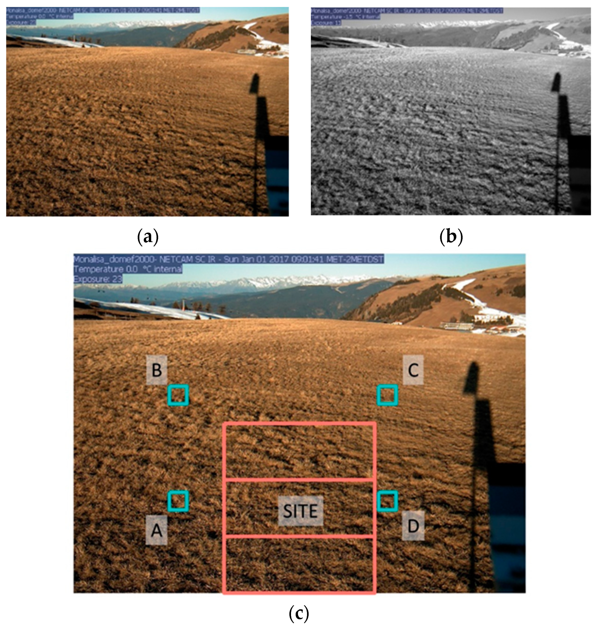
The Phenocam sensor we used is a Hybrid IP StarDot 1.3 Megapixel Netcam SC, Model SD130BN (StarDot Technologies, Buena Park, CA, USA). Acquisitions have been automatically made every 30 min during periods with daylight since 2015. Both an RGB image (Figure 4a) and a monochrome combination of RGB + Near Infrared (Figure 4b) are taken a few seconds apart with dynamic exposure times. A removable Infrared (IR) filter is applied to a Complementary Metal-Oxide Semiconductor (CMOS) sensor enabling the removal of the IR signal for the RGB image [57] dissolved into three bands. About 2 m above each MONALISA station, a Phenocam is installed facing north towards the grassland site. In 2017, each of the Phenocams collected between 4283 (Domef1500) and 4681 (Vimef200) usable pairs of images in RGB and RGB + NIR bands depending on the network status and the file corruption during transfer. In addition, in July 2017, the transmission of the Phenocam of the Vimes1500 station had a problem with the transfer, causing a period of 14 days without acquisition. The spectral bands have the highest spectral response around 450 nm (B), 530 nm (G), and 600 nm (R) [19]. The red band integrates over a wide range of wavelengths, capturing parts of the near infrared spectrum [20]. The NIR band range is not documented, but the quantum efficiency of CMOS sensors at normal operation temperatures drops to zero in the range of 1050–1100 nm due to the low photon energy. The calculation of the NDVI index from the Phenocams adheres to the approach suggested by Petach et al. [26].
The RGB image (YDN) is analyzed by its single digital numbers (DN) in each band (RDN, GDN, and BDN) (Equation (2)). The digital number in the RGB+IR image (ZDN) is considered as a sum of YDN and an infrared component (XDN) (Equation (3)).
In the case of the Stardot Phenocam, the values have to be corrected by the exposure of the RGB+IR image (EZ) and RGB image (EY) in order to retrieve the exposure corrected NIR value (X′DN, Equation (4)) as well as the red value (R’DN, Equation (5)) for NDVI calculation (Equation (6)):
For the setup of the working environment, the Phenopix R-package was used [25]. The exposure times needed for the NDVI computation are stored as text directly on the image. We extracted the value using several statistical approaches, such as clustering and brightness as well as the Tesseract OCR [58]. A visual validation of approximately 1200 pairs of images across sites indicated an exposure retrieval rate of 100%.
Besides exposure and acquisition times, the NDVI values can be influenced by several sources of error, such as corrupted images, precipitation, water or snow-covered lens, fog, cloud, and cloud or topographic shadows as well as livestock or human activities. Such errors can occur abruptly within one image or, more probable, for more consequently recorded images. In order to reduce these influences, we excluded pictures with exposure times longer than 50 s as well as exposure ratios (RGB/IR) lower than 2 [26] and acquisition times earlier than 10 am, respectively, later than 4 pm. In order to represent the NDVI from the single Plots A, B, C, and D (Figure 2), we applied multiple Regions of Interests (ROI) to the images. The four ROIs cover 25 × 25 pixel each and represent the four plots (Figure 4c) on each site. The three bigger ROIs in the middle of the picture represent the whole site plot. The Phenocam NDVI values are generated in a four-step filtering process: (i) Within an image, (ii) within a day, (iii) within a moving window of 4 days, and (iv) the resulting 90% percentile of NDVI values [19,26,59]. First, the ROIs are analyzed by their heterogeneity (mean, standard deviation) and divergent ROIs are excluded. The resulting NDVI values are filtered within a day and a moving window of four days by computing the density of the daily NDVI. We applied the standard deviation (filtering of lower values) together with the 2*interquartile range (IQR, filtering for extremely high values). The final NDVI values are determined by the 90% percentile of the values per day. This allowed us to reduce noise, but also to avoid the exclusion of brief dynamic changes within the NDVI signal. Since this study aims at evaluating each sensor individually, we did not calibrate the Phenocam NDVI values with ancillary optical data sources to avoid issues related to sun illumination and reference material deterioration [19,26,59].
2.4.3. Spectral Reflectance Sensor (SRS)
Each of the stations is equipped with an SRS sensor produced by Decagon (METER Group Inc., Pullman, WA, USA) continuously measuring the NDVI since 2015. The bands are centered at 650 nm (Red) and 810 nm (NIR) with a full-width half-max of 10 nm. The SRS sensor for measuring the NDVI signal is composed of two different versions: One hemispherical version (Ni) facing upwards and collecting the incoming radiation and a field stop version (Nr) aligned to the grassland at approximately a 30° inclination angle [60]. The SRS sensors are oriented towards the north, in the same direction as the Phenocam. In the case of the Vimes1500, the SRS sensor is pointed more towards the east. This was necessary since the Phenocam is oriented towards an enclosed part of the meadow not managed by the farmer. The MONALISA stations have been installed at the boundaries of the grassland sites. The inclination angle allows recording of the NDVI signal of the grassland within the managed grassland sites, reducing edge effects. SRS sensors are mounted at approximately a 1.8 m height. Downwards facing sensors have an FOV of 36°, covering a total ground area of approximately 1 m2 in our setup. The measurement frequency is every 15 min and the measurements are automatically transmitted by the station to a central receiver and transmitted to the publicly exposed MONALISA Database (http://monalisasos.eurac.edu/sos/) based on the Open Geospatial Consortium (OGC) Sensor Observation Service (SOS) v2.0 standards [23,61]. The SRS data has been filtered similarly as the Phenocam images by applying the standard deviation and IQR to the density of the distribution for removing outliers. This procedure helps to minimize the influence of periods with changing weather conditions (e.g., rain, cloud coverage) since they cannot be visually identified as in the Phenocam images.
2.4.4. Spectroradiometer
The hyperspectral spectroradiometer used for the collection of in-situ measurements was an SVC HR-1024i (Spectra Vista Corporation, New York, NY, USA) with 1048 spectral bands ranging from 338 nm to 2500 nm. The spectral wavelengths relevant for computing the NDVI were recorded with a Silicon array measuring in 512 spectral bands and a spectral resolution of ≤3.5 nm FWHM from approximately 338 to 1000 nm [62]. We conducted in total 26 field campaigns (2 in Vimef2000, 12 in Vimes1500, 5 in Domef1500, 7 in Domef2000) from May to October 2017. The differences were due to unstable or bad weather conditions during the field campaigns. The spectrometer was mounted at an altitude of approximately 1.2 m above ground pointing nadir at the grassland. We collected the measurements in a time range between 10:00 and 14:00 MEST depending on the number of sites and weather conditions during the days. The standard foreoptic lens mounted on the spectroradiometer had a 4° FOV, allowing the integration of an area covering approximately 50 cm2. Before each measurement, we took a reference measurement on a white reflectance panel (Spectralon), an automated dark measurement, and we set the integration time to 5 ms. This integration time was suitable for typical illumination conditions. The measurements at Domef1500, Domef2000, and Vimef2000 sites were conducted until the first harvest event. The measurements on the Vimes1500 site continued until the end of the growing season in October. We took three to four spectrometer measurements for each of the four 50 cm2 plots to reduce sources of error/uncertainty, such as shadows or open soil, and to quantify the whole plot measured, resulting in a mean NDVI for each plot, totaling in 421 spectroradiometer measurements across sites. The high spectral resolution of the spectroradiometer allowed NDVI computation integrating different wavelengths. For determining the optimal band combination for the NDVI, we evaluated different red and NIR band ranges varying from those of SRS (648–652 Red and 808–812 NIR) to the Sentinel-2 MSI (635–695 Red and 727–957 NIR). We found a correlation of R2 > 0.95 for the NDVIs generated. Since the SRS wavelengths are present in each of the instruments, we decided to generate the spectroradiometer NDVI based on the bandwidths of the SRS sensor.
2.5. NDVI Signal Comparison
We compared the NDVI time series of different sensors and analyzed them with regard to different attributes as well as spatial scales. We aimed at evidencing similarities, differences, sensor-specific characteristics, errors, or problems resulting from the NDVI signal acquired by different sensors on diverse scales for monitoring grassland sites during the year. We especially focused on the different properties of the grassland sites, such as altitude, management, exposure, and location as well as the characteristics of the sensors. This was done, as can be seen in Figure 2, once for the sensor-specific spectral signatures of the whole site (Section 3.1) as well as for the four plots of each site (Section 3.2).
We utilized simple statistics, such as the mean and standard deviation, to describe the spectral signatures and later computed linear regression to determine the signal similarity over time. For analyzing the performance of the regression, we used the linear correlation coefficient (R), the coefficient of correlation (R2), and the p-value. We utilized the R in order to see the positive and negative correlations between two values, especially for the autocorrelation measurements as implemented in the R package “forecast” [63]. The R2 is a widely used correlation coefficient for calculating the ratio between the total and the explained variation by the model (Equation (7)) [52,64]:
where represents the observations, R their residuals, and y* the mean of . The p-value is used to determine the grade of significance for the conducted correlation analyses and is mainly applied for understanding the reliability of the correlation between the sensors. Additionally, we studied whether the temporal resolution or the spectral response of the sensor causes time lags of the NDVI signal correlation by calculating the cross-correlation between the NDVI values of sensors. The detectability of short-term changes was addressed by visually extracting harvesting and snow events from each of the Phenocams. We first visually interpreted the relation between the NDVI signals and the dynamic events before analyzing the spatial differences among the plots on each site depending on a sensor and in relation to an event.
3. Results
3.1. Optical Responses by Site
The optical responses of the NDVIs across the sites are shown in Figure 5 together with brief events of snow and harvesting. On all four sites, the NDVI shows a similar behavior over time clearly following the vegetation growth during the year with an increase of the NDVI signal in spring and a decrease towards the end of the year. Despite showing similar curves, the NDVI signals show a different range. Sentinel-2 and Spectrometer NDVI range between 0.23 and 0.93 and between 0.65 and 0.92, whereas the SRS NDVI ranges are much lower (−0.19 and 0.827). Phenocam NDVI values are lowest and never surpassed a value of 0.55 and even show negative values down to −0.57 before the start of vegetation growth and after harvesting events.
The NDVI signal encompassing snow periods reacts differently among sensors. During snow-periods, the temporal resolution of Sentinel-2 and the high cloud coverage impedes a detailed study of the events whereas the other sensors constantly, but restrictively, detect the spectral signal. The SRS responds with an inferior (Vimes1500) or noisier (Domef2000, Vimef2000) NDVI signal. The Domef1500 site shows no clear differences during snow events except an elevated NDVI value during the first snow period at the beginning of March and the last snow period in May, probably due to erroneous acquisitions overestimating the NDVI. The Phenocam NDVI shows no clear trend during snow phases except a higher noise in the NDVI signal. Harvesting periods are best represented in the Domef1500 signals of all sensors by an abrupt decline of the NDVI signal and a local minimum of two to three days after the event. It is similar on the Vimes1500 site although Phenocam and Spectrometer do not reflect changes in NDVI at the first harvest due to the 14 day lasting failure of the Phenocam and the 10 day delay of the spectrometer measurement. On the sites at the 2000 m height, the harvests are less detectable than at 1500 m. For the Domef2000 site, we see a decline in the NDVI value just for Sentinel-2 and, less intensively, for Phenocam. The SRS shows no response. The numerous harvesting periods occurring on the Vimef2000 site are difficult to detect, especially on the level of Sentinel-2 having a detection gap from the beginning of July to August. SRS detects only the first and last harvesting and the Phenocam NDVI signal lowers after the first cut. The most evident change in NDVI signal for both sites on 1500 m happened within seven days after a harvesting event before quickly recovering with an increasing plant canopy density. On both 2000 m sites, response and recovery are less evident and are similar for each instrument.
The linear correlations among sensors per each site are listed in Table 2 (right column). We used the linearly interpolated time series for each sensor and correlated the data from time periods both sensors acquired to have same day acquisitions to compare. The best correlations result was comparing Phenocam NDVI to SRS NDVI (R2 between 0.82 and 0.87) and to Sentinel-2 NDVI (R2 between 0.67 and 0.76) as well as between SRS NDVI and Sentinel-2 NDVI (R2 between 0.74 and 0.82). The R2 of the spectrometer NDVI to the others differs significantly among all sensors ranging from 0.07 to 0.88. The exceptionally high correlation between the spectrometer and Sentinel-2 sensors on the site, Vimef2000, is due to the least amount of samples and the linear interpolation. The Vimes1500 station, continuously monitored during the growing phase, shows a steady, but low correlation from 0.4 to 0.53 possibly due to the 14-days Phenocam blackout, the different viewing angles of SRS and Phenocam, or the steepness of the site.
The results from the NDVI cross-correlation analysis between the sensors of Phenocam, Sentinel-2 MSI, and SRS are shown in Figure 6. The spectrometer NDVI is not taken into consideration due to its limited number of samples over time. Cross-correlation shows that a lag of around 0 days leads to the highest correlations between Phenocam and SRS. Comparing the Sentinel-2 imagery to SRS and Phenocam, the curve tends to have the highest correlation with a lag of 0 to −2 days, probably due to the temporal resolution of the Sentinel-2 imagery. The cross-correlation between Phenocam and Sentinel-2 MSI for Vimes1500 shows a maximum correlation with a lag from −5 to −10 days, but has a limited validity due to the low correlation coefficient (R < 0.5). Overall, the correlation coefficients in time vary in dependence of the altitudes of 1500 m and 2000 m, which is most probably caused by the considerably higher spectral response during growth and harvesting events (see Figure 5). The cross-correlations between Phenocam and SRS as well as SRS and Sentinel-2 MSI on 2000 m tend to be asymmetric with a similar and elevated R, a further indication of less variation in the original spectral signature on the 2000 m sites.
3.2. Optical Responses by Plot
The NDVI signals for each of the four plots A, B, C, and D are shown in Figure 7 and delimited by each of the four meadow sites in 2017. Analyzing the plot with multiple measurements allows estimation of the difference of an NDVI signal for each of the sites.
The linear correlation for each plot (A, B, C, and D) and the corresponding sensors is shown in Table 2. It shows the number of NDVI values, the combination of R2, and the level of significance. No SRS NDVI measurements are available for the plots. Although lying within the same site, the linear correlation among plots differs depending on the site and sensor. The Domef1500 site shows a good correlation between the NDVIs of Phenocam and Sentinel Sensors (0.67 < R2 < 0.8) of each plot. As for the site, the spectrometer has low R2 with all the sensors (0.03 < R2 < 0.54) on each plot, again caused by the saturation effect occurring in all the spectrometer measurements as well as by the low amount of spectrometer measurements. The Domef2000 site R2 is similar to Domef1500, with high correlations between Sentinel-2 MSI and Phenocams (0.60 < R2 < 0.80). At the same time, the Spectrometer NDVI shows an equally low correlation with the Sentinel-2 MSI and Phenocams (0.00 < R2 < 0.72). The Vimef2000 site shows the highest correlations among all sensors and plots especially between the spectrometer and Phenocam (0.78 < R2 < 0.82). As for the site analysis of the Vimef2000, the R2 between the spectrometer and the other sensors cannot be analyzed due to the limited availability of spectrometer measurements. The correlations between the Phenocam and Sentinel-2 are slightly higher than for the Domef sites (0.74 < R2 < 0.77). The Vimes1500 site has the lowest R2 between Phenocam and Sentinel 2 (0.12 < R2 < 0.31), but the longer time series of the spectrometer causes a more stable although low correlation between Spectrometer and Phenocam (0.39 < R2 < 0.52) as well as the Spectrometer and Sentinel-2 (0.44 < R2 < 0.58). Comparing the plot to the site correlation, we see that in most cases, they have a similar trend across scales even though differences of up to 0.2 are visible in some cases.
Similar to the complete sites, the vegetation period can also be seen on the plot level by each of the sensors NDVI. The linearly interpolated time series of the Sentinel-2 MSI sensor shows little change among the four plots, i.e., among the four neighboring pixels. The mean standard deviation of the acquisitions lies between 0.012 (Domef1500) and 0.017 (Domef2000). The Phenocam has the highest mean standard deviation between measurements of 0.228 (Vimes1500) and 0.0504 (Domef2000). Regarding all sensors, the Vimes1500 station has the minimum mean standard deviation of 0.265 whereas the Domef2000 station has the highest differences between the measurements of all scales (0.471). Throughout the stations, the mean standard deviations for each sensor can be considered very low. Nevertheless, in some parts of the NDVI signature, we see differences in the NDVI response. The Domef1500 site shows different NDVI changes during the first snow events at the end of May. The Phenocam NDVI signature of Plot A shows a greater decline than the other three plots. On the Domef2000 site, we see differences in the NDVI values per plot calculated from the spectrometer. Especially, the second acquisition on 31st May shows variable NDVI values ranging from 0.631 to 0.847. At the same time, the Phenocam plots within the station show differences when evaluating the cut event. Vimef2000 shows notable differences in the NDVI signal acquired from the Phenocams during the first harvest. This is caused by the different harvesting intervals on the Vimef2000 site affecting only some of the ROIs.
Figure 8 shows that the NDVI variation within a plot in most cases lies between 0 and 0.1 among sensors for each site showing stable NDVI results per measurement day. For short-term changing events of snow and especially harvesting events, the NDVI variation for each plot reaches higher values of 0.1 to 0.23 (Domef1500 harvest). This result suggests that a denser canopy shows higher spectral variability within the site than expected when sensor saturation is reached after the growth phase. The Vimef2000 NDVI signal shows a local peak around the harvest in August 2017 and the Vimes1500 station during the first snow event in May 2017, but not during harvesting. These trends from Phenocams are less obvious for both the other two scales although the Sentinel-2 NDVI varies mostly around the harvesting period of Vimef2000 and Vimes1500 and during the first snow event at Domef1500. The spectrometer measurements show a higher variability of the signal during the second harvest event for the Vimes1500 site.
4. Discussion
The presented study shows that the acquired NDVI signals diverge considerably depending on the sensor being utilized. These are likely due to the specific acquisition conditions of the sensors, namely the spatial scale of detection, the temporal resolution, or detection geometry.
4.1. Sensor Specifications and Geometry
Unlike the other sensors, the spectrometer NDVI is difficult to interpret in terms of vegetation dynamics since the generation of a meaningful time series requires stable illumination, i.e., weather condition, good accessibility of the plot, workforce, and time for preparation and analysis. Especially on higher altitudes, the number of possible spectrometer measurements is limited in time and space during one single year. In 2017, the growth phase of vegetation was affected by bad weather and late snow in April/May. Therefore, we were not able to conduct appropriate field measurements over this period. Additionally, the weather conditions on the Vimef2000 site were often variable during the field campaigns, resulting in fewer acquisitions. The restrictions for collecting spectrometer measurements make it difficult to integrate them into a combined sensor approach other than as reference or calibration for other sensors [35,36]. Spectrometer measurements have been found to correlate best with the Sentinel-2 NDVI signal, most probably because they both measure under near-nadir circumstances and tend to saturate quickly. Considering the most reliable time series measured on the Vimes1500 site, we are not able to visually extract a connection to the first harvesting event due to a delay of 10 days after the harvest resulting in a slightly higher NDVI signal than before the harvest, indicating a full recovery of the plant canopy. The signal before and after the second harvest leaves a clearer mark despite the time gap of roughly one month. For spectrometer NDVI on alpine grassland sites, measurements of one week before and after a harvesting event are crucial. Measurements taken afterwards possibly miss the events due to the quick recovery of the plant canopy density.
The SRS sensor provides the most stable NDVI curves among all sensors. The exclusion of extreme values and time ranges at the beginning and the end of the day, as well as the implementation of a threshold filtering for the 90% percentile for the NDVI signal, results in a steady signature. However, the NDVI signal continuously underestimates the NDVI compared to the spectrometer and Sentinel-2 MSI NDVIs by 0.1 to 0.3, which is most likely due to its 30° inclination angle or due to issues with the calibration of the sensor. Additionally, the SRS sensor renders no information about error sources (e.g., changing light conditions, snow, precipitation, water presence, or human interaction) and is not extensively usable, returning only one single NDVI information of a plot near the station. Collecting NDVI with an SRS sensor mounted on an environmental station, as presented in this study, forces it to detect only marginal parts of the grassland. It could be useful to integrate multiple sensors pointed at different locations of the grassland or to manage the same sensors manually, e.g., during field campaigns, to quantify the NDVI differences between the measured plot and the overall site. Especially when compared to sensors measuring more extensively (e.g., Sentinel-2 MSI and Phenocam) on sites with inconstant and multiple management activities, the SRS NDVI signatures can prove to be inconsistent. This explains the difficulties of recording harvest events on the sites. The plots on 1500 m a.s.l show a better signal response than the plots on 2000 m a.s.l., which is probably due to the complete harvesting of the whole meadow within one day. On the other hand, the signal response shortly before and after snow events varies from slightly higher to considerably lower and noisy NDVI signatures. Here, the snowmelt process and the light conditions could influence the sensor since the snow melts at different rates throughout the day. The high temporal resolution within a day could be interesting for further expanding this analysis on the detection of the snow patchiness on grasslands.
The NDVI signal derived from Phenocam imagery is difficult to standardize and filter. The band range and the mechanical IR filter properties are not clearly defined and documented in the literature. Additionally, the viewing/inclination angle of the Phenocams is probably the source for underestimation of the NDVI signal. Despite these limiting factors, the correlations retrieved between the Phenocams, Sentinel-2, and SRS are very promising. The NDVI signal seems to be very robust through time over the sites of Domef1500, Domef2000, and Vimef2000 [19]. The only site with less correlation is Vimes1500. The weaker correlation could result from the diverging positioning of the SRS sensor with respect to the Phenocam, the south exposure, or the Phenocam failure shortly after the first harvest period. The approach used for calculating Phenocam NDVI is considered to be an estimate and can be scaled either by spectrometer [26] or by satellite-based NDVI values [19]. Results suggest that Phenocam NDVI is underestimated continuously, but differently depending on the site and growing phase. Other than the NDVI, the Green Chromatic Composite (GCC, [19,65]) or the Excess Green Index (EXG, [66,67]) discount the RGB+IR image have been widely researched and are considered to relate to phenological stages in grasslands [59].
Monitoring grasslands with remote sensing methods mostly lacks a standardized approach for integrating multiple sensors [6]. Sentinel-2 MSI imagery, with the advantages in temporal availability and spatial resolution, showed that both the annual [68] growing phases, as well as dynamic short-term changes within grasslands, are well representable. Sentinel-2 images on Vimes1500 are less constant than for the other three sites, which is most probably due to the influence of the slope and aspect of the site. An additional topographic correction could be very helpful to correct the images in a proper manner although it is difficult to be adequately geolocated in heterogeneous mountainous areas. As weather, or cloudiness, is the crucial constraint of optical Sentinel-2 data, the combination with other remote sensing data, such as Landsat 8, may lead to a slightly better time series [32,34,69]. However, the combination of remote sensing imagery with other optical sensors, such as Phenocams and SRS, provides reliable information on the slightest changes of the spectral signal each day and makes it easier to monitor the dynamics in grassland communities. At the same time, the NDVI acquired with Phenocam and especially SRS tend to be stable under inconsistent weather conditions, such as clouds or shadows, which is most probably due to the number of measurements and the possibility to reduce noise by filtering and the availability of images during cloudy periods. Therefore, both sensors are equally useful when creating a combined sensor workflow. By analyzing the meadows on a subplot level, we noticed considerable differences within the NDVI signals of one plot (up to 0.2). This may result in the time lag hampering a simultaneous acquisition on each scale, the linear filtering of the NDVI values, or heterogeneity within vegetation of the study sites. We found that sensors detecting the ground in a near-nadir position (Sentinel-2, Spectroradiometer) have higher overall NDVI values than SRS installed at a 30° inclination as well as the very variable inclination of the Phenocams recording the lowest NDVI values. This indicates that the viewing geometry of the optical sensors constantly influences the NDVI signal over time, resulting in an underestimation of the NDVI [70,71].
4.2. Temporal and Spectral Resolution
The temporal scale of acquisition influences the detection of short-term events. In the case of both meadows on 1500 m a.s.l., the NDVI signal experiences the highest change within the 2 weeks after the event, but is not always applicable to each of the events (e.g., the second harvest on Vimef1500) for the Sentinel-2 MSI image. Within the sites on 2000 m a.s.l., the temporal gaps in Sentinel-2 imagery made it difficult to determine the exact harvest event when multiple harvests took place during the year. For the detection of snow events, the weather conditions during the measurement must be stable. Especially for Sentinel-2 imagery, a snow event lowers the availability of images augmenting the usefulness of alternative sensors, such as SRS or Phenocam. Later snow events are particularly difficult to characterize by remote-sensing images due to a rapid snowmelt process caused by the elevated temperatures later in the year. Especially Phenocams in combination with SRS sensors have the appropriate temporal characteristics to assess snowmelt and snow patches on grassland sites [49].
The spectral resolution of the instruments limited the research, arguably due to the lack of computable and comparable VIs from each sensor as well as the diverse or poorly documented length of the Phenocam spectral bands. The SRS is able to reproduce only NDVI and PRI indices. Phenocams can be used for generating more VIs, such as GCC or EXG, but are less accurate when it comes to combining both images (RGB and RGB+IR) in one single index (e.g., NDVI). On the other hand, Sentinel-2 is able to create a wide variety of indices and the spectral resolution of the spectrometer allows the creations of most of the vegetation indices aside the ones requiring thermal information.
4.3. Potential for Combined Sensor Appoach
The results of the analyses demonstrate that the NDVI signals have a high correlation among each other, favoring their combination in a multisensor approach. In general, the signal acquired from diverse sensors are comparable and offer the opportunity to fill data gaps or as a source of calibration among each other. Despite the elevated Sentinel-2 MSI, Phenocam, and SRS correlation among time series during the year, the detection of crucial phases or short-term changes in vegetation growth, offset in the NDVI signal or differences in their signal saturation, are strongly sensor and site dependent [46]. The analysis shows that the short-term dynamic changes of the vegetation are not equally represented by the optical sensors of choice, differing by management practice, extent and date, revisit frequency, or time gaps. Grassland sites with clear cutting events, such as Vimes1500 and Domef1500, are represented equally well by Sentinel-2 MSI, SRS, and Phenocam (aside the first cut on Vimes1500). The sites on 2000 m a.s.l.—being diverse in their vegetation growth, grassland composition, and management activities—show, however, that one single sensor lacks the capability to evidence all changes. Examples are the detectability of the cutting event on Domef2000 as well as the unstable detectability of the multiple harvesting events on the Vimef2000 site. The detection of snow has proven to be difficult for Sentinel-2 MSI, SRS, and Phenocam sensors. This result was from a lack of images or the inconsistent signal measured by the sensors during phases of snowfall and snow acquisition. Despite clear signal changes being visible, they do not tend to minor (as we would have expected) or elevated NDVI values, but signal an incoherent NDVI value. A common property is that each NDVI signal during and after a snow event suffers a period of less NDVI signal growth (e.g., snow period at the beginning of May on the Domef1500 site). Nevertheless, this is not equally representable throughout the stations since the grassland vegetation onset is diverse on 1500 and 2000 m a.s.l. as well as snow amount and frequency divergences depending on the site. This indicates that a multisensor approach for monitoring mountainous grassland vegetation must address the specific regions of interest as well as their topographic properties and management activities. It should also include the possibility to compute different indices, such as the NDSI, better suited when analyzing or masking the presence of snow periods.
The calibration of the sensor specific signal has to be addressed as one of the most pressing issues when considering a multisensor approach. The comparison of the spectral signatures requires a dedicated a-priori calibration, especially for Phenocam imagery, whose spectral properties make a computation of the NDVI index less comparable to the other sensors. A simple correction of one sensor integrating the spectral signal of another is considered insufficient. Especially, short-term changes are not represented equally throughout the sensors. The combination of NDVIs from the sensors would result in either a lack of knowledge of short-term changes or an erroneous correction of one signal. Examples are the first snow period in Domef1500, the first harvest in Vimes1500, or the single cutting events in Vimef2000. Additionally, the inconsistent increase of the NDVI becomes evident during the growth period on Domef2000 (SRS, Phenocam) or the period between the harvests on Domef2000 (S2 vs. Phenocam or SRS).
5. Conclusions
This study renders a detailed overview of the behavior of the NDVI acquired by different sensors over diverse spatiotemporal scales. Even though SRS, Phenocams, and Sentinel-2 MSI were able to trace the vegetation growth in a similar manner, we conclude that the same index can have notable differences both within a grassland site and among sensors depending on spatial and temporal resolution and heterogeneity of the targeted grassland. We demonstrated sensor-specific NDVI signal offset as well as different increases in NDVI signals during the growing period in spring. Simultaneously, short-term dynamic changes were represented differently by the sensors in terms of NDVI intensity changes, the management process, and extensiveness as well as the site location (especially concerning the altitude). We demonstrated that the combination of the NDVI by multiple sensors enhanced the possibility for detecting short-term dynamic changes throughout the year for each of the stations.
In the future, it seems promising to unify the spectral response acquired on multiple scales within a standardized workflow, enhancing the characterization of grassland dynamics within mountainous regions. Standardization efforts as formulated by the OGC are useful to collect, sort, store, access, and process data from different sensors in a unified way. Furthermore, the inclusion of other biophysical parameters (e.g., LAI or fAPAR) derived from optical sensors and biophysical models could lead to an augmented detectability of dynamic changes of grassland and enable the assessment of its status, stress levels, phenological stages, or biomass increase throughout the year. At the same time, the synergetic use of other optical sensors or microwave remote sensing indicates great potential in future vegetation analyses, reducing spatial uncertainties or temporal gaps that occur individually among sensors. Especially for mountainous vegetation, factors, such as elevation, topography, sun geometry, or the presence of clouds as well as cloud shadows, impact the optical response of grasslands. Therefore, it is advisable to include corrections of the inclination angle or the correction of topographic effects, such as BRDF, for the analysis of alpine vegetation as well as detailed detection of cloud, cloud shadow, and haze.
Author Contributions
Conceptualization, M.R., S.A., G.N., M.Z., G.T.; Methodology, M.R.; Data Curation and Software Development, M.R.; Field Work and Data Collection, M.R.; Writing—Original Draft Preparation, M.R.; Writing—Review and Editing, S.A., G.N., M.Z., E.T., G.T.; Supervision, S.A., G.N., M.Z., G.T.
Funding
This research was funded the Free University of Bolzano in collaboration with Eurac Research. The authors thank the Department of Innovation, Research and University of the Autonomous Province of Bozen/Bolzano for covering the APC costs.
Acknowledgments
The authors want to acknowledge the infrastructure constructed within the MONALISA project funded by the Autonomous Province of South Tyrol. Additionally, the authors would like to thank Jeroen Staab for providing help in processing of the Phenocam images and SRS sensors as well as Abraham Mejia Aguilar and Johannes Klotz for their support during field campaigns and advice on the instruments utilized in this study. Moreover, the authors would like to acknowledge Karin Steinberger and Teresa Beever from Übersetzungsbüro Steinberger for reviewing the English language.
Conflicts of Interest
The authors declare no conflict of interest.
References
- White, R.P.; Murray, S.; Rohweder, M. Pilot Analysis of Global Ecosystems: Grassland Ecosystems; World Resources Institute: Washington, DC, USA, 2000. [Google Scholar]
- Ali, I.; Cawkwell, F.; Dwyer, E.; Barrett, B.; Green, S. Satellite remote sensing of grasslands: From observation to management. J. Plant Ecol. 2016, 9, 649–671. [Google Scholar] [CrossRef]
- European Economic Area (EEA). CLC Addendum to CLC2006 Technical Guidelines—Final Draft. Available online: https://land.copernicus.eu/user-corner/technical-library/Addendum_finaldraft_v2_August_2014.pdf (accessed on 29 January 2019).
- French, K.E.; Tkacz, A.; Turnbull, L.A. Conversion of grassland to arable decreases microbial diversity and alters community composition. Appl. Soil Ecol. 2017, 110, 43–52. [Google Scholar] [CrossRef]
- Lüth, C.; Tasser, E.; Niedrist, G.; Via, J.D.; Tappeiner, U. Plant communities of mountain grasslands in a broad cross-section of the Eastern Alps. Flora 2011, 206, 433–443. [Google Scholar] [CrossRef]
- Xu, D.; Guo, X. Some insights on grassland health assessment based on remote sensing. Sensors 2015, 15, 3070–3089. [Google Scholar] [CrossRef] [PubMed]
- Ali, I.; Greifeneder, F.; Stamenkovic, J.; Neumann, M.; Notarnicola, C. Review of Machine Learning Approaches for Biomass and Soil Moisture Retrievals from Remote Sensing Data. Remote Sens. 2015, 7, 16398–16421. [Google Scholar] [CrossRef]
- Jankowska-Huflejt, H. The function of permanent grasslands in water resources protection. J. Water Land Dev. 2006, 10, 233. [Google Scholar] [CrossRef]
- Theurillat, J.P.; Guisan, A. Potential Impact of Climate Change on Vegetation in the European Alps: A Review. Clim. Chang. 2001, 50, 77–109. [Google Scholar] [CrossRef]
- Della Chiesa, S.; Bertoldi, G.; Niedrist, G.; Obojes, N.; Endrizzi, S.; Albertson, J.D.; Wohlfahrt, G.; Hörtnagl, L.; Tappeiner, U. Modelling changes in grassland hydrological cycling along an elevational gradient in the Alps. Ecohydrology 2014, 7, 1453–1473. [Google Scholar] [CrossRef]
- Niedrist, G.; Tasser, E.; Bertoldi, G.; Della Chiesa, S.; Obojes, N.; Egarter-Vigl, L.; Tappeiner, U. Down to future: Transplanted mountain meadows react with increasing phytomass or shifting species composition. Flora 2016, 224, 172–182. [Google Scholar] [CrossRef]
- Gitelson, A.A.; Merzlyak, M.N.; Lichtenthaler, H.K. Detection of Red Edge Position and Chlorophyll Content by Reflectance Measurements near 700 nm. J. Plant Physiol. 1996, 148, 501–508. [Google Scholar] [CrossRef]
- Horler, D.N.H.; Dockray, M.; Barber, J. The red edge of plant leaf reflectance. Int. J. Remote Sens. 1983, 4, 273–288. [Google Scholar] [CrossRef]
- Rouse, J.W.; Haas, R.H.; Schell, J.A.; Deering, D.W. Monitoring Vegetation Systems in the Great Plains with ERTS. In Proceedings of the 3rd ERTS Symposium, Washington, DC, USA, 10–14 December 1973; pp. 309–317. [Google Scholar]
- Browning, D.; Karl, J.; Morin, D.; Richardson, A.; Tweedie, C. Phenocams Bridge the Gap between Field and Satellite Observations in an Arid Grassland Ecosystem. Remote Sens. 2017, 9, 1071. [Google Scholar] [CrossRef]
- Enciso, J.; Maeda, M.; Landivar, J.; Jung, J.; Chang, A. A ground based platform for high throughput phenotyping. Comput. Electron. Agric. 2017, 141, 286–291. [Google Scholar] [CrossRef]
- Gamon, J.A.; Kovalchuck, O.; Wong, C.Y.S.; Harris, A.; Garrity, S.R. Monitoring seasonal and diurnal changes in photosynthetic pigments with automated PRI and NDVI sensors. Biogeosciences 2015, 12, 4149–4159. [Google Scholar] [CrossRef]
- Richardson, A.D.; Braswell, B.H.; Hollinger, D.Y.; Jenkins, J.P.; Ollinger, S.V. Near-surface remote sensing of spatial and temporal variation in canopy phenology. Ecol. Appl. 2009, 19, 1417–1428. [Google Scholar] [CrossRef] [PubMed]
- Filippa, G.; Cremonese, E.; Migliavacca, M.; Galvagno, M.; Sonnentag, O.; Humphreys, E.; Hufkens, K.; Ryu, Y.; Verfaillie, J.; Di Morra Cella, U.; et al. NDVI derived from near-infrared-enabled digital cameras: Applicability across different plant functional types. Agric. For. Meteorol. 2018, 249, 275–285. [Google Scholar] [CrossRef]
- Brown, T.B.; Hultine, K.R.; Steltzer, H.; Denny, E.G.; Denslow, M.W.; Granados, J.; Henderson, S.; Moore, D.; Nagai, S.; SanClements, M.; et al. Using phenocams to monitor our changing Earth: Toward a global phenocam network. Front. Ecol. Environ. 2016, 14, 84–93. [Google Scholar] [CrossRef]
- Srbinovska, M.; Gavrovski, C.; Dimcev, V.; Krkoleva, A.; Borozan, V. Environmental parameters monitoring in precision agriculture using wireless sensor networks. J. Clean. Prod. 2015, 88, 297–307. [Google Scholar] [CrossRef]
- Aqeel-ur-Rehman; Abbasi, A.Z.; Islam, N.; Shaikh, Z.A. A review of wireless sensors and networks’ applications in agriculture. Comput. Stand. Interfaces 2014, 36, 263–270. [Google Scholar] [CrossRef]
- Reed, C.; Botts, M.; Davidson, J.; Percivall, G. Ogc® sensor web enablement: Overview and high level achhitecture. In Proceedings of the 2007 IEEE Autotestcon, Baltimore, MD, USA, 10–20 September 2007; pp. 372–380. [Google Scholar]
- Kulmala, M. Build a Global Earth observatory. Nature 2018, 553, 21–23. [Google Scholar] [CrossRef]
- Filippa, G.; Cremonese, E.; Migliavacca, M.; Galvagno, M.; Forkel, M.; Wingate, L.; Tomelleri, E.; Di Morra Cella, U.; Richardson, A.D. Phenopix: A R package for image-based vegetation phenology. Agric. For. Meteorol. 2016, 220, 141–150. [Google Scholar] [CrossRef]
- Petach, A.R.; Toomey, M.; Aubrecht, D.M.; Richardson, A.D. Monitoring vegetation phenology using an infrared-enabled security camera. Agric. For. Meteorol. 2014, 195–196, 143–151. [Google Scholar] [CrossRef]
- Cremonese, E.; Filippa, G.; Galvagno, M.; Siniscalco, C.; Oddi, L.; Di Morra Cella, U.; Migliavacca, M. Heat wave hinders green wave—The impact of climate extreme on the phenology of a mountain grassland. Agric. For. Meteorol. 2017, 247, 320–330. [Google Scholar] [CrossRef]
- Richardson, A.D.; Hufkens, K.; Milliman, T.; Aubrecht, D.M.; Chen, M.; Gray, J.M.; Johnston, M.R.; Keenan, T.F.; Klosterman, S.T.; Kosmala, M.; et al. Tracking vegetation phenology across diverse North American biomes using PhenoCam imagery. Sci. Data 2018, 5, 1–24. [Google Scholar] [CrossRef] [PubMed]
- Loveland, T.R.; Irons, J.R. Landsat 8—The plans, the reality, and the legacy. Remote Sens. Environ. 2016, 185, 1–6. [Google Scholar] [CrossRef]
- Deilami, K.; Hashim, M. Very High Resolution Optical Satellites for DEM Generation: A Review. Eur. J. Sci. Res. 2011, 49, 542–554. [Google Scholar]
- Malenovský, Z.; Rott, H.; Cihlar, J.; Schaepman, M.E.; García-Santos, G.; Fernandes, R.; Berger, M. Sentinels for science: Potential of Sentinel-1, -2, and -3 missions for scientific observations of ocean, cryosphere, and land. Remote Sens. Environ. 2012, 120, 91–101. [Google Scholar] [CrossRef]
- Li, J.; Roy, D. A Global Analysis of Sentinel-2A, Sentinel-2B and Landsat-8 Data Revisit Intervals and Implications for Terrestrial Monitoring. Remote Sens. 2017, 9, 902. [Google Scholar] [CrossRef]
- Drusch, M.; Del Bello, U.; Carlier, S.; Colin, O.; Fernandez, V.; Gascon, F.; Hoersch, B.; Isola, C.; Laberinti, P.; Martimort, P.; et al. Sentinel-2: ESA’s Optical High-Resolution Mission for GMES Operational Services. Remote Sens. Environ. 2012, 120, 25–36. [Google Scholar] [CrossRef]
- Lessio, A.; Fissore, V.; Borgogno-Mondino, E. Preliminary Tests and Results Concerning Integration of Sentinel-2 and Landsat-8 OLI for Crop Monitoring. J. Imaging 2017, 3, 49. [Google Scholar] [CrossRef]
- Stenzel, S.; Fassnacht, F.E.; Mack, B.; Schmidtlein, S. Identification of high nature value grassland with remote sensing and minimal field data. Ecol. Indic. 2017, 74, 28–38. [Google Scholar] [CrossRef]
- Lange, M.; Dechant, B.; Rebmann, C.; Vohland, M.; Cuntz, M.; Doktor, D. Validating MODIS and Sentinel-2 NDVI Products at a Temperate Deciduous Forest Site Using Two Independent Ground-Based Sensors. Sensors 2017, 17, 1855. [Google Scholar] [CrossRef] [PubMed]
- Jordan, C.F. Derivation of Leaf-Area Index from Quality of Light on the Forest Floor. Ecology 1969, 50, 663–666. [Google Scholar] [CrossRef]
- Peñuelas, J.; Filella, I. Visible and near-infrared reflectance techniques for diagnosing plant physiological status. Trends Plant Sci. 1998, 3, 151–156. [Google Scholar] [CrossRef]
- Gao, B.-C. NDWI—A normalized difference water index for remote sensing of vegetation liquid water from space. Remote Sens. Environ. 1996, 58, 257–266. [Google Scholar] [CrossRef]
- Gamon, J.A.; Peñuelas, J.; Field, C.B. A narrow-waveband spectral index that tracks diurnal changes in photosynthetic efficiency. Remote Sens. Environ. 1992, 41, 35–44. [Google Scholar] [CrossRef]
- Huete, A.; Liu, H.Q.; Batchily, K.; van Leeuwen, W. A comparison of vegetation indices over a global set of TM images for EOS-MODIS. Remote Sens. Environ. 1997, 59, 440–451. [Google Scholar] [CrossRef]
- Huete, A. A soil-adjusted vegetation index (SAVI). Remote Sens. Environ. 1988, 25, 295–309. [Google Scholar] [CrossRef]
- Kauth, R.J.; Thomas, G.S. The Tasselled Cap—A Graphic Description of the Spectral-Temporal Development of Agricultural Crops as Seen by LANDSAT. In Proceedings of the Symposium on Machine Processing of Remotely Sensed Data, West Lafayette, IN, USA, 29 June–1 July 1976; pp. 4B41–4B51. [Google Scholar]
- Wang, Y.; Wu, G.; Deng, L.; Tang, Z.; Wang, K.; Sun, W.; Shangguan, Z. Prediction of aboveground grassland biomass on the Loess Plateau, China, using a random forest algorithm. Sci. Rep. 2017, 7, 6940. [Google Scholar] [CrossRef]
- Mänd, P.; Hallik, L.; Peñuelas, J.; Nilson, T.; Duce, P.; Emmett, B.A.; Beier, C.; Estiarte, M.; Garadnai, J.; Kalapos, T. Responses of the reflectance indices PRI and NDVI to experimental warming and drought in European shrublands along a north–south climatic gradient. Remote Sens. Environ. 2010, 114, 626–636. [Google Scholar] [CrossRef]
- Gu, Y.; Wylie, B.K.; Howard, D.M.; Phuyal, K.P.; Ji, L. NDVI saturation adjustment: A new approach for improving cropland performance estimates in the Greater Platte River Basin, USA. Ecol. Indic. 2013, 30, 1–6. [Google Scholar] [CrossRef]
- Menzel, A.; Sparks, T.H.; Estrella, N.; Koch, E.; Aasa, A.; Ahas, R.; Als-Kübler, K.; Bissolli, P.; Braslavska, O.; Briede, A.; et al. European phenological response to climate change matches the warming pattern. Glob. Chang. Biol. 2006, 12, 1969–1976. [Google Scholar] [CrossRef]
- Cornelius, C.; Estrella, N.; Franz, H.; Menzel, A. Linking altitudinal gradients and temperature responses of plant phenology in the Bavarian Alps. Plant Biol. 2013, 15 (Suppl. 1), 57–69. [Google Scholar] [CrossRef]
- Julitta, T.; Cremonese, E.; Migliavacca, M.; Colombo, R.; Galvagno, M.; Siniscalco, C.; Rossini, M.; Fava, F.; Cogliati, S.; Di Morra Cella, U.; et al. Using digital camera images to analyse snowmelt and phenology of a subalpine grassland. Agric. For. Meteorol. 2014, 198–199, 116–125. [Google Scholar] [CrossRef]
- Gómez, C.; White, J.C.; Wulder, M.A. Optical remotely sensed time series data for land cover classification: A review. ISPRS J. Photogramm. Remote Sens. 2016, 116, 55–72. [Google Scholar] [CrossRef]
- Xue, J.; Su, B. Significant Remote Sensing Vegetation Indices: A Review of Developments and Applications. J. Sens. 2017, 2017, 1353691. [Google Scholar] [CrossRef]
- R Core Team. R: A Language and Environment for Statistical Computing. R Foundation for Statistical Computing. Available online: https://www.R-project.org/ (accessed on 29 January 2019).
- Wickham, H.; Grolemund, G. R for Data Science; O’Reilly Media Inc.: Sebastopol, CA, USA, 2017. [Google Scholar]
- Wickham, H. Tidyverse: Easily Install and Load the ’Tidyverse’. R Package Version 1.2.1. Available online: https://CRAN.R-project.org/package=tidyverse (accessed on 29 January 2019).
- Loius, J.; Debaecker, V.; Pflug, B.; Main-Knorn, M.; Bieniarz, J.; Müller-Wilm, U.; Cadau, E.; Gascon, F. SENTINEL-2 SEN2COR: L2A Processor for Users. Available online: http://elib.dlr.de/107381/1/LPS2016_sm10_3louis.pdf (accessed on 29 January 2019).
- Farr, T.G.; Kobrick, M. Shuttle radar topography mission produces a wealth of data. Eos Trans. Am. Geophys. Union 2000, 81, 583–585. [Google Scholar] [CrossRef]
- Stardot Technologies. NetCam SC H.264 Megapixel Hypbrid IP Camera: User’s Manual. Available online: http://www.stardot.com/manuals (accessed on 12 September 2018).
- Ooms, J. Tesseract: Open Source OCR Engine for R. Available online: https://CRAN.R-project.org/package=tesseract (accessed on 29 January 2019).
- Liu, Y.; Hill, M.J.; Zhang, X.; Wang, Z.; Richardson, A.D.; Hufkens, K.; Filippa, G.; Baldocchi, D.D.; Ma, S.; Verfaillie, J.; et al. Using data from Landsat, MODIS, VIIRS and PhenoCams to monitor the phenology of California oak/grass savanna and open grassland across spatial scales. Agric. For. Meteorol. 2017, 237–238, 311–325. [Google Scholar] [CrossRef]
- Meter Group Inc. SRS Spectral Relflectance Sensor: Operator’s Manual. Available online: http://manuals.decagon.com/Manuals/14597_SRS_Web.pdf (accessed on 12 September 2018).
- Open Geospatial Consortium. OGC® Sensor Observation Service Interface Standard. Available online: http://www.opengeospatial.org/standards/sos (accessed on 2 October 2018).
- Spectra Vista Corporation. SVC HR-1024i/SVC HR-768i User Manual rev. 1.5. Available online: http://twiki.cis.rit.edu/twiki/pub/Main/SepTember19/SVC_HR1024i_HR768i_User_Manual.pdf (accessed on 12 September 2018).
- Hyndman, R.J.; Khandakar, Y. Automatic Time Series Forecasting: The forecast Package for R. J. Stat. Softw. 2008, 27, 1–22. [Google Scholar] [CrossRef]
- Härdle, W.K.; Simar, L. Applied Multivariate Statistics, 3rd ed.; Springer: Heidelberg, Germany, 2012. [Google Scholar]
- Klosterman, S.T.; Hufkens, K.; Gray, J.M.; Melaas, E.; Sonnentag, O.; Lavine, I.; Mitchell, L.; Norman, R.; Friedl, M.A.; Richardson, A.D. Evaluating remote sensing of deciduous forest phenology at multiple spatial scales using PhenoCam imagery. Biogeosciences 2014, 11, 4305–4320. [Google Scholar] [CrossRef]
- Sonnentag, O.; Hufkens, K.; Teshera-Sterne, C.; Young, A.M.; Friedl, M.; Braswell, B.H.; Milliman, T.; O’Keefe, J.; Richardson, A.D. Digital repeat photography for phenological research in forest ecosystems. Agric. For. Meteorol. 2012, 152, 159–177. [Google Scholar] [CrossRef]
- Hufkens, K.; Friedl, M.; Sonnentag, O.; Braswell, B.H.; Milliman, T.; Richardson, A.D. Linking near-surface and satellite remote sensing measurements of deciduous broadleaf forest phenology. Remote Sens. Environ. 2012, 117, 307–321. [Google Scholar] [CrossRef]
- Balzarolo, M.; Vescovo, L.; Hammerle, A.; Gianelle, D.; Papale, D.; Tomelleri, E.; Wohlfahrt, G. On the relationship between ecosystem-scale hyperspectral reflectance and CO2 exchange in European mountain grasslands. Biogeosciences 2015, 12, 3089–3108. [Google Scholar] [CrossRef]
- Van der Werff, H.; van der Meer, F. Sentinel-2A MSI and Landsat 8 OLI Provide Data Continuity for Geological Remote Sensing. Remote Sens. 2016, 8, 883. [Google Scholar] [CrossRef]
- Gatebe, C.K.; King, M.D. Airborne spectral BRDF of various surface types (ocean, vegetation, snow, desert, wetlands, cloud decks, smoke layers) for remote sensing applications. Remote Sens. Environ. 2016, 179, 131–148. [Google Scholar] [CrossRef]
- Román, M.O.; Gatebe, C.K.; Schaaf, C.B.; Poudyal, R.; Wang, Z.; King, M.D. Variability in surface BRDF at different spatial scales (30 m–500 m) over a mixed agricultural landscape as retrieved from airborne and satellite spectral measurements. Remote Sens. Environ. 2011, 115, 2184–2203. [Google Scholar] [CrossRef]
Figure 1.
The study site in South Tyrol. Sites in the Venosta valley in the northwestern part of South Tyrol are highlighted in red and in the Dolomites in the central part are highlighted in blue.
Figure 1.
The study site in South Tyrol. Sites in the Venosta valley in the northwestern part of South Tyrol are highlighted in red and in the Dolomites in the central part are highlighted in blue.

Figure 2.
Red-Green-Blue (RGB) images of the alpine meadows (a) Vimes1500; (b) Vimef2000; (c) Domef1500; and (d) Domef2000 in July 2017.
Figure 2.
Red-Green-Blue (RGB) images of the alpine meadows (a) Vimes1500; (b) Vimef2000; (c) Domef1500; and (d) Domef2000 in July 2017.

Figure 3.
Schematic overview of the sampling design. The in-situ sampling took place on four Plots A, B, C, and D (small black rectangles), in the Field of View (FOV) of the Spectral Reflectance Sensor (SRS) (white circle at the bottom), in the Sentinel-2 pixels (big rectangles) and the Phenocam FOV (grey) mounted on the MONALISA Station (bottom).

Figure 4.
Generation of the Phenocam Regions of interest (ROI) exemplary for the Domef2000 station. The values from the RGB image (a) and the RGB+ Infrared Image (b) are extracted according to ROIs distributed across the images near the Plots A, B, C, and D (c).
Figure 4.
Generation of the Phenocam Regions of interest (ROI) exemplary for the Domef2000 station. The values from the RGB image (a) and the RGB+ Infrared Image (b) are extracted according to ROIs distributed across the images near the Plots A, B, C, and D (c).

Figure 5.
Normalized Difference Vegetation Index (y-axis) for each site during the 2017 x-axis). The signatures are colored and the point shapes are formatted according to the four sensors. The vertical lines represent the events of snow (dotted) and harvest (solid). The facets display the signatures of each station.

Figure 6.
Cross-correlation for each sensor combination (facets in x-direction) and station (facets in y-direction). The graphs represent the correlation coefficient, R (y-axis), and the lag of ± 20 days (x-axis). The dotted line represents a lag of 0 days.
Figure 6.
Cross-correlation for each sensor combination (facets in x-direction) and station (facets in y-direction). The graphs represent the correlation coefficient, R (y-axis), and the lag of ± 20 days (x-axis). The dotted line represents a lag of 0 days.

Figure 7.
NDVI signal for each of the plots A, B, C, and D (facets in x-direction) acquired within the study sites (facets in y-direction).
Figure 7.
NDVI signal for each of the plots A, B, C, and D (facets in x-direction) acquired within the study sites (facets in y-direction).

Figure 8.
NDVI differences within one grassland site. The differences between each plot NDVI (A, B, C, D) and the whole site NDVI values are plotted in separate boxplots (y-axis) for each day of 2017 (x-axis) and divided by sensor (facets in y-direction) and station (facets in x-direction). The color scheme from yellow to brown indicates the distance in days to a short-term event of snow or harvest.


Table 1.
Table of the acquisitions made for each sensor and site. The acquisitions show the availability of images/measurements for 2017 by plot (A, B, C, D) and site.
Table 1.
Table of the acquisitions made for each sensor and site. The acquisitions show the availability of images/measurements for 2017 by plot (A, B, C, D) and site.
| Station | Sensor | Raw Acquisitions | Plot | Site | |||
|---|---|---|---|---|---|---|---|
| A | B | C | D | ||||
| Domef1500 | Decagon_SRS | 16,740 | 234 | ||||
| Phenocam | 4283 | 234 | 237 | 237 | 238 | 241 | |
| Sentinel2_MSI | 70 | 37 | 37 | 37 | 37 | 37 | |
| Spectrometer | 5 | 5 | 5 | 5 | 5 | 5 | |
| Domef2000 | Decagon_SRS | 16,895 | 222 | ||||
| Phenocam | 4556 | 202 | 197 | 205 | 203 | 207 | |
| Sentinel2_MSI | 122 | 40 | 39 | 40 | 40 | 40 | |
| Spectrometer | 7 | 7 | 7 | 7 | 7 | 7 | |
| Vimef2000 | Decagon_SRS | 16,190 | 228 | ||||
| Phenocam | 4681 | 188 | 186 | 171 | 166 | 195 | |
| Sentinel2_MSI | 70 | 27 | 27 | 27 | 27 | 27 | |
| Spectrometer | 2 | 2 | 2 | 2 | 2 | 2 | |
| Vimes1500 | Decagon_SRS | 16,615 | 229 | ||||
| Phenocam | 4587 | 215 | 213 | 213 | 207 | 216 | |
| Sentinel2_MSI | 70 | 33 | 33 | 33 | 33 | 33 | |
| Spectrometer | 12 | 12 | 12 | 12 | 12 | 12 | |
Table 2.
Table of the coefficient of determination (R2) of linear correlations among sensors for each site. We included the number of acquisitions (N) generated by the linear interpolation and the linear correlations between the sensors based on plots (A, B, C, and D) as well as for the complete site. The stars represent the p-values < 0.01 (***), < 0.05 (**), < 0.1 (*), and >0.1 ().
| Station | Sensors | Sensors | N | Plot | Site | |||
|---|---|---|---|---|---|---|---|---|
| Scale 1 | Scale 2 | A | B | C | D | |||
| Domef 1500 | Decagon_SRS | Sentinel2 | 219 | 0.74 *** | ||||
| Phenocam | Decagon_SRS | 241 | 0.86 *** | |||||
| Sentinel2 | 219 | 0.76 *** | 0.71 *** | 0.67 *** | 0.81 *** | 0.78 *** | ||
| Spectrometer | Decagon_SRS | 28 | 0.07 | |||||
| Phenocam | 28 | 0.29 *** | 0.03 | 0.04 | 0.04 | 0.34 *** | ||
| Sentinel2 | 28 | 0.38*** | 0.47 *** | 0.31 *** | 0.54 *** | 0.88 *** | ||
| Domef 2000 | Decagon_SRS | Sentinel2 | 199 | 0.82 *** | ||||
| Phenocam | Decagon_SRS | 222 | 0.82 *** | |||||
| Sentinel2 | 199 | 0.76 *** | 0.8 *** | 0.78 *** | 0.6 *** | 0.76 *** | ||
| Spectrometer | Decagon_SRS | 68 | 0.68 *** | |||||
| Phenocam | 68 | 0.19 *** | 0.03 | 0.07 ** | 0.23 *** | 0.07 ** | ||
| Sentinel2 | 68 | 0.38 *** | 0.4 *** | 0.72 *** | 0 | 0.57 *** | ||
| Vimef 2000 | Decagon_SRS | Sentinel2 | 219 | 0.78 *** | ||||
| Phenocam | Decagon_SRS | 223 | 0.87 *** | |||||
| Sentinel2 | 217 | 0.8 *** | 0.82 *** | 0.78 *** | 0.8 *** | 0.78 *** | ||
| Spectrometer | Decagon_SRS | 12 | 0.49 *** | |||||
| Phenocam | 12 | 0.76 *** | 0.76 *** | 0.77 *** | 0.74 *** | 0.76 *** | ||
| Sentinel2 | 12 | 1 *** | 1 *** | 1 *** | 1 *** | 1 *** | ||
| Vimes 1500 | Decagon_SRS | Sentinel2 | 206 | 0.46 *** | ||||
| Phenocam | Decagon_SRS | 230 | 0.72 *** | |||||
| Sentinel2 | 206 | 0.28 *** | 0.31 *** | 0.12 *** | 0.25 *** | 0.19 *** | ||
| Spectrometer | Decagon_SRS | 141 | 0.4 *** | |||||
| Phenocam | 141 | 0.47 *** | 0.52 *** | 0.39 *** | 0.49 *** | 0.5 *** | ||
| Sentinel2 | 141 | 0.54 *** | 0.58 *** | 0.48 *** | 0.44 *** | 0.53 *** | ||
© 2019 by the authors. Licensee MDPI, Basel, Switzerland. This article is an open access article distributed under the terms and conditions of the Creative Commons Attribution (CC BY) license (http://creativecommons.org/licenses/by/4.0/).
Share and Cite
MDPI and ACS Style
Rossi, M.; Niedrist, G.; Asam, S.; Tonon, G.; Tomelleri, E.; Zebisch, M. A Comparison of the Signal from Diverse Optical Sensors for Monitoring Alpine Grassland Dynamics. Remote Sens. 2019, 11, 296. https://doi.org/10.3390/rs11030296
AMA Style
Rossi M, Niedrist G, Asam S, Tonon G, Tomelleri E, Zebisch M. A Comparison of the Signal from Diverse Optical Sensors for Monitoring Alpine Grassland Dynamics. Remote Sensing. 2019; 11(3):296. https://doi.org/10.3390/rs11030296
Chicago/Turabian StyleRossi, Mattia, Georg Niedrist, Sarah Asam, Giustino Tonon, Enrico Tomelleri, and Marc Zebisch. 2019. "A Comparison of the Signal from Diverse Optical Sensors for Monitoring Alpine Grassland Dynamics" Remote Sensing 11, no. 3: 296. https://doi.org/10.3390/rs11030296
Note that from the first issue of 2016, this journal uses article numbers instead of page numbers. See further details here.