Article

Quantitative Estimation of Soil Salinity Using UAV-Borne Hyperspectral and Satellite Multispectral Images

1
Institute of Agricultural Remote Sensing and Information Technology Application, College of Environmental and Resource Sciences, Zhejiang University, Hangzhou 310029, China
2
College of Plant Science, Tarim University, Alar 843300, China
3
Institute of Land Science and Property, School of Public Affairs, Zhejiang University, Hangzhou 310029, China
4
College of Information Engineering, Tarim University, Alar 843300, China
5
Xinjiang Common University Key Lab of Smart City and Environmental Stimulation, College of Resource and Environmental Sciences, Xinjiang University, Urumqi 830046, China
*
Author to whom correspondence should be addressed.
Remote Sens. 2019, 11(7), 736; https://doi.org/10.3390/rs11070736
Submission received: 20 December 2018 / Revised: 20 March 2019 / Accepted: 23 March 2019 / Published: 27 March 2019

Abstract

:
Soil salinization is a global issue resulting in soil degradation, arable land loss and ecological environmental deterioration. Over the decades, multispectral and hyperspectral remote sensing have enabled efficient and cost-effective monitoring of salt-affected soils. However, the potential of hyperspectral sensors installed on an unmanned aerial vehicle (UAV) to estimate and map soil salinity has not been thoroughly explored. This study quantitatively characterized and estimated field-scale soil salinity using an electromagnetic induction (EMI) equipment and a hyperspectral camera installed on a UAV platform. In addition, 30 soil samples (0~20 cm) were collected in each field for the lab measurements of electrical conductivity. First, the apparent electrical conductivity (ECa) values measured by EMI were calibrated using the lab measured electrical conductivity derived from soil samples based on empirical line method. Second, the soil salinity was quantitatively estimated using the random forest (RF) regression method based on the reflectance factors of UAV hyperspectral images and satellite multispectral data. The performance of models was assessed by Lin’s concordance coefficient (CC), ratio of performance to deviation (RPD), and root mean square error (RMSE). Finally, the soil salinity of three study fields with different land cover were mapped. The results showed that bare land (field A) exhibited the most severe salinity, followed by dense vegetation area (field C) and sparse vegetation area (field B). The predictive models using UAV data outperformed those derived from GF-2 data with lower RMSE, higher CC and RPD values, and the most accurate UAV-derived model was developed using 62 hyperspectral bands of the image of the field A with the RMSE, CC, and RPD values of 1.40 dS m−1, 0.94, and 2.98, respectively. Our results indicated that UAV-borne hyperspectral imager is a useful tool for field-scale soil salinity monitoring and mapping. With the help of the EMI technique, quantitative estimation of surface soil salinity is critical to decision-making in arid land management and saline soil reclamation.

Graphical Abstract

1. Introduction

Salt-affected soils are widespread across the world, especially in arid and semi-arid regions [1]. Approximately 20% of irrigated agriculture land worldwide is affected by salinization [2], which results in soil degradation, arable lands loss and ecological environmental deterioration. Thus, it is of great significance to regularly monitor and map salt-affected areas to provide sufficient information for land informed management and salinized soil reclamation.
Conventional methods to quantitatively determine soil salinity were conducted through the measurement of the electrical conductivity (EC) of soil solution extracts or extracts at higher than normal water contents [3,4,5]. Because it was impractical to extract soil water from samples at typical field water contents, EC of the saturation extract made at 1:1, 1:2, and 1:5 soil:water ratios, noted as EC1:1, EC1:2, and EC1:5 , respectively, were generally used to estimate soil salinity. However, the use of such a traditional approach required a great deal of time and funding, usually leading to low efficiency and high cost for soil salinity characterization.
In the late 1970s, researchers in the U.S. first applied the theory of EMI technique to measure the apparent electrical conductivity (ECa) for field-scale soil salinity mapping [6]. Soil properties such as soil salinity, soil moisture, clay content, and temperature are the dominant factors that influence ECa [7]. By assuming relative homogeneity in other soil properties or having prior knowledge of them, the measurement of ECa using EMI has been used extensively to noninvasively characterize and map soil salinity [8]. In order to develop relationship between ECa with EC of the saturation extract, various conversion methods have been proposed [9]. Although much research has investigated and compared non-linear transformations, linear calibration methods were proved to be sufficiently accurate [10]. With the advantage of rapidly acquiring abundant ECa data, the EMI technique was available to aid the spatial prediction of soil salinity with limited soil samples.
Remote sensing has gained popularity for delineating saline soils over the last two decades as a rapid, non-destructive and cost-effective method [11,12,13]. Researchers have found that saline soils present distinctive morphological features at the soil surface and spectral characteristics from non-saline soils, with an overall higher reflectance in the visible and near-infrared parts of the spectrum [14,15]. Previously, researchers used various multispectral data acquired from satellite-borne sensors in combination with field measurement to differentiate saline and non-saline soils before mapping salt-affected regions [16,17,18]. In 1994, Verma et al. [19] conducted an integrated approach of visual interpretation method to map salt-affected soils using Landsat TM satellite images. In 2002, Dehaan and Taylor [20] developed spectral unmixing techniques to derive indicators for characterizing and mapping soil salinity in the Murray-Darling Basin, Australia. With the occurrence of hyperspectral technique, remote sensing enabled detailed analysis of the spectral characteristics of the land surface with a large amount of narrow and contiguous wavelength bands. Soil salinity research has progressed from qualitative classification to quantitative estimation [21,22,23]. For example, various absorption bands have been used for quantifying salt minerals [24,25,26,27]. Farifteh et al. [28] in 2007 estimated salt concentrations in soils based on laboratory data, field measured spectral reflectance and hyperspectral images, and recommended that the useful spectral bands for salinity estimation were in the near infrared (NIR) and SWIR regions. In 2014, Pang et al. [29] improved the prediction accuracy for soil salt content based on the genetic algorithm method, using hyperspectral remote sensing data acquired in Minqin County, China.
However, the quality of satellite-borne and air-borne remote sensing images can easily be confined to bad weather and unfavorable revisit times. Also, the lack of imagery with optimum spatial and spectral resolutions was a critical limitation for real-time crop management using current satellite sensors [30]. The introduction of UAV provided an easy and cost-efficient approach for soil salinity monitoring, as UAV-borne hyperspectral sensors not only acquired images with ultra-high spatial resolution but were also convenient to operate freely in proper conditions. The sensors on board included digital camera, multispectral camera, hyperspectral imager and Light Detection and Ranging equipment (LiDAR) [31]. Although UAV has been widely used, applications were mainly focused on crops or forest mapping and vegetation feature extraction [32,33,34]. Studies using UAV images for soil salinity detection and mapping were still rare. Ivushkin et al. [35] have tried combining a WIRIS thermal camera, a Rikola hyperspectral camera and a Riegl VUX-SYS LiDAR scanner to measure salt stress in quinoa plants, and they found UAV-borne remote sensing to be a useful technique for salt stress measurements. Romero-Trigueros et al. [36] concluded that the red and near-infrared bands were critical to assess the saline stress Citrus suffered from. However, no existing literature has discussed the potential of synthesizing UAV-borne hyperspectral data and EMI measurements for soil salinity estimation.
Our research aimed to (i) evaluate the potential for quantitative estimation of soil salinity and its spatial distribution at field-scale, using a UAV-borne hyperspectral imager (0.50–0.89 μm) and (ii) compare these to the predictions of soil salinity from GF-2, a multispectral satellite remote sensor (0.45–0.89 μm). In both cases, random forest (RF) regression was used to relate spectral information to soil salinity contents. Meanwhile, a fairly large number of soil samples and spatially dense EMI measurements were available to provide the electrical conductivity data taken as the dependent variable of the RF models for quantitative estimation of field-scale soil salinity.

2. Materials and Methods

2.1. Study Area

The study site was located in the center of Aksu (79°39′~82°01′E, 39°30′~41°27′N), western Xinjiang, China. It included three fields with variable vegetation cover (A: bare land with no vegetation cover; B: sparse vegetation cover; C: dense vegetation cover); each covered about 1 ha ( 100 × 100   m ) in area (Figure 1). The region was close to Taklimakan, the biggest desert in China, with a low average annual rainfall of 67 mm and a high average annual evaporation of 2110 mm. The average annual temperature varied from 9.9 °C to 11.5 °C. The soil type was Typic Aridi-Orthic Halosols in Chinese soil taxonomy. The average pH values of soil samples collected in the study areas were 8.7, 8.4 and 9.1 for fields A, B, and C, respectively. The dominant species in the study areas were halophytes, belonging to the family of Chenopodiaceae and Tamaricaceae. To be specific, the typical halophytes presented in the field B was Tamarix ramosissima, and the ones presented in the field C were Halostachys belangeriana and Halocnemum strobilaceum [37].
Due to the extremely arid local climate, intense evapotranspiration and relatively high ground water level, salt in the profile tends to accumulate on the surface soil, resulting in visible salt crust and salt crystals in UAV images (Figure 1a–c). The salts were mainly of sulphates in chemical composition.

2.2. EMI Measurements

The field measurement of EMI was carried out in late October of 2017. In each field, the ECa data were measured along crisscrossed grid lines with an interval size of 20 m using an EM38-MK2 (Geonics Ltd., Mississauga, Ontario, Canada) instrument in both vertical (ECav, mS m−1) and horizontal (ECah, mS m−1) dipole modes with measuring depths of approximately 1.5 m and 0.75 m [7]. A built-in Global Positioning System (GPS) was used to record spatial information. The EM38-MK2 had a measuring range of 0~1000 mS m−1, its measurement accuracy was ±0.1%, the working frequency was 14.5 KHz, and the working temperature ranged from −30 to 50 °C. It weighed approximately 5.4 kg, containing two receiver coils spaced at 0.5 m and 1 m from the transmitter coil.
The EM38-MK2 measured ECa by first inducing an electrical current in the soil. Then, a fraction of the secondary induced electromagnetic field from each loop was intercepted by the receiver. Finally, the sum of these signals was formed into an output voltage which is linearly related to a depth-weighted soil ECa [7]. In this case, the EM38-MK2 sensor was carried out in auto-collecting mode through the fields by an operator on foot. It took about an hour to survey a field with the EMI, there was no significant temperature change during the surveys. Compared with other EM38 devices, the EM38-MK2 we used implemented the temperature-compensation circuitry to avoid thermal drift as a consequence of internal temperature influence [38], hence temperature correction on the EMI sensor signal could be waived. For each site more than 2000 points have been collected via EMI, however, when the EMI measurements were conducted in auto-collecting mode, inevitably there were some densely clustered points within a very small region when the operator stopped to avoid the road bumps or stones. After removing those densely clustered points, there were 1500 points for each site. We later converted their ECa values to EC1:5 using empirical line method.

2.3. Soil Sampling and Laboratory Measurement

In the same days as the EMI data were obtained in auto-collecting mode, 30 sample points were chosen on the EMI measurement lines in each field. When selecting sample points, we tried to cover the different values of ECa measurements, including high, medium, and low values in each field [5]. First, the ECa of every sample point was measured via handheld EM38-MK2. Then, a total of 90 soil samples of the chosen points were collected to the depths of 0~0.20 m. Soil sampling for each site was conducted within one day. After that, soil samples were transferred to laboratory, air-dried, crushed and sieved to 1 mm size. Finally, the leachate was extracted from the suspension to measure the EC1:5 using a LeiCi DDS-307 (ShengKe, Shanghai, China) conductivity meter [39].
The EC values of the EM38-MK2 measurement points were predicted from linear regression relationship [39]. Empirical linear regression was established between the ECa and EC1:5 of the 30 sampling points for each field. Such method derived the coefficients needed to fit original EMI measurements and then converted all the 1500 ECa values to EC1:5.

2.4. Remote Sensing Data Processing

A frame-based hyperspectral camera (Rikola Ltd., Oulu, Finland) was loaded on the UAV platform. The camera had 62 spectral bands in the visible-near infrared (Vis-NIR) region with a spectral resolution of approximately 10 nm. The narrow bands could provide sufficient data for salinity prediction, but the camera we used did not capture data in the shortwave wavelength region less than 0.50 μm. The UAV-borne hyperspectral images of fields B, C, and A were collected on 27, 29, and 30 October, 2017. The ground pixel size was 0.1 m with the flying height of approximately 154 m. The camera weighed approximately 720 g and had a maximum image size of 1010 × 1010 pixels. The image field of view (FOV) was 36.5°, which was suitable for field-scale to regional-scale investigations.
Hyperspectral Imager 2.0 software (Rikola Ltd., Oulu, Finland) could help users of the UAV-borne Rikola hyperspectral sensor carry out sensor parameter settings, real-time imaging, image quality evaluation, and image preprocessing such as dark current correction. The dark current correction was carried out using a dark current measurement taken before the flight by covering the lens, and the raw images were converted to at-sensor-radiance images after the dark current correction [35]. The radiance images were then transformed into reflectance factor images through empirical line method using the measurement of the reference panel taken before each UAV flight [40]. Due to intrinsic characteristics of the Fabry–Pérot interferometer (FPI) technology, the UAV images on different wavelengths were captured at different times, thus band-to-band alignment was performed to correct the difference between the extents of each wavelength. Thereafter, the reflectance factor images were coordinated after orthorectification and georeferencing.
In addition, the GF-2 images were acquired on 27 October, 2017. The Chinese GF-2 environmental satellite was launched on 19 August, 2014. Each image consists of 5 spectral bands, and the spatial resolution is relatively high among environmental satellite data. Radiometric calibrations were applied, and the raw GF-2 images were converted to radiance images using the absolute calibration coefficients provided by the China Centre for Resources Satellite Data and Application (CRESDA). The atmospheric correction was carried out using the Fast Lin-of-Site Atmospheric Analysis of Spectral Hypercubes (FLAASH) [41] algorithm and the GF-2 spectral response function provided by CRESDA. Details on the remote sensing sensors and platforms were given in Table 1.
The ultra-high spatial resolution of UAV images may bring noises such as shadows into quantitative estimation of soil properties. Additionally, the scale differences between the EMI sampling interval and the spatial resolution of UAV data attributed to the poor prediction results of the models derived from original UAV data. In our case, the spatial distance between two adjacent EMI measurements was approximately 1 m, while the spatial resolution of the original UAV data was 0.1 m. We have tried a series of grid sizes, and the model got relatively more accurate predictions when using spatial resampled UAV data with resampling size of 1 m.
To make comparison between UAV-borne and satellite-borne data, this research used three data sets for building RF regression models; 1) the hyperspectral UAV data set which was spatially resampled to 1 m spatial resolution from the original images, 2) the multispectral GF-2 data set and 3) the multispectral UAV data set produced from spectral resampling of the hyperspectral UAV data set. The spectral resampling was undertaken by turning narrow bands into broad bands similar to that of the GF-2 data, the GF-2’s spectral response function was used in the process.
Matrices of the input variables of the RF method was made by combining the EC1:5 data (n = 1500) with the reflectance factors of spectral data. For each point of the EC1:5 samples, the reflectance factors of hyperspectral or multispectral bands were extracted according to their spatial location. The data rows of each matrices were later split into a training set and a validation set following the ratio of 2:1 [42]. The training set was used to build the prediction model of each field by tuning model parameters (in this case, the number of trees in the forest and the number of randomly selected independent variables at each mode), and the validation set was used to evaluate the model’s robustness and prediction accuracy.

2.5. Soil Salinity Prediction Using RF

Random forest (RF) was an ensemble learning method proposed by Ho in 1998, then developed by Breiman and Cutler [43,44,45]. Due to its high accuracy, the novel method of determining variable importance and the ability to model complex interactions among predictor variables, RF has been increasingly used for classification and regression in recent years [46,47,48]. In this study, the RF regression method was used to develop the soil salinity prediction models due to its proved robustness and efficiency when dealing with abundant variables.
RF regression was operated by constructing a multitude of single regression trees and outputting the mean prediction of the individual trees, it predicted the dependent variable (the soil salinity) from a set of independent variables (the reflectance factors of 62 UAV-derived hyperspectral bands or 4 satellite-derived multispectral bands). Each regression tree was independently constructed using a bootstrap sample of the training data set (the 1000 EC1:5 samples which were used to build the model). Then, for each independent variable, the data were split at several split points. The sum of squared error (SSE) at each split point between the predicted EC1:5 and the actual EC1:5 was calculated, and the variable resulting in the minimum SSE was selected for the node splitting. This process was recursively continued until the entire data set was covered. In our case, RF regression was operated using the package ‘randomForest’ [49] within R environment software [50].
RF required no assumption of the probability distribution of the target predictors as with linear regression [51]. Moreover, the variable importance analysis of RF was a useful tool to describe the significance of any variable in the model. In carrying out the procedure, first, the mean square error (MSE) on the out-of-bag (OOB) portion of the data (the EC1:5 samples which were left out when constructing a regression tree using the bootstrap sampling) was calculated in the whole regression model, then the values of a variable were randomly shuffled to compute the MSE again on the perturbed data, and finally the normalized difference between these two MSE was taken as the importance score for this variable [49]. The statistical definition can be found in Zhu et al. [52].
After training the models using the training datasets, the validation datasets were taken as the input of these models. Several prediction accuracy indicators, including CC [53], RPD, and RMSE were adopted to compare and evaluate the prediction results. CC quantified the agreement between the EC1:5 samples and the predicted EC1:5 of a RF model, it ranged from -1 to 1, also represented how well the measured versus predicted data follows the 1:1 line. RPD calculated the ratio of the standard error of prediction to the standard deviation of the samples. RMSE explained the difference between the samples and the model predictions. Generally, a model that performed well would have high CC and RPD values, and a low RMSE value [28,54].
CC = 2 r s y ^ s y s y ^ 2 + s y 2 + ( y ^ ¯ y ¯ ) 2
RMSE = 1 n i = 1 n ( y i y i ^ ) 2
RPD = s y R M S E
where r is the usual Pearson product-moment correlation coefficient between the observed and predicted values, s y and s y ^ are the standard deviation of the observed and predicted values, s y 2   and s y ^ 2 are the variances of the observed and predicted values, y ¯ and y ^ ¯ are the mean of the observed and predicted values, n is the number of the observation samples used, and y i and y i ^ are the observed and predicted values of sample point i , respectively.

3. Results

3.1. Soil Salinity Content and Variation

The descriptive summary of the ECa and the EC1:5 value of each point measured by hand-hold EM38-MK2 and chemical analysis were presented in Table 2.
As shown in Table 2, the minimum ECah value was 450.20 mS m−1, which was measured in the field B. The maximum ECah value was 1126.99 mS m−1 and was found in the field C. The minimum and the maximum ECav values were measured in the field C and the field A, with the values of 560.17 mS m−1 and 1065.57 mS m−1, respectively. When it comes to EC1:5, the highest and the lowest values were 54.90 mS m−1 and 7.20 mS m−1, which could be found in the field A and the field B, respectively.
Taking the mean values of ECa into consideration, the field A had the lowest average ECah value of 765.05 mS m−1, and the highest average ECah value was 890.15 mS m−1, which was measured in the field C. The field C had the lowest average ECav value of 778.00 mS m−1, and the average ECav value of the field A was the highest among three fields, which was 846.74 mS m−1. As for the mean values of EC1:5, the field A had the biggest EC1:5 value of 37.64 dS m−1, and the smallest average EC1:5 was found in the field B with the value of 11.73 dS m−1.
For fields A, B, and C, the relationships between EM38-MK2-measured ECah, ECav, and laboratory-analyzed EC1:5 of the samples (n = 30) were given as Equations (4–6):
EC 1 : 5   ( dS   m 1 ) = 0.0278 EC a v + 0.0234 EC a h 5.52532   ( R 2   =   0.85 ,   adjusted   R 2   =   0.84 ,   RMSE   =   3.00   dS   m 1 )
EC 1 : 5   ( dS   m 1 ) = 0.0119 EC a v + 0.0177 EC a h + 6.85742   ( R 2   =   0.75 ,   adjusted   R 2   =   0.73 ,   RMSE   =   1.14   dS   m 1 )
EC 1 : 5   ( dS   m 1 ) = 0.0275 EC a v 0.0042 EC a h + 0.28139   ( R 2   =   0.95 ,   adjusted   R 2   =   0.95 ,   RMSE   =   0.73   dS   m 1 )
Combining Table 2 and Equations 4–6, it was clear that the fitted linear relationship of field C produced the most accurate prediction of EC1:5 using ECah and ECav, and the prediction accuracies of all three fields were satisfying with R2 and adjusted R2 values no less than 0.7.
For each field, the corresponding equation was used to calibrate the ECa values (n = 1500) of the EMI survey and convert them to EC1:5 values. The descriptive summary of calibrated EC1:5 in study fields were presented in Table 3.
Ranging from 5.04 dS m−1 to 47.14 dS m−1, the EC1:5 measured in the study area had a broad value domain. As shown in Table 3, the average EC1:5 value of the field A, B and C was 31.54 dS m−1, 9.89 dS m−1 and 18.13 dS m−1, respectively, showing considerable difference between fields with variable vegetation cover. The maximum EC1:5 value was measured in the field A, which was bare land with no vegetation cover and with a large area of visible salt crust, and the minimum was measured in the field B, which had relatively moderate vegetation cover of clustered halophyte, Tamarix ramosissima. The coefficients of variation in the three fields were all greater than 10%, indicating moderate variation of soil salinity within the study areas. The EC1:5 was directly taken as the proxy of soil salinity [55,56], and was denoted as EC hereafter.

3.2. Prediction Accuracy of RF Regression Models

Table 4 showed the soil salinity prediction accuracy (training and validation) of RF regression models using UAV, GF-2 and spectral resampled UAV data. Although the prediction accuracies of training and validation were quite similar, showing robustness in each of the RF prediction models, the training statistics were generally better than the validation stats as expected.
In each field, it was true both for training and validation sets that the CC and RPD values of UAV model were generally greater, and the RMSE values smaller than that of GF-2 and resampled UAV models. It indicated that the prediction performance of the UAV model was the best among three types of models. Comparing the validation results of three different fields, the models constructed from the UAV hyperspectral data of bare land (A) showed the best prediction performances with the highest CC and RPD values of 0.94 and 2.98, whereas the resampled UAV model of the area with dense vegetation cover (C) produced the worst prediction performance with the lowest CC and RPD values of 0.40 and 1.12. It suggested that dense vegetation cover might deteriorate the predicting capability of soil salinity through covering soil surface and blurring the spectral information of surface soil. In addition, the prediction accuracy was sharply higher (lower RMSE) for the field B with moderate vegetation cover.
The fitted lines of the field A (Figure 2a,d) were the closest to the 1:1 lines, showing the best prediction performance of the UAV models among all three fields, while the measured versus predicted points using the validation data set were dispersed in the scatter plot of the field C (Figure 2f). Moreover, the field B exhibited the lowest RMSE values of the prediction models.

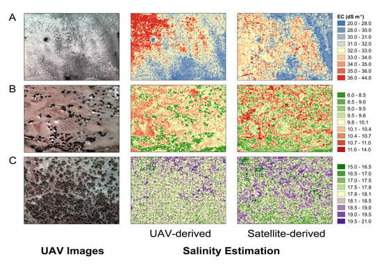
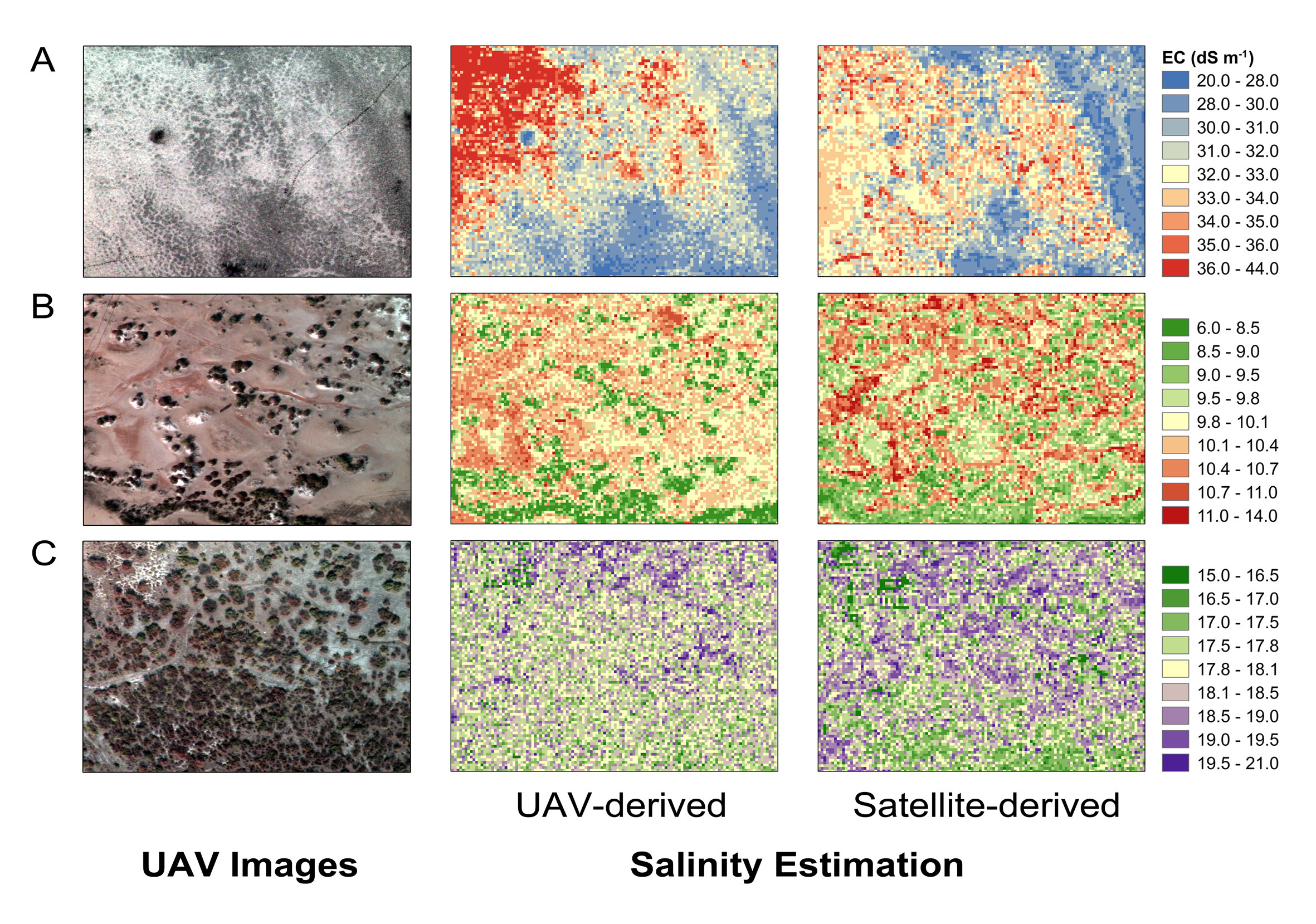
3.3. Soil Salinity Maps Derived from UAV and GF-2 Data

Figure 3 showed the soil salinity maps of the study areas developed using RF regression models. Since the resampled UAV data didn’t produce better prediction accuracy than the original UAV data did (Table 4), only the salinity maps derived from the original UAV and GF-2 data were shown to make comparisons. For both the UAV and GF-2 prediction models, the predicted EC values of fields A, B and C covered the range of around 20.0~44.0 dS m1, 6.0~14.0 dS m1, and 13.0~22.0 dS m1, respectively. In general, the maps of the field A (Figure 3a,b) and B (Figure 3c,d) showed distinct spatial variation pattern of soil salinity, whereas the GF-2 map of field C (Figure 3f) was too fragmented and scattered to recognize any salinity spatial pattern due to its dense vegetation cover.
The field A had the most extreme soil salinity. High salts (>35.0 dS m1) were mostly located in the northwest area (Figure 3a). An obvious difference was visible between the UAV and GF-2 models of the field A. For example, a large area with high salt content (>35.0 dS m−1) using the UAV model (Figure 3a) exhibited with relatively lower salt contents (32~35 dS m−1) using the GF-2 model (Figure 3b). In the UAV prediction map of the field B (Figure 3c), relatively high EC values (>10.4 dS m−1) were mostly found in the north and the west part of the study area, and EC values less than 9.0 dS m−1 were mainly distributed in the southern region and places with clustered populations of halophytes (Tamarix ramosissima). However, the GF-2 prediction map of the field B (Figure 3d) showed fewer areas of moderate EC values (9.8~10.4 dS m−1) and more areas of relatively high EC values (>11.0 dS m−1). In the soil salinity map of the field C derived from UAV data (Figure 3e), high salt content (>19.0 dS m−1) soils were located in the northeast part of the area. Compared with the UAV prediction map (Figure 3e), there was a greater area with EC values higher than 18.5 dS m−1 in the GF-2 prediction map of the field C.

4. Discussion

4.1. Comparison of RF Regression Models Based on UAV and GF-2

Accurate atmospheric correction was critical to remote sensing-based soil properties estimation as mainly atmospheric scattering distorted the real surface reflectance especially for the blue bands. However, conventional atmospheric correction methods for satellite images were not directly applicable for UAV-borne hyperspectral images. Although the lack of atmospheric correction may lead to inaccurate retrieval of soil salinity because of atmospheric perturbations, the Rikola camera we used did not capture data in the shortwave wavelength region less than 0.50 μm. The reflectance of the UAV-borne hyperspectral data was more detailed and intense than the reflectance of the satellite-borne multispectral data. Thus, the fully empirical approach with the RF can be applied without atmospheric correction. Even so, many researchers have tried to develop different radiometric correction methods especially for UAV-borne hyperspectral data. Honkavaara et al. [57] constructed a physically-based method which includes a radiometric block adjustment utilizing radiometric tie points and utilized in situ irradiance measurements. Lorenz et al. [58] performed a radiometric correction using a single atmospheric correction spectrum for each scene.
The RF regression modelling permitted reliable estimations and mapping of soil salinity at the field-scale (Table 4). The RF regression models using the UAV data source had higher CC and RPD values and lower RMSE values than the models using the GF-2 data source. This indicated that the 62-band hyperspectral images provided better prediction results than the multispectral GF-2 data in all three fields, despite lacking spectral information in the wavelength range from 0.45 to 0.50 μm. After spectral resampling, the accuracy of the UAV prediction models reduced, revealing that narrow bands, compared with broad bands, provide more detailed spectral information which could contribute to improving model performance. The RF regression models of field A were accurate with RPD values of 2.98 and 2.23, and the predictions of RF regression models of field B were good with RPD values of 2.15 and 2.00, but both the UAV and GF-2 prediction models of field C were ineffective as the RPD values were below 1.80 [59].
Because EMI measurements were conducted densely at field-scale, OOB and validation samples were often almost identical to samples used in the training of the models. It inevitably resulted in overestimation of the model’s prediction accuracy [60,61]. Even so, this study developed a novel approach of combining EMI and remote sensing techniques to map field-scale soil salinity. Our results presented relatively reliable spectral inversion of salinity in three fields with variable vegetation cover. In future research, spatial independence selection methods such as spatial blocking will be employed to conduct cross-validation in order to address the overoptimism of the prediction models.

4.2. Soil Salinity under Various Vegetation Cover Conditions

In this study, the highest surface soil EC value (47.14 dS m−1) was measured in the field A where no vegetation existed. However, although the field C had the densest vegetation cover, the soil salinity was generally higher than that of the field B where vegetation cover was sparse. It suggested that soil salinity was not simply negatively correlated with vegetation cover. As given in Table 2, the average soil salinity in the field C was above 15 dS m−1, which was much greater than the soil salinity in the field B. One possible reason is that halophytes, unlike other plants or crops, were adapted to moderate and even high contents of salt in soils. For the phreatophyte Tamarix ramosissima in the field B, their root could reach deep down in the soil, and the physiological activity and biomass accumulation majorly rely on the stable groundwater [62]. Moreover, for halophytes in the field C, their physiological characteristic enabled them to not only survive but also flourish with optimal growth in saline conditions that would kill other species [63].
With the increase of vegetation cover, the prediction performance of spectral retrieval models presented a decreasing trend with higher RMSE and lower CC and RPD values. It was reasonable because reflectance of the canopy rather than surface soil was collected via UAV. Although the canopy spectra did not directly depict the salt content in soils, it could be an indirect indicator of salinity. Under salt stress, the spectral reflectance and morphology of plant or crops on the ground would change due to insufficient water uptake and specific ion toxicity. Existing literatures have proposed methods to assess soil salinity using environmental indicators, including spectral vegetation indices such as normalized difference vegetation index (NDVI). Peng et al. [42] used a variety of environmental and ecological covariates, including NDVI, to quantitatively characterize the salinity of arid-area soils, the prediction accuracy of the cubist model was good with the R2, RMSE, MAE and RPD values of 0.91, 5.18 dS m−1, 3.76 dS m−1, and 3.15, respectively. In the Yellow River Delta of China, Zhang et al. [64] assessed the applicability of monitoring soil salinization utilizing vegetation indices derived from the MODIS time series data. Additionally, Allbed et al. [65] analyzed NDVI values and salinity index properties to monitor changes in soil salinity and vegetation cover from multispectral images. Further study about delineating soil salinity using salinity indices will be carried out to overcome the low prediction accuracy of models derived from a dense vegetation area.

4.3. Evaluation of the Variable Importance for Hyperspectral Soil Salinity Modeling

To understand which variables were the most significant among the 62 hyperspectral bands, variable importance analysis of RF regression models was utilized and the result was shown in Figure 4.
As shown in Figure 4, B18 (0.61 µm), B23 (0.65 µm), and B60 (0.87µm) were the most important bands for the UAV-derived prediction models of fields A, B, and C, respectively. They provided approximately 42%, 36%, and 34% increase in MSE for the regression models of the study area. It indicated that the red bands of fields A and B were of great significance, and the bands in the NIR spectral range were more important for field C when estimating soil salinity using UAV-derived hyperspectral data. As shown in Figure 4a, six of the top ten important bands for the prediction model of field A were NIR bands. The accumulated variable importance of NIR bands in Figure 4a reached up to 156%, suggesting that those bands are also critical to the modeling of soil salinity in the field A. The results were in accordance with the results of existing research. Sidike et al. [66] selected soil salinity sensitive bands using PLSR method, and the results indicated that the near-infrared band had the most contribution to the estimation of soil salinity. The statistical analysis of Fan et al. [67] demonstrated that soil salinity was more correlated with NIR and SWIR bands with larger negative correlation coefficients. Resulting from raw reflectance correlogram, first derivative reflectance correlogram, and PLSR carried out by Zhang et al. [68], wavelengths at 395~410, 483~507, 632~697, 731~762, 812~868, 884~909, and 918~930 nm were found to be the most sensitive wavebands. In the spectral range of 500~890 nm, wavelengths at 632~697, 731~762, and 812~868 nm covered B22~B31, B40~B47, and B53~B60 of the hyperspectral data in this research, respectively. Regarding to Figure 4, it was worth noticing that B23, B24, and B46 were among the top five most important hyperspectral bands for RF models in all three fields. Meanwhile, some NIR bands, including B53, B55, B56, B57, and B59, were all presented as important variables for RF model of the field A, as shown in Figure 4a.

5. Conclusions

This paper examined unmanned aerial vehicle-borne hyperspectral data and Chinese GF-2 satellite data for RF modeling to quantitatively estimate soil salinity in fields with various vegetation cover conditions. The strongest linear relationships between EM38-MK2-measured ECah, ECav, and laboratory-analyzed EC1:5 of the samples was found in the field C with R2 values 0.95. The bare land (field A) had the most saline soil, and its average EC1:5 of the soil samples was 37.64 dS m−1. The results showed that bare land with high salt content in soil had the most accurate estimation result among three fields. In addition, resampling UAV data to 1 m was necessary to get a reasonable relation to EMI measurements. For UAV-derived prediction models, the most important spectral band for salinity prediction was B18, B23, and B60 for the fields A, B, and C, respectively. Whereas B23, B24, and B46 were all significant to RF models of three fields. While the UAV platform was satisfactory for collecting spectral information to establishing regression models between EC and soil surface reflectance, soil salinity estimation achieved more accurate results for bare land and sparse vegetation area than dense vegetation area. As the acquired ultra-high-resolution images can capture details of ground objects, the UAV-borne hyperspectral imager was recommended for very accurate soil salinity mapping, monitoring and assessment in order to assist decision making in precision agriculture.

Author Contributions

Conceptualization, J.H., J.P. and Z.S.; Data curation, J.H. and R.Z.; Funding acquisition, J.P. and Z.S.; Investigation, J.P. and R.Z.; Methodology, J.H., J.P., Y.Z., and D.X.; Project administration, Z.S.; Resources, Q.J.; Software, D.X.; Supervision, Y.Z. and Z.S.; Visualization, J.H., Y.Z. and T.F.; Writing—original draft, J.H. and T.F.; Writing—review and editing, J.H., J.P., Y.Z., D.X., R.Z., Q.J., and F.W.

Funding

This research was funded by the National Key Research and Development Program of China (2016FYC0501400) and the National Natural Science Foundation of China (No. 41361048; No. 41261083).

Conflicts of Interest

The authors declare no conflict of interest. The funders had no role in the design of the study; in the collection, analyses, or interpretation of data; in the writing of the manuscript, or in the decision to publish the results.

References

  1. Dehni, A.; Lounis, M. Remote sensing techniques for salt affected soil mapping: Application to the oran region of algeria. Procedia Eng. 2012, 33, 188–198. [Google Scholar] [CrossRef]
  2. Ghassemi, F.; Jakeman, A.J.; Nix, H.A. Salinisation of Land and Water Resources: Human Causes, Extent, Management and Case Studies; CAB International: Wallingford, UK, 1995. [Google Scholar]
  3. Corwin, D. Past, Present, and Future Trends of Soil Electrical Conductivity Measurement Using Geophysical Methods; FAO: Rome, Italy, 2008. [Google Scholar]
  4. Ding, J.; Yu, D. Monitoring and evaluating spatial variability of soil salinity in dry and wet seasons in the werigan–kuqa oasis, china, using remote sensing and electromagnetic induction instruments. Geoderma 2014, 235–236, 316–322. [Google Scholar] [CrossRef]
  5. Guo, Y.; Huang, J.; Shi, Z.; Li, H. Mapping spatial variability of soil salinity in a coastal paddy field based on electromagnetic sensors. PLoS ONE 2015, 10, e0127996. [Google Scholar] [CrossRef] [PubMed]
  6. de Jong, E.; Ballantyne, A.K.; Cameron, D.R.; Read, D.W.L. Measurement of apparent electrical conductivity of soils by an electromagnetic induction probe to aid salinity surveys. Soil Sci. Soc. Am. J. 1979, 43, 810–812. [Google Scholar] [CrossRef]
  7. McNeill, J.D. Rapid, accurate mapping of soil salinity by electromagnetic ground conductivity meters. In Advances in Measurement of Soil Physical Properties: Bringing Theory into Practice; Topp, G.C., Reynolds, W.D., Green, R.E., Eds.; Soil Science Society of America: Madison, WI, USA, 1992; pp. 209–229. [Google Scholar]
  8. Corwin, D.L.; Lesch, S.M. Apparent soil electrical conductivity measurements in agriculture. Comput. Electron. Agric. 2005, 46, 11–43. [Google Scholar] [CrossRef]
  9. Guo, Y.; Shi, Z.; Li, H.Y.; Triantafilis, J. Application of digital soil mapping methods for identifying salinity management classes based on a study on coastal central china. Soil Use Manag. 2013, 29, 445–456. [Google Scholar] [CrossRef]
  10. Triantafilis, J.; Odeh, I.O.A.; McBratney, A.B. Five geostatistical models to predict soil salinity from electromagnetic induction data across irrigated cotton. Soil Sci. Soc. Am. J. 2001, 65, 869–878. [Google Scholar] [CrossRef]
  11. Csillag, F.; Pasztor, L.; Biehl, L.L. Spectral band selection for the characterization of salinity status of soils. Remote Sens. Environ. 1993, 43, 231–242. [Google Scholar] [CrossRef]
  12. Eldeiry, A.A.; Garcia, L.A. Detecting soil salinity in alfalfa fields using spatial modeling and remote sensing. Soil Sci. Soc. Am. J. 2008, 72, 201–211. [Google Scholar] [CrossRef]
  13. Kalra, N.K.; Joshi, D.C. Potentiality of landsat, spot and irs satellite imagery, for recognition of salt affected soils in indian arid zone. Int. J. Remote Sens. 1996, 17, 3001–3014. [Google Scholar] [CrossRef]
  14. Ben-Dor, E.; Metternicht, G.; Goldshleger, N.; Mor, E.; Mirlas, V.; Basson, U. Review of Remote Sensing-Based Methods to Assess Soil Salinity; Taylor & Francis Group: Abingdon, UK, 2009; pp. 39–60. [Google Scholar]
  15. Metternicht, G.I.; Zinck, J.A. Remote sensing of soil salinity: Potentials and constraints. Remote Sens. Environ. 2003, 85, 1–20. [Google Scholar] [CrossRef]
  16. Dwivedi, R.S.; Sreenivas, K. Image transforms as a tool for the study of soil salinity and alkalinity dynamics. Int. J. Remote Sens. 1998, 19, 605–619. [Google Scholar] [CrossRef]
  17. Hick, P.T.; Russell, W.G.R. Some spectral considerations for remote-sensing of soil-salinity. Aust. J. Soil Res. 1990, 28, 417–431. [Google Scholar] [CrossRef]
  18. Mougenot, B.; Pouget, M.; Epema, G.F. Remote sensing of salt affected soils. Remote Sens. Rev. 1993, 7, 241–259. [Google Scholar] [CrossRef]
  19. Verma, K.S.; Saxena, R.K.; Barthwal, A.K.; Deshmukh, S.N. Remote-sensing technique for mapping salt-affected soils. Int. J. Remote Sens. 1994, 15, 1901–1914. [Google Scholar] [CrossRef]
  20. Dehaan, R.L.; Taylor, G.R. Field-derived spectra of salinized soils and vegetation as indicators of irrigation-induced soil salinization. Remote Sens. Environ. 2002, 80, 406–417. [Google Scholar] [CrossRef]
  21. Douaoui, A.E.K.; Nicolas, H.; Walter, C. Detecting salinity hazards within a semiarid context by means of combining soil and remote-sensing data. Geoderma 2006, 134, 217–230. [Google Scholar] [CrossRef]
  22. Eldeiry, A.A.; Garcia, L.A. Comparison of ordinary kriging, regression kriging, and cokriging techniques to estimate soil salinity using landsat images. J. Irrig. Drain. Eng. Asce 2010, 136, 355–364. [Google Scholar] [CrossRef]
  23. Fernandez-Buces, N.; Siebe, C.; Cram, S.; Palacio, J.L. Mapping soil salinity using a combined spectral response index for bare soil and vegetation: A case study in the former lake texcoco, mexico. J. Arid Environ. 2006, 65, 644–667. [Google Scholar] [CrossRef]
  24. Ben-Dor, E.; Patkin, K.; Banin, A.; Karnieli, A. Mapping of several soil properties using dais-7915 hyperspectral scanner data—A case study over clayey soils in israel. Int. J. Remote Sens. 2002, 23, 1043–1062. [Google Scholar] [CrossRef]
  25. Cloutis, E.A. Hyperspectral geological remote sensing: Evaluation of analytical techniques. Int. J. Remote Sens. 1996, 17, 2215–2242. [Google Scholar] [CrossRef]
  26. Ghosh, G.; Kumar, S.; Saha, S.K. Hyperspectral satellite data in mapping salt-affected soils using linear spectral unmixing analysis. J. Indian Soc. Remote Sens. 2012, 40, 129–136. [Google Scholar] [CrossRef]
  27. Weng, Y.; Qi, H.; Fang, H.; Zhao, F.; Lu, Y. Plsr-based hyperspectral remote sensing retrieval of soil salinity of chaka-gonghe basin in qinghai province. Acta Pedol. Sin. 2010, 47, 1255–1263. [Google Scholar]
  28. Farifteh, J.; Van der Meer, F.D.; Atzberger, C.; Carranza, E.J.M. Quantitative analysis of salt-affected soil reflectance spectra: A comparison of two adaptive methods (plsr and ann). Remote Sens. Environ. 2007, 110, 59–78. [Google Scholar] [CrossRef]
  29. Pang, G.; Wang, T.; Liao, J.; Li, S. Quantitative model based on field-derived spectral characteristics to estimate soil salinity in minqin county, china. Soil Sci. Soc. Am. J. 2014, 78, 546–555. [Google Scholar] [CrossRef]
  30. Berni, J.A.J.; Fereres Castiel, E.; Suárez Barranco, M.D.; Zarco-Tejada, P.J. Thermal and narrow-band multispectral remote sensing for vegetation monitoring from an unmanned aerial vehicle. Ieee Trans. Geosci. Remote Sens. 2009, 47, 722–738. [Google Scholar] [CrossRef]
  31. Feng, Q.; Liu, J.; Gong, J. Uav remote sensing for urban vegetation mapping using random forest and texture analysis. Remote Sens. 2015, 7, 1074–1094. [Google Scholar] [CrossRef]
  32. Aasen, H.; Burkart, A.; Bolten, A.; Bareth, G. Generating 3d hyperspectral information with lightweight uav snapshot cameras for vegetation monitoring: From camera calibration to quality assurance. Isprs J. Photogramm. Remote Sens. 2015, 108, 245–259. [Google Scholar] [CrossRef]
  33. de Castro, A.I.; Torres-Sanchez, J.; Pena, J.M.; Jimenez-Brenes, F.M.; Csillik, O.; Lopez-Granados, F. An automatic random forest-obia algorithm for early weed mapping between and within crop rows using uav imagery. Remote Sens. 2018, 10, 285. [Google Scholar] [CrossRef]
  34. Lelong, C.; Burger, P.; Jubelin, G.; Roux, B.; Labbé, S.; Baret, F. Assessment of unmanned aerial vehicles imagery for quantitative monitoring of wheat crop in small plots. Sensors 2008, 8, 3557. [Google Scholar] [CrossRef] [PubMed]
  35. Ivushkin, K.; Bartholomeus, H.; Bregt, A.K.; Pulatov, A.; Franceschini, M.H.D.; Kramer, H.; van Loo, E.N.; Jaramillo Roman, V.; Finkers, R. Uav based soil salinity assessment of cropland. Geoderma 2019, 338, 502–512. [Google Scholar] [CrossRef]
  36. Romero-Trigueros, C.; Nortes, P.A.; Alarcón, J.J.; Hunink, J.E.; Parra, M.; Contreras, S.; Droogers, P.; Nicolás, E. Effects of saline reclaimed waters and deficit irrigation on citrus physiology assessed by uav remote sensing. Agric. Water Manag. 2017, 183, 60–69. [Google Scholar] [CrossRef]
  37. Zhao, K.; Song, J.; Feng, G.; Zhao, M.; Liu, J. Species, types, distribution, and economic potential of halophytes in china. Plant Soil 2011, 342, 495–526. [Google Scholar] [CrossRef]
  38. Heil, K.; Schmidhalter, U. Comparison of the em38 and em38-mk2 electromagnetic induction-based sensors for spatial soil analysis at field scale. Comput. Electron. Agric. 2015, 110, 267–280. [Google Scholar] [CrossRef]
  39. Peng, J.; Ji, W.; Ma, Z.; Li, S.; Chen, S.; Zhou, L.; Shi, Z. Predicting total dissolved salts and soluble ion concentrations in agricultural soils using portable visible near-infrared and mid-infrared spectrometers. Biosyst. Eng. 2016, 152, 94–103. [Google Scholar] [CrossRef]
  40. Roosjen, P.; Suomalainen, J.; Bartholomeus, H.; Kooistra, L.; Clevers, J. Mapping reflectance anisotropy of a potato canopy using aerial images acquired with an unmanned aerial vehicle. Remote Sens. 2017, 9, 417. [Google Scholar] [CrossRef]
  41. Adler-Golden, S.M.; Matthew, M.W.; Bernstein, L.S.; Levine, R.Y.; Berk, A.; Richtsmeier, S.C.; Acharya, P.K.; Anderson, G.P.; Felde, J.W.; Gardner, J.A.; et al. Atmospheric correction for shortwave spectral imagery based on modtran4. SPIE 1999, 3753, 61–69. [Google Scholar]
  42. Peng, J.; Biswas, A.; Jiang, Q.S.; Zhao, R.Y.; Hu, J.; Hu, B.F.; Shi, Z. Estimating soil salinity from remote sensing and terrain data in southern xinjiang province, china. Geoderma 2019, 337, 1309–1319. [Google Scholar] [CrossRef]
  43. Ho, T.K. The random subspace method for constructing decision forests. Ieee Trans. Pattern Anal. Mach. Intell. 1998, 20, 832–844. [Google Scholar]
  44. Breiman, L. Random forests. Mach. Learn. 2001, 45, 5–32. [Google Scholar] [CrossRef]
  45. Cutler, A.; Cutler, D.R.; Stevens, J.R. Random forests. In Ensemble Machine Learning: Methods and Applications; Zhang, C., Ma, Y., Eds.; Springer US: Boston, MA, USA, 2012; pp. 157–175. [Google Scholar]
  46. Cutler, D.R.; Edwards, T.C.; Beard, K.H.; Cutler, A.; Hess, K.T.; Gibson, J.; Lawler, J.J. Random forests for classification in ecology. Ecology 2007, 88, 2783–2792. [Google Scholar] [CrossRef] [PubMed]
  47. Mutanga, O.; Adam, E.; Cho, M.A. High density biomass estimation for wetland vegetation using worldview-2 imagery and random forest regression algorithm. Int. J. Appl. Earth Obs. Geoinf. 2012, 18, 399–406. [Google Scholar] [CrossRef]
  48. Were, K.; Bui, D.T.; Dick, Ø.B.; Singh, B.R. A comparative assessment of support vector regression, artificial neural networks, and random forests for predicting and mapping soil organic carbon stocks across an afromontane landscape. Ecol. Indic. 2015, 52, 394–403. [Google Scholar] [CrossRef]
  49. Liaw, A.; Wiener, M. Classification and regression by randomforest. R News 2002, 2, 18–22. [Google Scholar]
  50. R Core Team. R: A Language and Environment for Statistical Computing; R Foundation for Statistical Computing: Vienna, Austria, 2018. [Google Scholar]
  51. Forkuor, G.; Hounkpatin, O.K.L.; Welp, G.; Thiel, M. High resolution mapping of soil properties using remote sensing variables in south-western burkina faso: A comparison of machine learning and multiple linear regression models. PLoS ONE 2017, 12, e0170478. [Google Scholar] [CrossRef]
  52. Zhu, R.; Zeng, D.; Kosorok, M.R. Reinforcement learning trees. J. Am. Stat. Assoc. 2015, 110, 1770–1784. [Google Scholar] [CrossRef]
  53. Lawrence, I.K.L. A concordance correlation coefficient to evaluate reproducibility. Biometrics 1989, 45, 255–268. [Google Scholar]
  54. Zhou, Y.; Hartemink, A.E.; Shi, Z.; Liang, Z.; Lu, Y. Land use and climate change effects on soil organic carbon in north and northeast china. Sci. Total Environ. 2019, 647, 1230–1238. [Google Scholar] [CrossRef] [PubMed]
  55. Farifteh, J.; van der Meer, F.; van der Meijde, M.; Atzberger, C. Spectral characteristics of salt-affected soils: A laboratory experiment. Geoderma 2008, 145, 196–206. [Google Scholar] [CrossRef]
  56. Mashimbye, Z.E.; Cho, M.A.; Nell, J.P.; De Clercq, W.P.; Van Niekerk, A.; Turner, D.P. Model-based integrated methods for quantitative estimation of soil salinity from hyperspectral remote sensing data: A case study of selected south african soils. Pedosphere 2012, 22, 640–649. [Google Scholar] [CrossRef]
  57. Ji, W.J.; Li, S.; Chen, S.C.; Shi, Z.; Rossel, R.A.V.; Mouazen, A.M. Prediction of soil attributes using the chinese soil spectral library and standardized spectra recorded at field conditions. Soil Tillage Res. 2016, 155, 492–500. [Google Scholar] [CrossRef]
  58. Roberts, D.R.; Bahn, V.; Ciuti, S.; Boyce, M.S.; Elith, J.; Guillera-Arroita, G.; Hauenstein, S.; Lahoz-Monfort, J.J.; Schröder, B.; Thuiller, W.; et al. Cross-validation strategies for data with temporal, spatial, hierarchical, or phylogenetic structure. Ecography 2017, 40, 913–929. [Google Scholar] [CrossRef] [Green Version]
  59. Honkavaara, E.; Saari, H.; Kaivosoja, J.; Pölönen, I.; Hakala, T.; Litkey, P.; Mäkynen, J.; Pesonen, L. Processing and assessment of spectrometric, stereoscopic imagery collected using a lightweight uav spectral camera for precision agriculture. Remote Sens. 2013, 5, 5006–5039. [Google Scholar] [CrossRef]
  60. Lorenz, S.; Salehi, S.; Kirsch, M.; Zimmermann, R.; Unger, G.; Vest Sørensen, E.; Gloaguen, R. Radiometric correction and 3d integration of long-range ground-based hyperspectral imagery for mineral exploration of vertical outcrops. Remote Sens. 2018, 10, 176. [Google Scholar] [CrossRef]
  61. Le Rest, K.; Pinaud, D.; Monestiez, P.; Chadoeuf, J.; Bretagnolle, V. Spatial leave-one-out cross-validation for variable selection in the presence of spatial autocorrelation. Glob. Ecol. Biogeogr. 2014, 23, 811–820. [Google Scholar] [CrossRef] [Green Version]
  62. Xu, H.A.O.; Li, Y.A.N.; Xu, G.; Zou, T. Ecophysiological response and morphological adjustment of two central asian desert shrubs towards variation in summer precipitation. Plantcell Environ. 2007, 30, 399–409. [Google Scholar] [CrossRef] [PubMed]
  63. Flowers, T.J.; Colmer, T.D. Salinity tolerance in halophytes*. New Phytol. 2008, 179, 945–963. [Google Scholar] [CrossRef] [Green Version]
  64. Zhang, T.T.; Qi, J.G.; Gao, Y.; Ouyang, Z.T.; Zeng, S.L.; Zhao, B. Detecting soil salinity with modis time series vi data. Ecol. Indic. 2015, 52, 480–489. [Google Scholar] [CrossRef]
  65. Allbed, A.; Kumar, L.; Aldakheel, Y.Y. Assessing soil salinity using soil salinity and vegetation indices derived from ikonos high-spatial resolution imageries: Applications in a date palm dominated region. Geoderma 2014, 230, 1–8. [Google Scholar] [CrossRef]
  66. Sidike, A.; Zhao, S.; Wen, Y. Estimating soil salinity in pingluo county of china using quickbird data and soil reflectance spectra. Int. J. Appl. Earth Obs. Geoinf. 2014, 26, 156–175. [Google Scholar] [CrossRef]
  67. Fan, X.; Liu, Y.; Tao, J.; Weng, Y. Soil salinity retrieval from advanced multi-spectral sensor with partial least square regression. Remote Sens. 2015, 7, 488–511. [Google Scholar] [CrossRef]
  68. Zhang, T.T.; Zeng, S.L.; Gao, Y.; Ouyang, Z.T.; Li, B.; Fang, C.M.; Zhao, B. Using hyperspectral vegetation indices as a proxy to monitor soil salinity. Ecol. Indic. 2011, 11, 1552–1562. [Google Scholar] [CrossRef]
Figure 1. Location of study area and electromagnetic induction (EMI) measurements in fields A (a), B (b), and C (c) within the Xinjiang Autonomous Region.
Remotesensing 11 00736 g001
Figure 2. Scatter plots of measured versus predicted electrical conductivity (EC)-derived from RF regression models using UAV data for the field A (a,d), B (b,e), and C (c,f); the upper three (ac) are the training results; the lower three (df) are the validation results; the blue lines are the fitted lines and the red lines are the 1:1 lines.
Remotesensing 11 00736 g002
Figure 3. EC maps derived from RF regression models using UAV (the left three: a,c,e) and GF-2 (the right three: b,d,f) data for the field A (a,b), B (c,d), and C (e,f).
Remotesensing 11 00736 g003
Figure 4. Variable importance measured by percentage increase in mean squared error (MSE) for the UAV-derived prediction models of field A (a), B (b), and C (c).
Remotesensing 11 00736 g004
Table 1. Remote sensing sensors used for detection and mapping of soil salinity. UAV: unmanned aerial vehicle; NIR: near infrared.
SensorNo. of BandsSpectral Range (μm)Spatial ResolutionPlatform
Hyperspectral Imager62Visible and NIR0.1 mUAV
B1~62: 0.50–0.89(flight height: 154 m)
GF-25Visible and NIR1 m (Panchromatic)/
4 m (Multispectral)
Satellite
Band1: 0.45–0.52 (Blue)
Band2: 0.52–0.59 (Green)
Band3: 0.63–0.69 (Red)
Band4: 0.77–0.89 (NIR)
Panchromatic: 0.45–0.90
Table 2. Descriptive summary of electrical conductivity ECa and EC1:5 measured on the samples in fields A, B, and C.
FieldConductivityDescriptive Statistics (ECa, mS m−1;EC1:5, dS m−1)
NMinMaxMeanMedianStd.Dev.CV
AECah30571.15955.72765.05766.72119.0216%
ECav30598.151065.57846.74865.22144.5317%
EC1:53020.2554.9037.6435.809.2125%
BECah30450.201092.15830.47903.09200.5824%
ECav30585.671035.90824.51779.02154.2719%
EC1:5307.2014.6811.7311.912.3820%
CECah30695.861126.99890.15861.09136.5415%
ECav30560.17955.56778.00782.09118.9215%
EC1:5309.6419.6414.1114.502.9421%
Table 3. Descriptive summary of EC1:5 in fields A, B, and C.
FieldDescriptive Statistics (EC1:5, dS m−1)
NMinMaxMeanMedianStd.Dev.CV
A150018.8147.1431.5431.224.1713%
B15005.0415.209.8910.001.6417%
C150011.9825.9418.1318.372.1012%
Table 4. Training and validation statistics of random forest (RF) regression models. CC: concordance coefficient; RPD: ratio of performance to deviation; RMSE: root mean square error.
Data SetSourceABC
CCRPDRMSECCRPDRMSECCRPDRMSE
(dS m−1) (dS m−1) (dS m−1)
Training (n = 1000)UAV0.963.921.050.943.290.490.811.911.07
GF-20.932.931.400.922.750.580.741.671.22
Resampled UAV0.953.221.280.922.720.590.701.551.31
Validation (n = 500)UAV0.942.981.400.862.150.740.561.291.59
GF-20.882.231.870.842.000.800.441.201.71
Resampled UAV0.892.351.780.811.850.860.401.121.83

