Article

Improving Aboveground Biomass Estimation of Pinus densata Forests in Yunnan Using Landsat 8 Imagery by Incorporating Age Dummy Variable and Method Comparison

1
Key Laboratory of State Forestry Administration on Biodiversity Conservation in Southwest China, Southwest Forestry University, Kunming 650224, China
2
Department of Geography, Southern Illinois University, Carbondale, IL 62901, USA
*
Author to whom correspondence should be addressed.
Remote Sens. 2019, 11(7), 738; https://doi.org/10.3390/rs11070738
Submission received: 26 January 2019 / Revised: 21 March 2019 / Accepted: 22 March 2019 / Published: 27 March 2019

Abstract

:
Optical remote sensing data have been widely used for estimating forest aboveground biomass (AGB). However, the use of optical images is often restricted by the saturation of spectral reflectance for forests that have multilayered and complex canopy structures and high AGB values and by the effect of spectral reflectance from underlayer shrub, grass, and bare soil for young stands. This usually leads to overestimations and underestimations for smaller and larger values, respectively, and makes it very challenging to improve the estimation accuracy of forest AGB. In this study, a novel methodology was proposed by incorporating stand age as a dummy variable into four models to improve the estimation accuracy of the Pinus densata forest AGB in Yunnan of Southwestern China. A total of eight models, including two parametric models (LM: linear regression model and LMC: LM with combined variables), two nonparametric models (RF: random forest and ANN: artificial neural network) without the age dummy variable, and four corresponding models with the age dummy variable (DLM, DLMC, DRF, and DANN), were compared to estimate AGB. Landsat 8 Operational Land Imager (OLI) images and 147 sample plots were acquired and utilized. The results showed that (1) compared with the two parametric models, the two nonparametric algorithms resulted in significantly greater estimation accuracies of Pinus densata forest AGB, and the increases of accuracy varied from 8% to 32% for 100 modeling plots and from 12% to 35% for 47 test plots based on root mean square error (RMSE); (2) compared with the models without the age dummy variable, the models with the age dummy variable greatly reduced the overestimations for the plots with AGB values smaller than 70 Mg/ha and the underestimations for the plots with AGB values larger than 180 Mg/ha and, thus, significantly improved the overall estimation accuracy by 14% to 42% for the modeling plots and by 32% to 44% for the test plots based on RMSE; and (3) the texture measures derived from the Landsat 8 OLI images contributed more to improving the estimation accuracy than the original spectral bands and other transformations. This implied that two nonparametric models, coupled with the use of the age dummy variable and texture measures, offered a great potential for improving the estimation accuracy of Pinus densata forest AGB.

Graphical Abstract

1. Introduction

As forest ecosystems play an important role in global carbon cycling and the mitigation of carbon concentrations in the atmosphere, accurately estimating forest biomass is necessary and has been widely studied [1,2,3,4,5,6,7,8]. Due to the difficulty and high cost of collecting field data, especially belowground biomass, most of the existing studies have focused on forest aboveground biomass (AGB) [9,10,11,12,13,14,15,16,17] and the use of remotely sensed data [18,19,20]. However, the estimation accuracy of forest AGB varies depending on many factors, including the remotely sensed images, the independent variables used, and the algorithms used to model the relationship of AGB with the independent variables [9].
As remote sensing technologies develop, various image data from Landsat, SPOT, QuickBird, IKONOS, WorldView, ASTER, MODIS, AVHRR, Radarsat, and ALOS PALSAR have become available and are used for AGB estimation [9]. Many studies have also investigated the data fusion of different sensor images for improving AGB estimation [21,22]. Given a study area, what kind of sensor data should be selected has become very challenging during the past several decades [23]. Overall, Landsat imagery has been most widely used for this purpose because of free downloading, a long-time history, large coverage, and medium spatial and temporal resolutions [9,21,24,25,26,27]. Especially, the new Landsat 8 provides images with more spectral bands and a higher radiometric resolution than previous Landsat satellites and, thus, a greater potential for improving AGB estimation [12,28].
Selecting spectral variables that have strong relationships with forest AGB is the key to increasing the accuracy of AGB estimation using remote sensing data [9,12,19,26]. Various spectral bands and other potential variables derived from the bands, such as vegetation indices, various transformations, texture measures, and fractional images have been used to construct the estimation models of forest AGB [9,24,26]. Generally, the models with the combinations of vegetation indices, texture measures, and environmental variables such as elevation, slope, and aspect can lead to higher estimation accuracy than those with original bands, and this is especially true for the forests with complex canopy structures [9,12,19,21].
Various parametric and nonparametric algorithms have been developed for mapping forest AGB using remotely sensed images [9,19]. Simple linear regression models (LMs) and nonlinear models such as power models [29,30] and logistic regression models [31] are often used. The LMs account for the relationships between forest AGB and predictors and are the most popular statistical models [9,32]. However, the relationships are often nonlinear and show power, exponential, or logarithmic forms. The nonlinear regression models or the linearization of the nonlinear relationship are common methods to deal with the nonlinear relationships. However, the determination coefficients obtained are often smaller than 0.5 [27,33], and the estimates obtained are, thus, not reliable [32].
Nonparametric models are an alternative approach to improve the estimation accuracy of forest AGB using remote sensing images. Many nonparametric algorithms, such as artificial neural networks (ANN) [34,35], random forest (RF) [36,37], k-Nearest Neighbors (kNN) [38], support vector machine (SVM) [39,40], and Maximum Entropy (MaxEnt) [41,42], have been explored to model the relationships between forest AGB and predictors. However, the model structures derived from these algorithms are often difficult to interpret [9,19,32]. The RF, introduced by Leo Breiman [43], can be used for either classifying categorical variables or estimating continuous variables such as forest AGB [43,44]. It provides the average prediction from a number of regression models created by a subset of training data selected randomly with a random subset of predictors [45,46]. Recently RF has been frequently used in AGB estimation by integrating the samples from field inventories, remote sensing, and other predictors [47,48]. Moreover, ANN, proposed in 1943, is a mathematical model inspired by biological neural networks. Its algorithm is the product of artificial intelligence as black-box models due to unknown weights and a difficulty in terminating the learning process [49]. Therefore, it has a strong ability for fitting the data [50] and provides a robust solution for complex and nonlinear problems due to its universal approximation properties [24]. Many different neural network models have been developed [51] and are widely used in various fields [52]. Unfortunately, the estimation accuracy of the nonparametric models is very much limited by the used sample sizes.
Moreover, forest AGB estimates derived from remote sensing data are associated with uncertainties [19], which has been widely recognized and for which substantial research has been conducted [53,54]. The uncertainties often result in underestimations for forests with great AGB values and overestimations for forests with small AGB values. The underestimations usually occur when AGB reaches 100–150 Mg/ha [33,55,56], while the overestimations often happen for forests with AGB less than 40 Mg/ha [33]. Many studies have indicated that the uncertainties are related to the structures of forest ecosystems, the topographic characteristics, the remotely sensed data (insensitivity and saturation) and their spatial resolutions, and the methods used [33,56,57,58,59,60,61,62]. Especially, spectral reflectance due to data saturation becomes less sensitive to AGB changes in the dense, multilayer, and complex canopy forest ecosystems and often leads to the underestimations of forest AGB [19]. Few studies have analyzed the saturation values of forest AGB for different forest ecosystems, and only a few reports have demonstrated methods to reduce the impact of data saturation on AGB estimation accuracy [20,22,33].
The heterogeneity of complex forest canopy structures may be the major impact for the data saturation and underestimation for the forests with high AGB values [22]. The data saturation varies depending on vegetation types because of the characteristics of their surface reflectance, including tree species, ages, and forest canopy structures [19,63]. Zhao et al. [22] analyzed the saturation values using Landsat imagery for different vegetation types, slopes, and aspects in a subtropical region of China; estimated AGB considering the stratification of forest types using a stepwise linear regression; and improved the estimation accuracy of AGB. The stratification of forest types based on tree species and environmental variables can provide the potential of improving the estimation of forest AGB [22,32,33]. Moreover, incorporating the tree age into the estimation models can also lead to an improvement of the AGB/carbon sequestration estimates and can reduce the overestimation and underestimation [64,65,66,67,68].
Iizuka and Tateishi [64] and Sanga-Ngoie et al. [68] introduced tree volume-derived age into tree carbon estimation models for improving the estimation accuracy of tree carbon sequestration using optical remote sensing imagery. Moreover, Zheng et al. [65] used 60 sample trees to obtain a forest stand age map in which the ages for most of the forests were less than 21 years old, then developed a polynomial model with spectral variables from Landsat ETM+ images and stand age involved, and obtained a high estimation accuracy of AGB. Lefsky et al. [66] mapped the forest stand age using the time series of Landsat images, then estimated the AGB of young stands using Lidar data in western Oregon, USA, and found that the estimation models were appropriate for the forests with the classes of ages 14.5 to 20.5 years but resulted in overestimations for the smaller age classes. Based on the years in which the trees were planted, Liu et al. [67] also obtained and added the age variable into their linear regression models to estimate the AGB of plantations using Landsat images. The studies indicate that taking tree ages into account would obtain a considerable improvement in estimating AGB. The studies dealt with reducing the overestimation of AGB for young forests, but the reports related to the improvement of the underestimation for the forests with high AGB values are still lacking.
Overall, the overestimation and underestimation of forest AGB commonly exist when optical remote sensing imagery is used. Reducing the overestimation and underestimation is critical to increase the estimation accuracy of forest AGB but is greatly challenging. The objective of this study was to develop a novel method of reducing the overestimation and underestimation to improve the accuracy of estimating forest AGB when optical images were utilized. The improvement was explored first by using Landsat 8 OLI images and four models to estimate AGB, including two parametric models: LM and a LM with combined variables (LMC), and two nonparametric models: RF and ANN. The stand group age as a dummy variable was then introduced into the four models, which led to four new models with the age dummy variable involved. Moreover, the eight models were compared for the estimation performance of forest AGB, and the significant contributions of adding the age dummy variable into the models to mitigating the overestimation and underestimation were statistically examined. The analyses and examinations were conducted in Pinus densata forests distributed in Yunnan of Southwestern China.

2. Materials and Methods
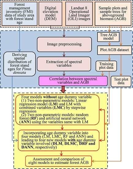
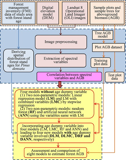
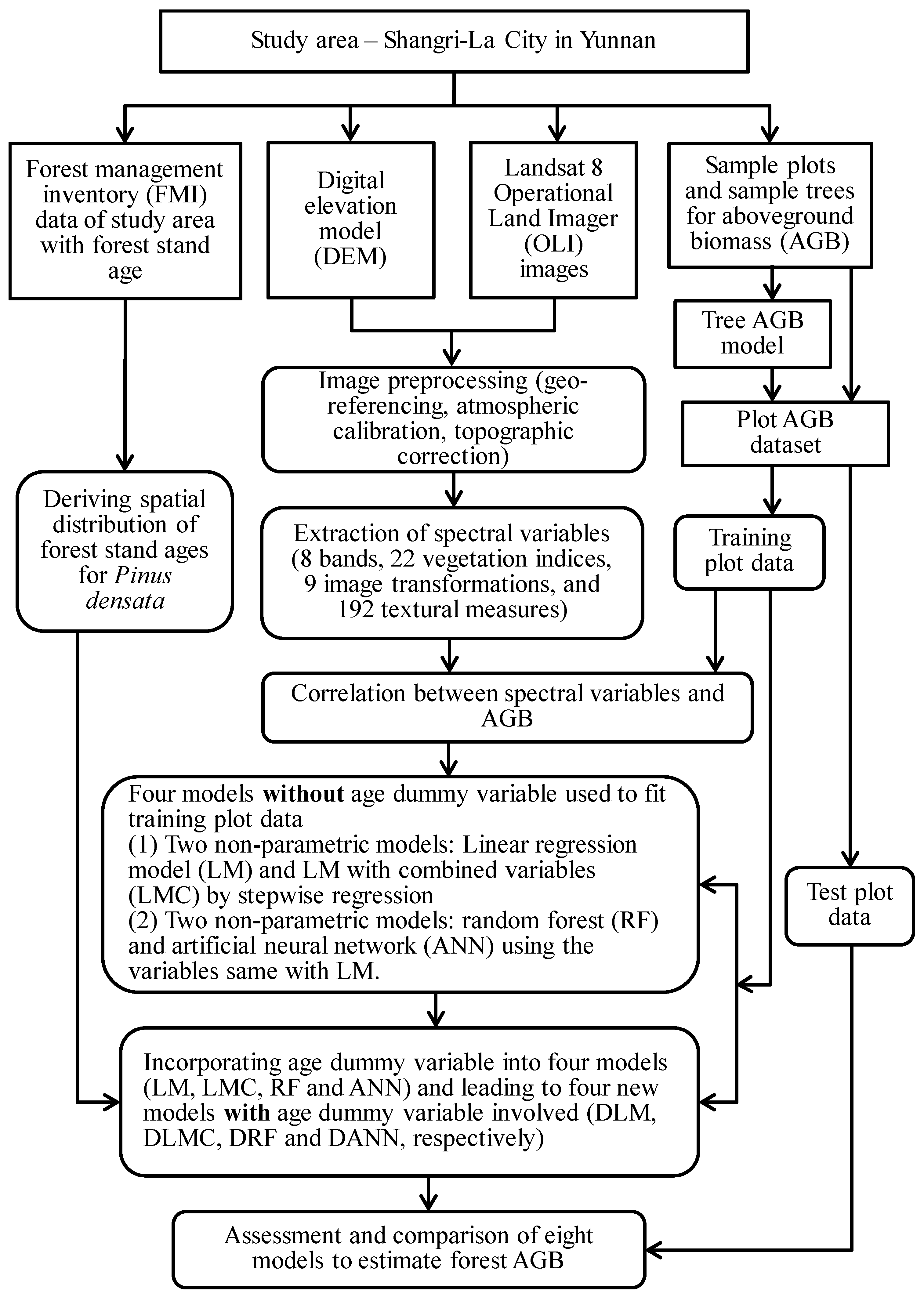
In Figure 1, the methodologic framework of this study is illustrated, consisting of the following steps: 1) the selection of the study area; 2) the collection of the sample plot and tree biomass data; 3) the calculation of the tree and plot AGB; 4) the acquisition, preprocessing, and analysis of the Landsat 8 OLI images; 5) the development of the models by incorporating the age dummy variable; and 6) the assessment and comparison of the forest AGB predictions from the models with and without the age dummy variable.

2.1. Study Area

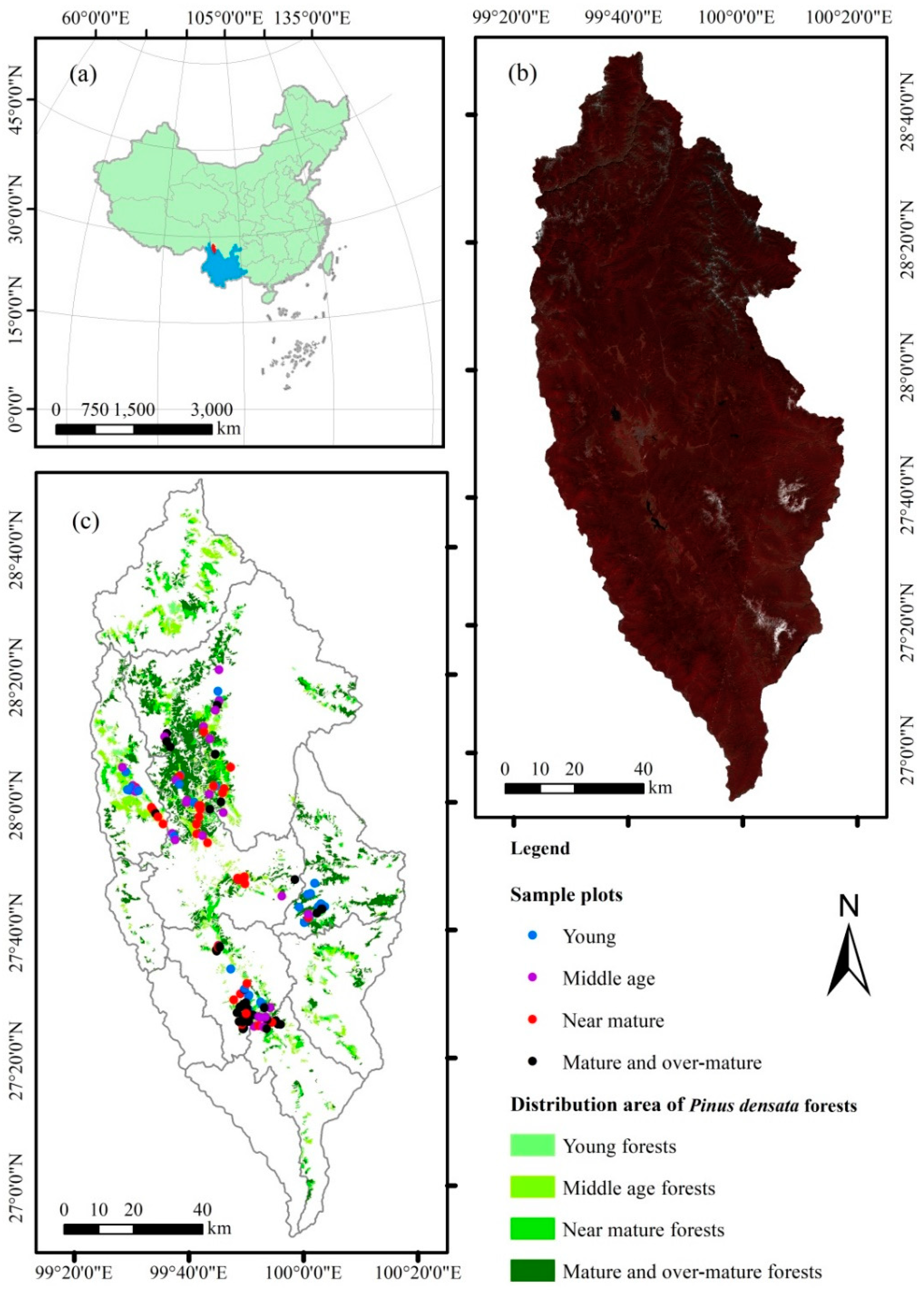
The study area is located in Shangri-La City, northwestern Yunnan of Southwestern China, and the AGB of Pinus densata forests were mapped (Figure 2). The study area is characterized by a cold temperate zone with the mean altitude of 3459 m above sea level. The annual mean temperature is about 5.4 °C with the monthly highest and lowest temperature of 13.3 °C in July and −3.8 °C in December, respectively. The winters are chilly but sunny because of the high altitude. The annual mean precipitation is about 607 mm. The seasonal distribution of precipitation is uneven with 70% in the rainy season (June–September). The evaporation is about 1671 mm per year, and the relative humidity is about 70%. The soil type is mainly dark brown forest soil [69]. The study area is dominated by cold, temperate coniferous forests with dominant tree species of Pinus, Picea, Larix, and Abies.
Pinus densata is an endemic and pioneer tree species for reforestation at the subalpine and alpine areas in the Hengduan Mountains [70]. It is a typical cool-temperature coniferous tree species distributed between cold-temperature coniferous forests dominated by Picea, Abies, and Larix and warm-temperature coniferous forests dominated by Pinus yunnanensis and P. armandii. In the study area, most of the forests are pure with a single canopy layer dominated by Pinus densata or mixed with small amount of Quercus pannosa, Pinus armandii, Picea likiangensis, Larix potaninii var. macrocarpa, and Betula spp., with the altitude ranging from 3000 m to 3700 m.

2.2. Measurement and Calculation of Aboveground Biomass for Sample Trees and Plots

A total of 147 square sample plots were measured in the field in 2017. The plots were selected in the P. desata pure forests of the study area by considering the stand ages, elevation, slope, and aspect, and the sampling distances between the plots were about 1 km (Figure 2). Each plot had an area of 30 m × 30 m, and its coordinates of location, elevation, slope, and aspect were measured. Within each plot, the diameter at breast height (1.3 m above ground) (DBH) and height (H) of each tree were recorded. The stand age (SA) of each plot is the mean age of three standard trees having similar DBH values to the average DBH of the plot. The ages of the three trees were measured by counting the annual rings on the wood cores obtained by a growth cone at the tree base.
Moreover, a spatial distribution map of the Pinus densata forest stand ages for the study area was obtained from the Shangri-La City forest inventory conducted in 2016 for forest management and planning. In the forest inventory, a spatial distribution map of forest types, that is, stand compartments, was produced in the field using visual interpretation based on aerial photographs. The compartments had similar dominant tree species and homogeneous canopy structures. Within each of the forest compartments, a certain number of 25.8 m × 25.8 m plots were selected, and within each of the plots, the DBH of each tree was measured and the average DBH was obtained. Then, 3 to 5 trees having a DBH similar to the plot average DBH were selected to measure the tree ages by counting the layers of branches along the tree trunk because the growth of Pinus densata trees is characterized by adding a layer of branches each year.
In addition, a total of 100 sampling trees were selected from the 147 sample plots to measure tree AGB. The selection of the sample trees was based on their DBH classes from 6 cm to 76 cm with a 2 cm interval and on their elevation, slope, and aspect. At least three sample trees were obtained for each of the DBH classes. The values of the tree AGB components including wood, bark, branches, and needles were obtained according to the method of Wang [71]. The biomass samples of wood and bark for each sample tree were collected by taking a 3 cm thickness disk at a 2 m interval along the tree trunk. The biomass values of each stem and its bark were measured by a method of volume and density. The volumes of the wood segments and barks were calculated using their lengths and diameters of the surfaces and under the barks. The samples of branches and leaves were selected, collected, and weighted by the method of graded branches. All the samples were dried to constant weights at 105 °C using an oven, and the sample density values of wood and bark were measured using a drainage method. Finally, the biomass values of wood and bark for the sample trees were calculated using the volumes and the corresponding sample density values. The branch and needle biomass of the sample trees were obtained using the ratios of fresh weight to the corresponding dry matter.
The AGB data of the individual sample trees (Unit: kg) were fit using a power function, and the AGB of each plot (Unit: Mg/ha) was summed using following Equation (1).
A G B s = i = 1 n A G B i 900 · 10000 / 1000
where AGBs is the AGB of a plot, AGBi is the estimated AGB of tree i, and n is the number of trees within the plot. Although the biomass samples of tree components were used, in fact, the biomass values of the sample trees and plots were associated with uncertainties and should be considered as reference values.

2.3. Remote Sensing Data and Preprocessing

Three Landsat 8 Operational Land Imager (OLI) images obtained from the website of the United States Geological Survey (USGS) were used in this research (Table 1). The images were geo-referenced to a Universal Transverse Mercator coordinate system with zone 47 north with a root mean square error (RMSE) of less than one pixel. An atmospheric calibration of the images was conducted using the dark object subtraction approach [72], and their topographic correction was made using the C-correction approach using a digital elevation model (DEM) at a spatial resolution of 30 m × 30 m [73,74]. The images were then mosaicked and clipped according to the study area (Figure 2b).
A total of 231 remote sensing variables were derived (Table 2), and they included 8 bands, 22 vegetation indices, 9 image transformations, and 192 textural measures (including mean, variance, homogeneity, contrast, dissimilarity, entropy, angular second moment, and correlation on seven bands with three moving window sizes: 3 × 3, 5 × 5, and 7 × 7 pixels). Vegetation indices and image transformations have been widely used in the estimation of forest AGB, and the texture measures were selected to capture the forest canopy structures [32]. The relationships between the spectral variables and AGB were analyzed using a Pearson correlation analysis, and the spectral variables with significant correlations (p ≤ 0.05) were selected to build the AGB estimation models.

2.4. Modeling Methods

Four models including LM, LMC, RF, and ANN were compared to estimate the AGB of the Pinus densata forests. The spectral variables that had statistically significant correlations with plot AGB were selected to develop the LM model by a stepwise regression with the variance inflation factor (VIF) of 10 to test the collinearity of the independent variables. In addition to the spectral variables above, logarithmic, quadratic, and cubic transformations were calculated for each spectral variable and used as the combined variables to construct the LMC model using a stepwise regression with VIF of 10. The introduction of the combined variables provided the potential to model the nonlinear relationship of AGB with the spectral variables. The modeling of RF was carried out by the Random Forest package in R software. Both the number of regression trees (ntree) and the number of input variables per node (mtry) were set, the optimal ntree was determined by bootstrap and RMSE, and the mtry was tested from one-third of all the independent variables [43]. Finally, we used the neuralnet package in R software to develop the ANN model. The number of nodes and layers for the models was set according to the default of the package, and the number of hidden layers was adjusted according to the predicted results. In addition, the independent variables used for ANN and RF were the same as those utilized for LM.

2.5. Modeling Methods with Age Dummy Variable

In this study, the sample plots were grouped into young stand, middle age stand, near-mature stand, mature stand, and overmature stand according to the stand ages (SA) of the Pinus densata forests. The age intervals of young stand, middle age stand, near-mature stand, mature stand, and overmature stand were SA ≤ 20 years, 20 years < SA ≤ 30 years, 30 years < SA ≤ 40 years, 40 years < SA≤ 60 years, and SA > 60 years, respectively. The age intervals of the stand groups were determined according to the growth rate and forest management objectives of Pinus densata. In this region, Pinus densata forests with the age range of 40 to 60 years are considered as wood mature with the maximum annual value and can be harvested [75,76]. Whether the stand age was used as a dummy variable and included into the models (LM, LMC, ANN, and RF) of AGB prediction and whether the potential combination of neighboring age groups was made were determined by following steps:
(1) The models LM, LMC, ANN, and RF were developed and used to predict the AGB values of both the modeling and test plots;
(2) The predictions of AGB were compared with the reference values from the field plots, and the mean residuals of the predictions were statistically tested for their significant differences from zero at the significance level of 0.05 based on each of the stand age groups;
(3) Given a stand group and a model, the existence of the significant difference implied an overestimation or underestimation, and the age of the stand group as a dummy variable was, thus, added into the model; otherwise, the age dummy variable was not involved;
(4) The models with the age dummy variable were developed, the significant difference tests of the obtained mean residuals from zero were conducted, and the reduction of the error was analyzed; and
(5) When the models without the age dummy variable led to the mean residuals that were not significantly different from zero at the significance level of 0.05 for two neighboring age groups, the sample plots of the neighboring age groups were combined and the above four steps were repeated using the combined dataset.
Based on the results, the forest stands were divided into four groups: young stand, middle-age stand, near-mature stand, and mature and overmature stand in which the stand group ages were used as a dummy variable and added into the models.

2.6. Assessment and Validation of Predictions from Models

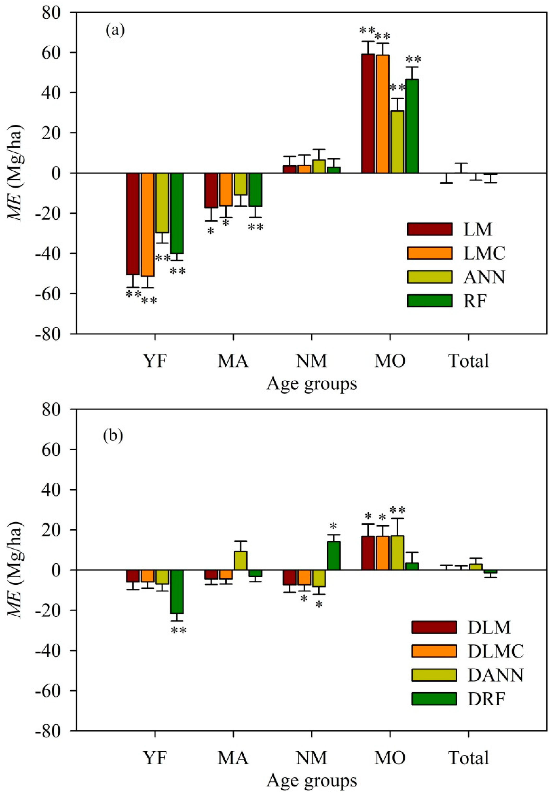
The evaluation of the obtained AGB models and the corresponding estimates was conducted using a determination coefficient (R2) and RMSE between the observed values and estimated values of AGB to assess and validate the models based on the plot dataset used for model fitting. Moreover, the applicability of the models was also validated using the test dataset with the mean error (ME) defined as the average value of the residuals (observed values minus estimated values). The mean error of each age group for the different estimation models was statistically tested for its significant difference from zero at the significance level of 0.05 using single sample t-test by SPSS. Among the 147 plots, 100 plots were randomly selected and used for the model fitting and 47 plots were used for the validation of the models.

3. Results

3.1. Statistical Characteristics of Sample Plot Data

The AGB values of individual sample trees were graphed against their DBH and H values, and the relationships of tree AGB with both DBH and H could be fit using a power function. Figure 3 shows the relationship for DBH, and the corresponding relationship for H was omitted. The obtained model with the determination coefficient of 0.992 and the RMSE of 30.778 kg was as follows:
AGB = 0.073·DBH1.739·H0.880
The AGB values of the trees within each plot (Unit: Mg/ha) were estimated using this equation, and the AGB value of each sample plot was obtained using Equation (1).
The statistics of plot AGB values were shown based on stand age groups in Table 3. The stand ages of the modeling plots, test plots, and all the sample plots were 37.77 years, 38.02 years, and 37.85 years with the maximum AGB values of 344.38 Mg/ha, 235.35 Mg/ha, and 344.38 Mg/ha, respectively. Their sample means were 112.15 Mg/ha, 115.43 Mg/ha, and 113.20 Mg/ha with the variation coefficients of 54.25%, 49.21%, and 52.47%, respectively. The sample means were not significantly different from each other at the significance level of 0.05.

3.2. Correlation between Spectral Variables and AGB

In this study, the Pearson correlation coefficients between all 231 spectral variables and the plot forest AGB were calculated. It was found that only 36 spectral variables had statistically significant correlations with plot forest AGB and are listed in Table 4, including 28 texture measures, 7 vegetation indices, and 1 component of PCA. The variance texture measure of band 4 using window size 3 × 3 pixels (VA3_4) and the angular second moment of band 1 with window size of 7 × 7 pixels (SM7_1) had the highest correlation. The absolute values of the correlation coefficients varied from 0.200 to 0.326. Overall, the texture measures had higher correlations with AGB than other spectral variables.

3.3. Model Fitting

3.3.1. Models without Age Dummy Variables

Four models, LM, LMC, RF, and ANN, were used to fit the modeling dataset, and their results are listed in Table 5. By a linear stepwise regression, the correlation texture measure for band 7 using the window size 7 × 7 (CC7_7), the variance texture measure for band 4 using the window size at 3 × 3 (VA3_4), the angular second moment texture measure for band 1 using the window size 5 × 5 (SM5_1), the dissimilarity texture measure for band 1 using the window size 5 × 5 (DI5_1), and structure insensitive pigment index (SIPI) were selected for LM. For LMC, the selected variables included quadratic VA3_4 ((VA3_4)2), cubic SM5_1 ((SM5_1)3), logarithmic entropy for band 1 using the window size at 5×5 (Log(EN5_1)), and SIPI. The spectral variables used for LM were also utilized for developing the models ANN and RF.
The results showed that both parametric models, LM and LMC, had smaller values of R2 and larger values of RMSE than the two nonparametric methods, RF and ANN. The ANN led to the largest R2 (0.663) and smallest RMSE (35.158 Mg/ha). The determination coefficient R2 from ANN was statistically significantly larger, and its RMSE was significantly smaller than those from LM and LMC. However, the R2 and RMSE values from ANN were not significantly different from those obtained by RF. The LMC only slightly improved the estimates compared with LM based on their RMSE values. This indicated that ANN provided the most accurate estimates of AGB, then RF, LMC, and LM.
Similar results were noticed in the scatter graphs of the predicted AGB values against the referenced values in Figure 4. The scatter graphs from ANN and RF had a narrower distribution and looked closer to the line of y = x than those scatter graphs from LMC and LM. For all the four models, however, there were overestimations when the plot AGB values were smaller than about 70 Mg/ha and underestimations when the plot AGB values were greater than about 180 Mg/ha. The only difference was that, compared with LMC and LM, the ANN and RF resulted in slightly smaller overestimations and underestimations.

3.3.2. Models with Age Dummy Variables

Overall, two nonparametric models, ANN with age dummy variable (DANN) and RF with age dummy variable (DRF), had a larger R2 and a smaller RMSE than the wo parametric models, LM with age dummy variable (DLM) and LMC with age dummy variable (DLMC) (Table 6). The DRF had the largest R2 and smallest RMSE, followed by DANN, then DLMC, and then DLM. Compared with the models without the age dummy variable, all the models with the age dummy variable greatly increased the coefficients of determination R2 and reduced the RMSE values. Compared with the corresponding models without the age dummy variable, the DLM led to the greatest increase of R2, then DLMC, DRF, and DANN. The DRF resulted in the greatest decrease of RMSE, then DLMC, DLM, and DANN. The improvements were also noticed by the scatter graphs of the predicted AGB values against the plot referenced values in Figure 5. The overestimations still happened for the plots with AGB values smaller than about 50 Mg/ha, and the underestimations occurred for the plots with AGB values larger than 190 Mg/ha for both DLMC and DLM (Figure 5a,b) and 200 Mg/ha for both DRF and DANN (Figure 5c,d). However, the overestimations and underestimations greatly decreased by the models with the age dummy variable compared with the models without the age dummy variable. In addition, compared with those without the age dummy variable, the models with the age dummy variable slightly reduced the predicted AGB values of the plots at which the overestimations existed and slightly increased the predicted AGB values of the plots at which the underestimations occurred.

3.4. Model Validation

In this study, we conducted the validation of the models with and without the age dummy variable based on the test dataset. For both the young and middle-age stands, the negative mean errors of the predictions from all the models without the age dummy variable except for ANN in the middle-age forests were statistically significantly different from zero (Figure 6a), indicating that the overestimations were statistically significant. Introducing the age dummy variable into the models significantly reduced the residuals and the resulting mean errors (that is, overestimations), except that from the model DRF became not significantly different from zero (Figure 6b). For the near-mature stand, the positive mean errors (underestimations) did not significantly differ from zero for all the models without the age dummy variable, and the models with the age dummy variable slightly deteriorated the estimations of the plot AGB. For the mature and overmature stand, the LM, LMC, ANN, and RF resulted in positive mean errors, that is, underestimations, being significantly different from zero at the significance level of 0.01. The models DLM, DLMC, DANN, and DRF greatly mitigated the underestimations but were still statistically significant at the significance level of 0.05 for DLM and DLMC and at the significance level of 0.01 for DANN. For all the test plots, the overall mean errors were not significantly different from zero at the significance levels of 0.05 for all the models with and without the age dummy variable.
Compared with the coefficients of determination R2 obtained using the models without the age dummy variables, the models with the age dummy variable increased the correlations between the referenced and predicted values of AGB for all the age group stands, but the increases were slight (Table 7). However, for the pooled test dataset, the increases were significant for all the models with the age dummy variable except for the DRF. Moreover, all the models with the age dummy variable significantly decreased the values of RMSE compared with those without the age dummy variable for all the age group stands and the pooled dataset. The decreases of RMSE using DLM, DLMC, DANN, and DRF were 69%, 71%, 69%, and 47% for the young stand; 45%, 47%, 53%, and 39 % for the mature and overmature stands; and 41%, 44%, 38%, and 32% for the pooled dataset, respectively. The decreases of RMSE for the middle-age stand and near-mature stand were relatively smaller and varied from 12% to 21%. There were also three exceptions: DANN increased the values of RMSE by 4% and 7% for the middle-age stand and near-mature stand and DRF increased the RMSE value by 6% for the near mature stand compared with the corresponding models, ANN and RF. Overall, the amount of RMSE decreases and the portion of R2 accounted for by adding the age dummy variable within the models decreased with the increase of the model performance without the age dummy variable.
Finally, the maps of the predicted AGB values for the Pinus densata forests were generated using all eight models in Figure 7. For the models with the age dummy variable, in addition to the selected spectral variables, the spatial distribution map of the Pinus densata forest stand ages obtained from the Shangri-La City forest inventory was used. Overall, the spatial distributions of the predicted AGB values by the models with the age dummy variable, especially by DANN and DRF, were more heterogeneous than those by the models without the age dummy variables, implying that the models with the age dummy variable reduced the overestimations for the smaller AGB values and the underestimations for the larger AGB values and, thus, increased the heterogeneity of the predicted AGB values.

4. Discussion

4.1. Remote Sensing Variables

Optical remote sensing data are commonly used for biomass estimation due to significant correlations between the spectral variables and biomass [12,19,33]. Especially, Landsat images have been most widely utilized for this purpose because of free availability, a large coverage, and a long history [55,56,77,78,79,80,81]. However, the selection of the spectral variables becomes very critical for improving the estimation of forest AGB [19]. In this study, the correlation analysis revealed that the texture measures had more significant contributions to increasing the estimation accuracy of forest AGB than other spectral variables, mainly because the texture measures captured the complex forest canopy structures [63,82]. The finding was also supported by previous studies [12,33,82,83,84,85,86].

4.2. Overestimation and Underestimation of Forest AGB

An obvious disadvantage of optical images is the saturation of their reflectance for the forests that have complex canopy structures and large values of AGB, which often leads to underestimations of high biomass values. Moreover, the reflectance values of young stands might also be affected by understory vegetation such as shrub, grass, and bare soils due to a low canopy density, which usually results in the overestimation of low biomass values. The results are widely known [19,33,56].
The underestimations may occur if the forest biomass values are greater than the saturation value. In this study, it was found that all the original models led to underestimations when the biomass of the Pinus densata forest was greater than 180 Mg/ha. The threshold value at which the underestimation happened was higher than that (159 Mg/ha) of the pine forests dominated by Pinus massoniana [33] and those (100–155 Mg/ha) of the tropical forests [55,56], mixed forests, Cunninghamia lanceolata forests, and broadleaf forests [33]. The difference might be due to different forest canopy structures caused by biophysical environments [19,33]. Zhao et al. [33] found that pine forests had higher saturation values because of their relatively simple canopy structures than broadleaf forests and mixed forests [66]. In addition, in this study the original models resulted in overestimations of the Pinus densata forest AGB for the forests that had AGB values lower than 70 Mg/ha because of a low canopy density. However, the threshold value was higher than that (40 Mg/ha) obtained by Zhao et al. [33] for plantations and young broadleaf forests.
In addition, in this study, the overestimation in the young stands and the underestimation in the mature and overmature stands were significant for the models without the age dummy variable. The estimation errors were significantly reduced by the models obtained by incorporating the age dummy variable by 47% to 71% for the young stands and 39% to 53% for the mature and overmature stands based on RMSE. For the middle-age and near-mature stands, the decreases of RMSE were not significant. This implied that the uncertainties of AGB estimates for the Pinus densata forests using remote sensing could be significantly decreased by considering the stand age as a dummy variable included into the estimation models.

4.3. Improvement of AGB Estimation by Incorporating Stand Age as a Dummy Variable

The heterogeneity and complexity of forest canopy structures may be the major reason for the reflectance saturation of optical images [19,33]. In order to reduce the impact of data saturation on the estimation accuracy of forest AGB, various methods have been proposed. For example, Zhao et al. [33] used the stratification of vegetation types and slope aspects. In this study, stand age was introduced as a dummy variable into the original models for the young forests, middle-age forests, near-mature forests, and mature and overmature forests, which significantly reduced the overestimations for the young stands and the underestimations for the mature and overmature stands. Adding the age dummy variable into the models also decreased the threshold of the overestimations happening and increased the threshold of the underestimations occurring. Compared with the models without the age dummy variable, overall, the models with the age dummy variable reduced the values of RMSE by 32% to 44% depending the models for the pooled dataset. This might be mainly because stand age was highly correlated with forest growth and canopy structure and, thus, forest AGB. This implied that the use of stand age as a dummy variable provided a great potential in improving the estimation of forest AGB. However, the improvement of the forest AGB prediction accuracy by adding the age dummy variable within the models decreased with the increase of the model performance without the age dummy variable. This was because the room for potential improvement by adding the age dummy variable became smaller as the model performance without the age dummy variable became better.
It has to be pointed out that the stand age may interact with the selected spectral variables. Thus, the contributions of adding the age dummy variable into the models to improving the prediction accuracy of the forest AGB may include the additive and interactive effects. In order to clarify the effects, a potential method could compare the result (such as R2) from a model with the age dummy variable with the sum of the R2 values from the model without the age dummy variable and the model with the age dummy variable only. However, due to the limited space and time, this comparison was not conducted in this study. Thus, a further study is needed in the future.
Moreover, it is sometimes difficult to get a spatial distribution map of the forest stand ages for large regions. This is especially true for broad-leaf and natural forests. Several studies have dealt with the methods of how to obtain a stand age map. For example, Iizuka and Tateishi [64] and Sanga-Ngoie et al. [68] obtained tree ages using a tree age–volume relationship. Liu et al. [67] obtained stand ages based on the years in which the trees were planted. Zheng et al. [65] created a tree age map using sample trees. Lefsky et al. [66] derived the forest stand ages using the time series of Landsat images. The remote sensing-based method for estimating stand age looks cost-efficient, but the stand age estimates are associated with uncertainties that might decrease the accuracy of forest AGB estimates [66].
In this study, the Pinus densata forests are distributed over the subalpine and alpine areas of the Hengduan Mountains and geographically in one of three major forest regions in China, which consists of the south Qinghai, west Sichuan, northwest Yunnan, and southeast Tibet [70,71,87]. Most of the Pinus densata forests are even-aged pure plantations or Pinus densata-dominated secondary mix forests [71,72]. The stand age observations are relatively easily obtained by counting the layers of branches along the trunk of each tree due to its growth characteristics. Moreover, in China, the aforementioned forest inventories for forest management and planning are conducted nationally every five to ten years depending on the area. The forest inventories often lead to spatial distribution maps of stand age. Thus, obtaining stand age is not difficult. On the other hand, for the forested areas and the tree species for which stand ages are often difficult to obtain, an alternative is the use of tree growth cones. However, this method is often time-consuming and costly and also may lead to the damage of the trees. Thus, a cost-efficient method to create stand age maps should be developed in the future studies. In addition, the tropic rainforests often have not only various tree species but also different vertical and horizontal structural heterogeneities of canopy caused by different species, different growth, and different canopy sizes and structures. The stand ages are difficult to obtain. The application of the proposed modeling method with the age dummy variable is, thus, limited to the tropic rainforests. An alternative is modeling forest AGB by tree species or by canopy layer based on dominant species. The further studies are, of course, very challenging but important and urgently needed.
Although there is a limitation for the tropic rainforests, the proposed method can be widely applied to improve the estimation accuracy of forest AGB for even-aged pure or one species dominated forests, especially planted forests. China has an area of plantations with 62,000,000 ha that occupies 40% of plantations in the world. The plantations are often even-aged pure or one species dominated forests, and their stand ages are easily obtained. The plantations play an important role in the mitigation of carbon concentrations in the atmosphere. Thus, the proposed method provides a great potential in increasing the estimation accuracy of forest AGB for the plantations.

4.4. Method Comparison

Parametric and nonparametric algorithms have been widely used for biomass estimation of forests with remotely sensed data [19]. In this study, two parametric models (LM and LMC) and two nonparametric algorithms (ANN and RF) were used to estimate the AGB of Pinus densata forests. It was found that compared with LM, LMC slightly improved the estimation of Pinus densata forest AGB because of the use of combined variables in LMC. Moreover, the two nonparametric methods led to significantly higher estimation accuracy of the Pinus densata forest AGB by reducing the overestimations for the forests with smaller AGB values and the underestimations for the forests with larger AGB values than the two parametric models. This implied that the two nonparametric methods had a stronger ability to capture the heterogeneity of the Pinus densata forest AGB. This finding was similar to previous studies [22,36,37,79,80,88,89,90,91,92]. The use of the age dummy variable further increased the estimation accuracy of the Pinus densata forest AGB for all the models, but the improvement in the estimation accuracy was relatively smaller for the two nonparametric models because of their higher accuracy when stand age was not used as a dummy variable.

5. Conclusions

When optical remote sensing images such as Landsat imagery are used to estimate forest AGB, overestimations and underestimations often take place for forests with small and large AGB values, respectively. Reducing the overestimations and underestimations becomes very important but difficult mainly due to the mixed structures of tree canopies with shrubs, grass, and soil in young forests and the insensitivity and saturation of spectral reflectance in forests with multilayered canopy structures and high AGB values. In this study, a novel method was proposed to improve the estimation accuracy of Pinus densata forest AGB using Landsat 8 OLI images by reducing the overestimations and underestimations. In this method, a stand age dummy variable was introduced into two parametric models and two nonparametric models, leading to four new models. The models with and without the age dummy variable were compared to investigate the significant effects of the age dummy variable to reducing the overestimations and underestimations. The results led to following conclusions: 1) The two nonparametric algorithms had better performances of fitting and prediction for the modeling and test plots than the two parametric algorithms. The prediction differences between the kinds of models were statistically significant based on RMSE for all age group stands and the pooled dataset; 2) the models with the age dummy variable statistically significantly improved the estimation accuracy of Pinus densata forest AGB compared with the corresponding models without the age dummy variable for all age group stands and the pooled dataset, by greatly reducing the overestimations for the plots with smaller AGB values and the underestimations for the plots with larger AGB values; and 3) the texture measures derived from the Landsat 8 OLI images had higher correlations with the Pinus densata forest AGB than the original spectral bands and other transformations. This implied that the two nonparametric models, coupled with the use of the age dummy variable and texture measures, offered a great potential for improving the estimation accuracy of the Pinus densata forest AGB.

Author Contributions

G.O. participated in the collection of the field data, conducted the data analysis, and wrote the draft of the paper; C.L. helped with the data analysis and writing of the paper. Y.L., A.W., H.X. (Hexian Xiong), and X.L. participated in the collection of the field data and the data analysis; H.X. (Hui Xu) and G.W. supervised and coordinated the research project, designed the experiment, and revised the paper.

Funding

This research was funded by the National Natural Science Foundation of China grant numbers 31770677 and 31660202), the Research Project of Forestry Public Welfare Industry in China grant number 201404309), the Expert Workstation of Yunnan Province of China grant number 2018IC100), and the Ten-Thousand Talents Program of Yunnan Province, China.

Conflicts of Interest

The authors declare no conflict of interest.

References

  1. De Castilho, C.V.; Magnusson, W.E.; De Araújo, R.N.O.; Luizão, F.J. Short-term temporal changes in tree live biomass in a central Amazonian forest Brazil. Biotropica 2010, 42, 95–103. [Google Scholar] [CrossRef]
  2. Furley, P. Tropical savannas: Biomass, plant ecology, and the role of fire and soil on vegetation. Prog. Phys. Geog. 2010, 34, 563–585. [Google Scholar] [CrossRef]
  3. Keith, H.; van Gorsel, E.; Jacobsen, K.L.; Cleugh, H.A. Dynamics of carbon exchange in a Eucalyptus forest in response to interacting disturbance factors. Agric. For. Meteorol. 2012, 153, 67–81. [Google Scholar] [CrossRef]
  4. Phillips, O.L.; Malhi, Y.; Higuchi, N.; Laurance, W.F.; Núñez, P.V.; Vásquez, R.M.; Laurance, S.G.; Ferreira, L.V.; Stern, M.S.; Brown, S.; et al. Changes in the carbon balance of tropical forests: Evidence from long-term plots. Science 1998, 282, 439–442. [Google Scholar] [CrossRef] [PubMed]
  5. Fang, J.; Chen, A.; Peng, C.; Zhao, S.; Ci, L. Changes in forest biomass carbon storage in China between 1949 and 1998. Science 2001, 292, 2320–2322. [Google Scholar] [CrossRef] [PubMed]
  6. Fang, J.; Guo, Z.; Hu, H.; Kato, T.; Muraoka, H.; Son, Y. Forest biomass carbon sinks in East Asia, with special reference to the relative contributions of forest expansion and forest growth. Glob. Chang. Biol. 2014, 20, 2019–2030. [Google Scholar] [CrossRef]
  7. McEwan, R.W.; Lin, Y.; Sun, I.; Hsieh, C.; Su, S.; Chang, L.; Song, G.M.; Wang, H.; Hwong, J.; Lin, K.; et al. Topographic and biotic regulation of aboveground carbon storage in subtropical broad-leaved forests of Taiwan. For. Ecol. Manag. 2011, 262, 1817–1825. [Google Scholar] [CrossRef]
  8. Pan, Y.; Birdsey, R.A.; Fang, J.; Houghton, R.; Kauppi, P.E.; Kurz, W.A.; Phillips, O.L.; Shvidenko, A.; Lewis, S.L.; Canadell, J.G.; et al. A large and persistent car bon sink in the world’s forests. Science 2011, 333, 988–993. [Google Scholar] [CrossRef]
  9. Lu, D.; Chen, Q.; Wang, G.; Liu, L.; Moran, E.A. A survey of remote sensing-based aboveground biomass estimation methods in forest ecosystems. Int. J. Digit. Earth 2014, 9, 63–105. [Google Scholar] [CrossRef]
  10. Lindeman, R.L. The trophic-dynamic aspect of ecology. Ecology 1942, 23, 399–417. [Google Scholar] [CrossRef]
  11. Rochow, J.J. Estimates of above-ground biomass and primary productivity in a Missouri Forest. J. Ecol. 1974, 62, 567–577. [Google Scholar] [CrossRef]
  12. Dube, T.; Mutanga, O. Evaluating the utility of the medium-spatial resolution Landsat 8 multispectral sensor in quantifying aboveground biomass in uMgeni catchment, South Africa. ISPRS J. Photogramm. 2015, 101, 36–46. [Google Scholar] [CrossRef]
  13. Houghton, R.A. Aboveground forest biomass and the global carbon balance. Glob. Chang. Biol. 2005, 11, 945–958. [Google Scholar] [CrossRef]
  14. Gibbs, H.K.; Brown, S.; Niles, J.O.; Foley, J.A. Monitoring and estimating tropical forest carbon stocks: Making REDD a reality. Environ. Res. Lett. 2007, 2. [Google Scholar] [CrossRef]
  15. Schimel, D.; Pavlick, R.; Fisher, J.B.; Asner, G.P.; Saatchi, S.; Townsend, P.; Miller, C.; Frankenberg, C.; Hibbard, K.; Cox, P. Observing terrestrial ecosystems and the carbon cycle from space. Glob. Chang. Biol. 2015, 21, 1762–1776. [Google Scholar] [CrossRef]
  16. Goetz, S.J.; Hansen, M.; Houghton, R.A.; Walker, W.; Laporte, N.; Busch, J. Measurement and monitoring needs, capabilities and potential for addressing reduced emissions from deforestation and forest degradation under REDD+. Environ. Res. Lett. 2015, 10. [Google Scholar] [CrossRef]
  17. Keith, H.; Mackey, B.G.; Lindenmayer, D.B. Re-evaluation of forest biomass carbon stocks and lessons from the world’s most carbon-dense forests. Proc. Natl. Acad. Sci. USA 2009, 106, 11635–11640. [Google Scholar] [CrossRef] [PubMed]
  18. Myeong, S.; Nowak, D.J.; Duggin, M.J. A temporal analysis of urban forest carbon storage using remote sensing. Remote Sens. Environ. 2006, 101, 277–282. [Google Scholar] [CrossRef]
  19. Wang, G.; Zhang, M.; Gertner, G.Z.; Oyana, T.; McRoberts, R.E.; Ge, H. Uncertainties of mapping forest carbon due to plot locations using national forest inventory plot and remotely sensed data. Scand. J. For. Res. 2011, 26, 360–373. [Google Scholar] [CrossRef]
  20. Chen, Q.; McRoberts, R.E.; Wang, C.; Radtke, P.J. Forest aboveground biomass mapping and estimation across multiple spatial scales using model-based inference. Remote Sens. Environ. 2016, 184, 350–360. [Google Scholar] [CrossRef]
  21. Lu, D.; Chen, Q.; Wang, G.; Moran, E.; Batistella, M.; Zhang, M.; Laurin, G.V.; Saah, D. Aboveground forest biomass estimation with Landsat and LiDAR data and uncertainty analysis of the estimates. Int. J. For. Res. 2012, 1, 1–16. [Google Scholar] [CrossRef]
  22. Zhao, P.; Lu, D.; Wang, G.; Liu, L.; Li, D.; Zhu, J.; Yu, S. Forest aboveground biomass estimation in Zhejiang province using the integration of Landsat TM and ALOS PALSAR data. Int. J. Appl. Earth Obs. 2016, 53, 1–15. [Google Scholar] [CrossRef]
  23. Robinson, C.; Saatchi, S.; Neumann, M.; Gillespie, T. Impacts of Spatial Variability on Aboveground Biomass Estimation from L-Band Radar in a Temperate Forest. Remote Sens. 2013, 5, 1001–1023. [Google Scholar] [CrossRef] [Green Version]
  24. Foody, G.M.; Cutler, M.E.; McMorrow, J.; Pelz, D.; Tangki, H.; Boyd, D.S.; Douglas, I. Mapping the biomass of Bornean tropical rain forest from remotely sensed data. Glob. Ecol. Biogeogr. 2001, 10, 379–387. [Google Scholar] [CrossRef]
  25. Wang, G.; Oyana, T.; Zhang, M.; Adu-Prah, S.; Zeng, S.; Lin, H.; Se, J. Mapping and spatial uncertainty analysis of forest vegetation carbon by combining national forest inventory data and satellite images. For. Ecol. Manag. 2009, 258, 1275–1283. [Google Scholar] [CrossRef]
  26. Sun, H.; Qie, G.; Wang, G.; Tan, Y.; Li, J.; Peng, Y.; Ma, Z.; Luo, C. Increasing the accuracy of mapping urban forest carbon density by combining spatial modeling and spectral unmixing analysis. Remote Sens. 2015, 7, 15114–15139. [Google Scholar] [CrossRef]
  27. Fleming, A.; Wang, G.; McRoberts, R. Comparison of methods toward multi-scale forest carbon mapping and spatial uncertainty analysis: Combining national forest inventory plot data and Landsat TM images. Eur. J. For. Res. 2015, 134, 125–137. [Google Scholar] [CrossRef]
  28. Roy, D.P.; Wulder, M.A.; Loveland, T.R.; Woodcock, C.E.; Allen, R.G.; Anderson, M.C.; Helder, D.; Irons, J.R.; Johnson, D.M.; Kennedy, R.; et al. Landsat-8: Science and product vision for terrestrial global change research. Remote Sens. Environ. 2014, 145, 154–172. [Google Scholar] [CrossRef] [Green Version]
  29. Næsset, E.; Gobakken, T.; Solberg, S.; Gregoire, T.G.; Nelson, R.; Ståhl, G.; Weydahl, D. Model-assisted regional forest biomass estimation using lidar and insar as auxiliary data: A case study from a boreal forest area. Remote Sens. Environ. 2011, 115, 3599–3614. [Google Scholar] [CrossRef]
  30. Chen, J.; Li, J.; Pan, D.; Zhu, Q.; Mao, Z. Edge-guided multiscale segmentation of satellite multispectral imagery. IEEE Trans. Geosci. Remote 2012, 50, 4513–4520. [Google Scholar] [CrossRef]
  31. Mcroberts, R.E.; Naesset, E.; Gobakken, T. Accuracy and precision for remote sensing applications of nonlinear model-based inference. IEEE J.-Stars 2013, 6, 27–34. [Google Scholar] [CrossRef]
  32. Lu, D. The potential and challenge of remote sensing-based biomass estimation. Int. J. Remote Sens. 2006, 27, 1297–1328. [Google Scholar] [CrossRef]
  33. Zhao, P.; Lu, D.; Wang, G.; Wu, C.; Huang, Y.; Yu, S. Examining spectral reflectance saturation in Landsat imagery and corresponding solutions to improve forest aboveground biomass estimation. Remote Sens. 2016, 8, 469. [Google Scholar] [CrossRef]
  34. Mas, J.F.; Flores, J.J. The application of artificial neural networks to the analysis of remotely sensed data. Int. J. Remote Sens. 2008, 29, 617–663. [Google Scholar] [CrossRef]
  35. Xie, Y.; Sha, Z.; Yu, M.; Bai, Y.; Zhang, L. A comparison of two models with Landsat data for estimating above ground grassland biomass in Inner Mongolia, China. Ecol. Model. 2009, 220, 1810–1818. [Google Scholar] [CrossRef]
  36. Tanase, M.A.; Panciera, R.; Lowell, K.; Tian, S.; Hacker, J.M.; Walker, J.P. Airborne multi-temporal L-band polarimetric SAR data for biomass estimation in semi-arid forests. Remote Sens. Environ. 2014, 145, 93–104. [Google Scholar] [CrossRef]
  37. Pflugmacher, D.; Cohen, W.B.; Kennedy, R.E.; Yang, Z. Using landsat-derived disturbance and recovery history and Lidar to map forest biomass dynamics. Remote Sens. Environ. 2014, 151, 124–137. [Google Scholar] [CrossRef]
  38. McRoberts, R.E. Estimating forest attribute parameters for small areas using nearest neighbors techniques. For. Ecol. Manag. 2012, 272, 3–12. [Google Scholar] [CrossRef]
  39. Mountrakis, G.; Im, J.; Ogole, C. Support vector machines in remote sensing: A review. ISPRS J. Photogramm. 2011, 66, 247–259. [Google Scholar] [CrossRef]
  40. Axelsson, C.; Skidmore, A.K.; Schlerf, M.; Fauzi, A.; Verhoef, W. Hyperspectral Analysis of Mangrove Foliar Chemistry Using PLSR and Support Vector Regression. Int. J. Remote Sens. 2013, 34, 1724–1743. [Google Scholar] [CrossRef]
  41. Harris, N.L.; Brown, S.; Hagen, S.C.; Saatchi, S.S.; Petrova, S.; Salas, W.; Hansen, M.C.; Potapov, P.V.; Lotsch, A. Baseline map of carbon emissions from deforestation in tropical regions. Science 2012, 336, 1573–1576. [Google Scholar] [CrossRef] [PubMed]
  42. Saatchi, S.S.; Harris, N.L.; Brown, S.; Lefsky, M.; Mitchard, E.T.A.; Salas, W.; Zutta, B.R.; Buerman, W.; Lewis, S.L.; Haqen, S.; et al. Benchmark map of forest carbon stocks in tropical regions across three continents. Proc. Natl. Acad. Sci. USA 2011, 108, 9899–9904. [Google Scholar] [CrossRef] [PubMed] [Green Version]
  43. Breiman, L. Random Forests. Mach. Learn. 2001, 45, 5–32. [Google Scholar] [CrossRef] [Green Version]
  44. Zhang, W.; Li, Z.; Chen, E.; Zhang, Y.; Yang, H.; Zhao, L.; Ji, Y. Compact polarimetric response of rape (Brassica napus L.) at C-band: Analysis and growth parameters inversion. Remote Sens. 2017, 9, 591. [Google Scholar] [CrossRef]
  45. Noi, P.T.; Degener, J.; Kappas, M. Comparison of multiple linear regression, cubist regression, and random forest algorithms to estimate daily air surface temperature from dynamic combinations of MODIS LST data. Remote Sens. 2017, 9, 398. [Google Scholar] [CrossRef]
  46. Xu, Y.; Knudby, A.; Ho, H.C. Estimating daily maximum air temperature from MODIS in British Columbia, Canada. Int. J. Remote Sens. 2014, 35, 8108–8121. [Google Scholar] [CrossRef]
  47. Zald, H.S.; Wulder, M.A.; White, J.C.; Hilker, T.; Hermosilla, T.; Hobart, G.W.; Coops, N.C. Integrating Landsat pixel composites and change metrics with LiDAR plots to predictively map forest structure and aboveground biomass in Saskatchewan, Canada. Remote Sens. Environ. 2016, 176, 188–201. [Google Scholar] [CrossRef]
  48. Deo, R.K.; Russell, M.B.; Domke, G.M.; Andersen, H.E.; Cohen, W.B.; Woodall, C.W. Evaluating site-specific and generic spatial models of aboveground forest biomass based on Landsat time-series and LiDAR strip samples in the eastern USA. Remote Sens. 2017, 9, 598. [Google Scholar] [CrossRef]
  49. McCulloch, W.S.; Pitts, W.H. A logical calculus of the ideas immanent in neural nets. Bull. Math. Biophys. 1943, 5, 115–133. [Google Scholar] [CrossRef]
  50. Zhu, Y.; Liu, K.; Liu, L.; Wang, S.; Liu, H. Retrieval of Mangrove Aboveground Biomass at the Individual Species Level with WorldView-2 Images. Remote Sens. 2015, 7, 12192–12214. [Google Scholar] [CrossRef] [Green Version]
  51. Samardak, A.; Nogaret, A.; Janson, N.B.; Balanov, A.G.; Farrer, I.; Ritchie, D.A. Noise-controlled signal transmission in a multithread semiconductor Neuron. Phys. Rev. Lett. 2009, 102, 226802. [Google Scholar] [CrossRef] [PubMed]
  52. Maier, H.R.; Dandy, G.C. Neural networks for the prediction and forecasting of water resources variables: A review of modelling issues and applications. Environ. Model. Softw. 2000, 15, 101–124. [Google Scholar] [CrossRef]
  53. Montesano, P.M.; Nelson, R.F.; Dubayah, R.O.; Sun, G.; Cook, B.D.; Ranson, K.J.R.; Næsset, E.; Kharuk, V. The uncertainty of biomass estimates from LiDAR and SAR across a boreal forest structure gradient. Remote Sens. Environ. 2014, 154, 398–407. [Google Scholar] [CrossRef]
  54. Zhang, G.; Ganguly, S.; Nemani, R.R.; White, M.A.; Milesi, C.; Hashimoto, H.; Wang, W.; Saatchi, S.; Yu, Y.; Myneni, R.B. Estimation of forest aboveground biomass in California using canopy height and leaf area index estimated from satellite data. Remote Sens. Environ. 2014, 151, 44–56. [Google Scholar] [CrossRef]
  55. Foody, G.M.; Boyd, D.S.; Cutler, M.E.J. Predictive relations of tropical forest biomass from landsat tm data and their transferability between regions. Remote Sens. Environ. 2003, 85, 463–474. [Google Scholar] [CrossRef]
  56. Lu, D.; Chen, Q.; Wang, G.; Moran, E.; Batistella, M.; Zhang, M.; Laurin, G.V.; Saah, D. Estimation and uncertainty analysis of aboveground forest biomass with Landsat and LiDAR data: Brief overview and case studies. Int. J. For. Res. 2012, 1, 1–16. [Google Scholar]
  57. Chen, W.; Chen, J.; Liu, J.; Cihlar, J. Approaches for Reducing Uncertainties in Regional Forest Carbon Balance. Glob. Biogeochem. Cycles 2000, 14, 827–838. [Google Scholar] [CrossRef]
  58. Lu, D.; Mausel, P.; Brondízio, E.; Moran, E. Relationships between forest stand parameters and Landsat Thematic Mapper spectral responses in the Brazilian Amazon basin. For. Ecol. Manag. 2004, 198, 149–167. [Google Scholar] [CrossRef]
  59. Mascaro, J.; Detto, M.; Asner, G.P.; Muller-Landau, H.C. Evaluating uncertainty in mapping forest carbon with airborne LiDAR. Remote Sens. Environ. 2011, 115, 3770–3774. [Google Scholar] [CrossRef] [Green Version]
  60. Asner, G.P.; Hughes, R.F.; Varga, T.; Knapp, D.; Kennedy-Bowdoin, T. Environmental and biotic controls over aboveground biomass throughout a tropical rain forest. Ecosystems 2009, 12, 261–278. [Google Scholar] [CrossRef]
  61. Nabuurs, G.J.; van Putten, B.; Knippers, T.S.; Mohren, G.M.J. Comparison of Uncertainties in Carbon Sequestration Estimates for a Tropical and a Temperate Forest. For. Ecol. Manag. 2008, 256, 237–245. [Google Scholar] [CrossRef]
  62. Zhu, X.; Liu, D. Improving forest aboveground biomass estimation using seasonal Landsat NDVI time-series. ISPRS J. Photogramm. 2015, 102, 222–231. [Google Scholar] [CrossRef]
  63. Lu, D. Aboveground Biomass Estimation Using Landsat TM Data in the Brazilian Amazon. Int. J. Remote Sens. 2005, 26, 2509–2525. [Google Scholar] [CrossRef]
  64. Iizuka, K.; Tateishi, R. Estimation of CO2 sequestration by the forests in Japan by discriminating precise tree age category using remote sensing techniques. Remote Sens. 2015, 7, 15082–15113. [Google Scholar] [CrossRef]
  65. Zheng, G.; Chen, J.M.; Tian, Q.J.; Ju, W.M.; Xia, X.Q. Combining remote sensing imagery and forest age inventory for biomass mapping. J. Environ. Manag. 2007, 85, 616–623. [Google Scholar] [CrossRef] [PubMed]
  66. Lefsky, M.A.; Turner, D.P.; Guzy, M.; Cohen, W.B. Combining lidar estimates of aboveground biomass and Landsat estimates of stand age for spatially extensive validation of modeled forest productivity. Remote Sens. Environ. 2005, 95, 549–558. [Google Scholar] [CrossRef]
  67. Liu, L.; Peng, D.; Wang, Z.; Hu, Y. Improving artificial forest biomass estimates using afforestation age information from time series Landsat stacks. Environ. Monit. Assess. 2014, 186, 7293–7306. [Google Scholar] [CrossRef]
  68. Sanga-Ngoie, K.; Iizuka, K.; Kobayashi, S. Estimating CO2 sequestration by forests in Oita prefecture, Japan, by combining Landsat ETM plus and ALOS Satellite remote sensing data. Remote Sens. 2012, 4, 3544–3570. [Google Scholar] [CrossRef]
  69. Cheng, X.; Wang, Y.; Li, W.; Gong, H.; Wang, S.; Wang, S. Effects of spatial autocorrelation on individual tree growth model of Picea likiangensis forest in northwest of Yunnan, China. J. Anim. Plant Sci. 2015, 25, 1411–1418. [Google Scholar]
  70. Wang, X.R.; Szmidt, A.E.; Savolainen, O. Genetic composition and diploid hybrid speciation of a high mountain pine, Pinus densata, native to the Tibetan plateau. Genetics 2001, 159, 337–346. [Google Scholar]
  71. Wang, C. Biomass allometric equations for 10 co-occurring tree species in Chinese temperate forests. For. Ecol. Manag. 2006, 222, 9–16. [Google Scholar] [CrossRef]
  72. Chander, G.; Markham, B.L.; Helder, D.L. Summary of current radiometric calibration coefficients for Landsat MSS, TM, ETM+, and EO-1 ALI sensors. Remote Sens. Environ. 2009, 113, 893–903. [Google Scholar] [CrossRef] [Green Version]
  73. Reese, H.; Olsson, H. C-correction of optical satellite data over alpine vegetation areas: A comparison of sampling strategies for determining the empirical c-parameter. Remote Sens. Environ. 2011, 115, 1387–1400. [Google Scholar] [CrossRef] [Green Version]
  74. Li, C.; Fan, J.; Fu, X.; Fan, H. Analysis and comparison test on C-correction strategies and their scale effects with TM images in rugged mountainous terrain. J. Geo-Inf. Sci. 2014, 16, 134–141. [Google Scholar]
  75. Editorial Board of China Forest. Volume 2 of China Forest: Coniferous Forest; China Forestry Publishing House: Beijing, China, 1999; pp. 956–958. [Google Scholar]
  76. Editorial Board of Yunnan Forest. Yunnan Forest; China Forestry Publishing House: Beijing, China, 1984; pp. 118–124. [Google Scholar]
  77. Avitabile, V.; Baccini, A.; Friedl, M.A.; Schmullius, C. Capabilities and limitations of Landsat and land cover data for aboveground woody biomass estimation of Uganda. Remote Sens. Environ. 2012, 117, 366–380. [Google Scholar] [CrossRef]
  78. Powell, S.L.; Cohen, W.B.; Healey, S.P.; Kennedy, R.E.; Moisen, G.G.; Pierce, K.B.; Ohmann, J.L. Quantification of live aboveground forest biomass dynamics with Landsat time-series and field inventory data: A comparison of empirical modeling approaches. Remote Sens. Environ. 2010, 114, 1053–1068. [Google Scholar] [CrossRef]
  79. Xiao, J.; Ollinger, S.V.; Frolking, S.; Hurtt, G.C.; Hollinger, D.Y.; Davis, K.J.; Pan, Y.; Zhang, X.; Deng, F.; Chen, J.; et al. Data-driven diagnostics of terrestrial carbon dynamics over north America. Agr. For. Meteorol. 2014, 197, 142–157. [Google Scholar] [CrossRef]
  80. Lu, D.; Batistella, M. Exploring TM image texture and its relationships with biomass estimation in Rondônia, Brazilian Amazon. Acta Amazon 2005, 35, 249–257. [Google Scholar] [CrossRef]
  81. Gasparri, N.I.; Parmuchi, M.G.; Bono, J.; Karszenbaum, H.; Montenegro, C.L. Assessing multitemporal Landsat 7 ETM+ images for estimating aboveground biomass in subtropical dry forests of Argentina. J. Arid Environ. 2010, 74, 1262–1270. [Google Scholar] [CrossRef]
  82. Sarker, L.R.; Nichol, J.E. Improved forest biomass using ALOS AVNIR-2 texture indices. Remote Sens. Environ. 2011, 115, 968–977. [Google Scholar] [CrossRef]
  83. Dube, T.; Mutanga, O. Investigating the robustness of the new Landsat-8 Operational Land Imager derived texture metrics in estimating plantation forest aboveground biomass in resource constrained areas. ISPRS J. Photogramm. 2015, 108, 12–32. [Google Scholar] [CrossRef]
  84. Kelsey, K.C.; Neff, J.C. Estimates of aboveground biomass from texture analysis of Landsat imagery. Remote Sens. 2014, 6, 6407–6422. [Google Scholar] [CrossRef]
  85. Baccini, A.; Laporte, N.; Goetz, S.J.; Sun, M.; Dong, H. A first map of tropical Africa’s above-ground biomass derived from satellite imagery. Environ. Res. Lett. 2008, 3, 45011–45019. [Google Scholar] [CrossRef]
  86. Eskelson, B.N.I.; Temesgen, H.; Barrett, T.M. Estimating cavity tree and snag abundance using negative binomial regression models and nearest neighbor imputation methods. Can. J. For. Res. 2009, 39, 1749–1765. [Google Scholar] [CrossRef]
  87. Zhang, J.; Lu, C.; Xu, H.; Wang, G. Estimating aboveground biomass of Pinus densata-dominated forests using Landsat time series and permanent sample plot data. J. For. Res. 2018. [Google Scholar] [CrossRef]
  88. Vauhkonen, J.; Korpela, I.; Maltamo, M.; Tokola, T. Imputation of single-tree attributes using airborne laser scanning-based height, intensity, and alpha shape metrics. Remote Sens. Environ. 2010, 114, 1263–1276. [Google Scholar] [CrossRef]
  89. Hudak, A.T.; Strand, E.K.; Vierling, L.A.; Byrne, J.C.; Eitel, J.U.H.; Martinuzzi, S.; Falkowski, M.J. Quantifying aboveground forest carbon pools and fluxes from repeat lidar surveys. Remote Sens. Environ. 2012, 123, 25–40. [Google Scholar] [CrossRef]
  90. Chen, Q.; Vaglio Laurin, G.; Valentini, R. Uncertainty of remotely sensed aboveground biomass over an African tropical forest: Propagating errors from trees to plots to pixels. Remote Sens. Environ. 2015, 160, 134–143. [Google Scholar] [CrossRef]
  91. Zhao, K.; Popescu, S.; Meng, X.; Pang, Y.; Agca, M. Characterizing forest canopy structure with lidar composite metrics and machine learning. Remote Sens. Environ. 2011, 115, 1978–1996. [Google Scholar] [CrossRef]
  92. Gao, Y.; Lu, D.; Li, G.; Wang, G.; Chen, Q.; Liu, L.; Li, D. Comparative analysis of modeling algorithms for forest aboveground biomass estimation in a subtropical region. Remote Sens. 2018, 10, 627. [Google Scholar] [CrossRef]
Figure 1. The methodological framework of estimating the forest aboveground biomass (AGB) using models by incorporating the age dummy variable based on the Landsat 8 OLI images and the sample plot data.
Remotesensing 11 00738 g001
Figure 2. (a) The location of (b) the study area: Shangri-La City shown by a composite image and (c) the spatial distribution of Pinus densata forests according to the forest management inventory (FMI) data in 2016 and the sample plots investigated in 2017.
Remotesensing 11 00738 g002
Figure 3. The scatter plot of forest aboveground biomass (AGB) with diameter at breast height (DBH) from 100 sample trees.
Remotesensing 11 00738 g003
Figure 4. The scatter graphs of the predicted plot AGB values against the observed or reference values based on the modeling dataset (n = 100): (a) linear regression model (LM); (b) linear models with combined variables (LMC); (c) artificial neural network (ANN); and (d) random forest (RF).
Remotesensing 11 00738 g004
Figure 5. The scatter plots of the predicted plot AGB values against the observed values based on the modeling dataset (n = 100): (a) the linear regression with the age dummy variable (DLM); (b) the linear models considering combined variables and the age dummy variable (DLMC); (c) the artificial neural network with the age dummy variable (DANN); and (d) the random forest with the age dummy variable (DRF).
Remotesensing 11 00738 g005
Figure 6. The statistical test results of the significant differences of mean errors from zero: (a) for the models without the age dummy variable and (b) the models with the age dummy variable (LM: linear regression, LMC: linear models considering combined variables, ANN: artificial neural network, RF: random forest; DLM: LM with the age dummy variable, DLMC: LMC with the age dummy variable, DANN: ANN with the age dummy variable, DRF: RF with the age dummy variable; YF: young forest, MA: middle-age forest, NM: near-mature forest, MO: mature and overmature forest; * and ** represent the significance levels of 0.05 and 0.01, respectively).
Remotesensing 11 00738 g006
Figure 7. The spatial distributions of the predicted aboveground biomass (AGB) values of the Pinus densata forests using eight models (LM: linear regression without the age dummy variable, LMC: linear models considering combined variables without the age dummy variable, ANN: artificial neural network without the age dummy variable, RF: random forest without the age dummy variable; DLM: linear regression with the age dummy variable, DLMC: linear models considering combined variables with the age dummy variable, DANN: artificial neural network with the age dummy variable and DRF: random forest with the age dummy variable).
Remotesensing 11 00738 g007
Table 1. The parameters of the three Landsat 8 Operational Land Imager (OLI) images.
Image IDAcquisition DateCentral Longitude (degree)Central Latitude (degree)Solar ElevationSolar AzimuthMean Cloud cover (%)
LC81310412016005LGN005 Jan. 2016100.735827.431334.8442152.95100.44
LC18320402016012LGN0012 Jan. 201699.552727.869434.2138152.42142.39
LC81320412016012LGN0012 Jan. 201699.187127.431235.3745151.68332.71
Table 2. The spectral variables (SV) derived from eight bands of the Landsat 8 OLI images.
SVDefinitions of SV# of SV
Original bandBand1: coastal aerosol, band2: blue (BLU), band3: green (GRN), band4: red (RED), band5: near infrared (NIR), band6: shortwave infrared 1 (SWIR1), band7: shortwave infrared 2 (SWIR2), and band8: cirrus8
Vegetation indicesNormalized difference vegetation index (NDVI), ND32 = (GRN − BLU)/(GRN + BLU), ND67 = (SWIR1 − SWIR2)/(SWIR1 + SWIR2), ND452 = (RED + NIR−BLU)/(RED + NIR + BLU)), difference vegetation index (DVI), soil adjusted vegetation index (SAVI = (NIR − RED)(1 + 0.1)/(NIR + RED + 0.1)), soil adjusted vegetation index 2 (SAVI2 = (NIR − RED)(1 + 0.5)/(NIR+RED+0.5)), simple ratio index (RVI, SR = RED/GRN)), perpendicular vegetation index (PVI), brightness vegetation index (B), greenness vegetation index (G), temperature vegetation index (W), atmospherically resistant vegetation index (ARVI), short infrared temperature vegetation index (MVI5), mid-infrared temperature vegetation index (MVI7), mid-infrared vegetation index (VI3), infrared vegetation index (II), modified soil adjusted vegetation index (MSAVI), transformation vegetation index (TVI), nonlinear vegetation index (NLI), optimization simple ratio index (MSR), structure insensitive pigment index (SIPI)22
Image transformationsSum visible bands (VIS234), albedo (ALBEDO), ratio of RED and albedo (red_ALBEDO), the first three components from tasseled cap transform (K-T transform), the first three principal components of principal component analysis (PCA) 9
Texture measuresGrey-level co-occurrence matrix-based texture measures including mean, angular second moment, contrast, correlation, dissimilarity, entropy, homogeneity, and variance using moving window sizes of 3 × 3, 5 × 5, and 7 × 7 pixels192
Table 3. The statistics of the sample plot AGB values (MAS (year): mean age of stands; AGB (Mg/ha): aboveground biomass).
DatasetsAge GroupsVariablesMinimumMaximumMeanStandard Deviation
ModelYoung (n = 24)MAS8.0020.0017.583.98
AGB2.1165.0741.5716.65
Middle age (n = 24)MAS24.003027.082.36
AGB65.0999.7082.4312.13
Near mature (n = 26)MAS35.0040.0038.852.15
AGB100.75150.10125.8415.06
Mature and overmature (n = 26)MAS45.00160.0065.1928.27
AGB152.04344.38191.0641.70
Total (n = 100)MAS8.00160.0037.7723.07
AGB2.11344.38112.1560.84
TestYoung (n = 10)MAS9.0020.0016.603.89
AGB3.7097.5044.7625.52
Middle age (n = 11)MAS22.0030.0026.182.86
AGB35.51155.2295.1032.69
Near mature (n = 13)MAS32.0040.0037.542.90
AGB80.02229.34127.6837.50
Mature and overmature (n = 13)MAS45.00150.0065.0030.48
AGB116.14235.35174.7632.66
Total (n = 47)MAS9.00150.0038.0224.26
AGB3.70235.35115.4356.80
AllYoung (n = 34)MAS8.0020.0017.293.92
AGB2.1197.5042.5119.31
Middle age (n = 35)MAS22.0030.0026.802.52
AGB35.51155.2286.4121.20
Near mature (n = 39)MAS32.0040.0038.412.47
AGB80.02229.34126.4524.37
Mature and overmature (n = 39)MAS45.00160.0065.1328.62
AGB116.14344.38185.6239.26
Total (n = 147)MAS8.00160.0037.8523.37
AGB2.11344.38113.2059.40
Table 4. The spectral variables that had significant correlations with AGB (ND32: normalized difference vegetation index using G and B bands; ND452: normalized difference vegetation index using RED, NIR, and B bands; SIPI: structure insensitive pigment index; KT_1: the first component of K-T transform; KT_2: the second component of K-T transform; B6_PCA: the 6th component of PCA; MSAVI: modified soil adjusted vegetation index; and all other variables are texture measures: the first two capital letters represent the names of texture measures, including mean (ME), angular second moment (SM), contrast (CO), correlation (CC), dissimilarity (DI), entropy (EN), homogeneity (HO), and variance (VA), the first number represents window size: 3 for 3 × 3, 5 for 5 × 5, and 7 for 7 × 7, and the second number represents the band number of the Landsat images; * and ** indicate significance levels of 0.05 and 0.01, respectively; the significance level of 0.01 is highlighted).
No.Spectral VariableCorrelation CoefficientNo.Spectral VariableCorrelation CoefficientNo.Spectral VariableCorrelation Coefficient
1ND320.207 *13DI3_40.240 *25SM5_10.309 **
2ND452−0.200 *14EN3_1−0.242 *26CC5_5−0.233 *
3MSAVI−0.230 *15CC3_10.240 *27CC5_7−0.241 *
4SAVI0.249 *16SM3_10.243 *28CO7_40.222 *
5SIPI−0.249 *17ME5_5−0.201 *29DI7_40.200 *
6KT_1−0.232 *18VA5_1−0.223 *30EN7_1−0.304 **
7KT_30.251 *19VA5_40.217 *31EN7_3−0.227 *
8B6_PCA0.217 *20HO5_10.229 *32SM7_10.326 **
9ME3_4−0.210 *21CO5_40.301 **33SM7_30.210 *
10ME3_5−0.236 *22DI5_1−0.205 *34CC7_3−0.221 *
11VA3_40.326 **23EN5_1−0.298 **35CO7_40.222 *
12CO3_40.311 **24DI5_40.249 *36CC7_7−0.286 **
Table 5. The evaluation results of the four models without the age dummy variable used to fit the modeling dataset (n = 100, LM: linear regression model, LMC: linear regression model with the combined variables, ANN: artificial neural network, RF: random forest; R2: coefficient of determination, and RMSE: root mean square error).
ModelsR2RMSE (Mg/ha)
LM0.324 51.335
LMC0.354 50.163
ANN0.663 35.185
RF0.620 40.108
Table 6. The evaluation results of the four models with the age dummy variable based on the modeling dataset (n = 100). (DLM: the linear regression model with the age dummy variable; DLMC: the linear models with combined variables and the age dummy variable; DANN: the artificial neural network with the age dummy variable; DRF: the random forest with the age dummy variable; R2: the coefficient of determination, RMSE: the root mean square error).
ModelsR2RMSE (Mg/ha)
DLM0.696 34.421
DLMC0.720 33.020
DANN0.752 30.297
DRF0.864 23.311
Table 7. The coefficients (R2) of determination and root mean square errors (RMSE) between the referenced and predicted values of AGB based on the test dataset (LM and DLM are linear regression without and with the age dummy variable, respectively, and LMC and DLMC are linear models considering combined variables without and with the age dummy variable, respectively; ANN and DANN are artificial neural network without and with the age dummy variable, respectively; RF and DRF are random forest without and with the age dummy variable, respectively; and given a stand age group, the greatest R2 values and the smallest RMSE values from the models with and without the age dummy variable are highlighted).
IndicesThe Models Without Age Dummy VariableThe Models with Age Dummy Variable
LMLMCANNRFDLMDLMCDANNDRF
R2Young0.85 0.76 0.79 0.91 0.86 0.83 0.90 0.94
Middle age0.90 0.89 0.95 0.97 0.92 0.91 0.94 0.97
Near mature0.94 0.93 0.95 0.97 0.94 0.94 0.930.98
Mature and overmature0.91 0.93 0.94 0.97 0.96 0.96 0.98 0.98
Total0.830.810.880.920.940.940.950.96
RMSE (Mg/ha)Young61.96 72.20 51.28 44.33 18.96 20.94 15.98 23.59
Middle age35.01 36.21 26.94 20.88 29.81 30.31 27.90 16.57
Near mature38.50 39.14 31.27 25.50 33.87 33.98 33.58 26.99
Mature and overmature67.14 68.56 59.46 47.45 36.73 36.44 27.75 28.94
Total52.54 56.03 44.47 36.37 31.22 31.55 27.59 24.81

