Random Forest Spatial Interpolation
by
 , , ,
, , ,
Aleksandar Sekulić
1 ,
,
Milan Kilibarda
1,*,
Gerard B.M. Heuvelink
2,
Mladen Nikolić
3 and
Branislav Bajat
1 1
Department of Geodesy and Geoinformatics, Faculty of Civil Engineering, University of Belgrade, Bulevar kralja Aleksandra 73, 11000 Belgrade, Serbia
2
Department of Environmental Sciences, Soil Geography and Landscape Group, Wageningen University, Droevendaalsesteeg 3, 6708 PB Wageningen, The Netherlands
3
Faculty of Mathematics, University of Belgrade, Studentski trg 16, 11000 Belgrade, Serbia
*
Author to whom correspondence should be addressed.
Remote Sens. 2020, 12(10), 1687; https://doi.org/10.3390/rs12101687
Submission received: 19 March 2020
/
Revised: 5 May 2020
/
Accepted: 17 May 2020
/
Published: 25 May 2020
(This article belongs to the Special Issue Machine Learning Methods for Environmental Monitoring)
Abstract
:For many decades, kriging and deterministic interpolation techniques, such as inverse distance weighting and nearest neighbour interpolation, have been the most popular spatial interpolation techniques. Kriging with external drift and regression kriging have become basic techniques that benefit both from spatial autocorrelation and covariate information. More recently, machine learning techniques, such as random forest and gradient boosting, have become increasingly popular and are now often used for spatial interpolation. Some attempts have been made to explicitly take the spatial component into account in machine learning, but so far, none of these approaches have taken the natural route of incorporating the nearest observations and their distances to the prediction location as covariates. In this research, we explored the value of including observations at the nearest locations and their distances from the prediction location by introducing Random Forest Spatial Interpolation (RFSI). We compared RFSI with deterministic interpolation methods, ordinary kriging, regression kriging, Random Forest and Random Forest for spatial prediction (RFsp) in three case studies. The first case study made use of synthetic data, i.e., simulations from normally distributed stationary random fields with a known semivariogram, for which ordinary kriging is known to be optimal. The second and third case studies evaluated the performance of the various interpolation methods using daily precipitation data for the 2016–2018 period in Catalonia, Spain, and mean daily temperature for the year 2008 in Croatia. Results of the synthetic case study showed that RFSI outperformed most simple deterministic interpolation techniques and had similar performance as inverse distance weighting and RFsp. As expected, kriging was the most accurate technique in the synthetic case study. In the precipitation and temperature case studies, RFSI mostly outperformed regression kriging, inverse distance weighting, random forest, and RFsp. Moreover, RFSI was substantially faster than RFsp, particularly when the training dataset was large and high-resolution prediction maps were made.

1. Introduction
Spatial and spatio-temporal interpolation of natural and socio-economic variables are important in many scientific fields. Some basic interpolation techniques are nearest neighbour (NN) [1], inverse distance weighting (IDW) [2], and trend surface mapping (TS) [3]. In the 1980s, geostatistical interpolation (kriging) [4] was introduced. This turned out to be a major improvement because kriging takes into account spatial correlation and quantifies the interpolation error through the kriging standard deviation. Kriging is the Best Linear Unbiased Predictor (BLUP) for spatial data under certain stationarity assumptions [5]. It is also very flexible because there are many variants that can deal with specific cases, such as anisotropy, non-normality, and information contained in covariates [6,7].
However, kriging also has disadvantages. It can be computationally demanding, makes many assumptions, and it may not be easy to come up with a sound geostatistical model that fits all types of data well [8]. It is also not well suited for incorporating the abundance of covariate information that is available nowadays. An important issue is that it is difficult to define a geostatistical model for data that cannot easily be transformed to normality. To solve this challenge, indicator kriging was developed [9]; however, it is cumbersome and not model-based (i.e., it does not use formal statistical methods derived for an explicit and complete statistical model, see Diggle and Ribeiro [6]). The Generalized Linear Geostatistical Model [6] is statistically sound but still limited in the type of distributions it can handle, and in addition it is technically very complex. For example, it is far from obvious how variables with many zeroes and extreme values, such as in the case of precipitation, can be modelled geostatistically. Even though annual and monthly precipitation can still have zero values in arid regions and exhibit strong positive skewness, spatial interpolation using kriging is less problematic in these cases than for daily or hourly precipitation, because temporally aggregated precipitation tends more to the normal distribution. However, when mapping hourly or daily precipitation, spatial variability is higher, the stationarity assumption becomes questionable, and the distribution of precipitation becomes skewed, and has a lot of zeroes [10,11]. Similar problems may occur with kriging air quality indices or concentrations of pollutants in ground- and surface water [12]. In these situations, kriging may not be a good choice.
In recent years, more and more use is being made of machine learning (ML) techniques for spatial interpolation [13]. ML heavily relies on the strength of the relation between the dependent variable and covariates and can produce remarkably accurate results if this correlation is strong. Nowadays remote sensing (RS) based covariates are abundant and this has given a boost to ML for spatial and spatio-temporal mapping. One of the strengths of ML is that it is very flexible and not restricted to linear relations, as in linear regression, regression kriging (RK), and kriging with external drift (KED) [14,15,16,17,18]. ML for spatial interpolation is used in many fields, including soil science, climatology, geology, econometrics, spatial planning, and land use mapping. For example, Kirkwood et al. [17] used quantile regression forests to map soil geochemical variables in southwest England and obtained more accurate results compared with ordinary kriging (OK). The authors concluded that eventually the spatial autocorrelation of the target variable was entirely captured by the auxiliary variables. Kirkwood et al. [17] and Veronesi and Schillaci [19] gave an extensive overview of the application of ML in soil mapping. Mohsenzadeh Karimi et al. [20] compared ML methods and reported that random forest (RF) was superior to support vector machines (SVM) and artificial neural networks (ANN) in estimating long-term monthly air temperature. Hashimoto et al. [18] proposed a NASA Earth Exchange Gridded Daily Meteorology (NEX-GDM) RF model for mapping daily precipitation (among other meteorological variables) at 1 km spatial resolution using satellite, re-analysis, radar, and topography data for the conterminous United States, from 1979 to 2017.
Despite the increased use and mapping successes, most of the RF frameworks for spatial interpolation do not take into account that the observations are geo-referenced and may be spatially correlated. In other words, they do not fully exploit the available spatial information. Some approaches to include a geographic context into ML were to introduce longitude and latitude as covariates [14,20,21,22,23], as well as to use distance-to-coast [14] and distance-to-closest dry grid cell as covariates [21]. He et al. [21] also used precipitation at adjacent grid cells as covariates for downscaling precipitation using random forest. Behrens et al. [24] used x- and y-coordinates and distances to the corners and center of a bounding box around the sampling locations as covariates. Hengl et al. [8] introduced Random Forest for spatial prediction (RFsp), which uses buffer distance maps from observation points as covariates. The authors showed that adding these covariates improved prediction and produced results that mimic kriging. Zhu et al. [25] proposed an ML model which considers autocorrelation to reconstruct surface air temperature data at high spatial resolution across China. They added weights based on altitude and distance differences between the target station and surrounding stations as covariates. Georganos et al. [23] proposed Geographical Random Forest (GRF) as a function of RS covariates for modelling population density in Dakar, Senegal. This methodology imitates geographically weighted regression by fitting local RF models for each observation location using the covariates from n nearest observations as training data, while for prediction the closest RF model is used. Hashimoto et al. [18] proposed the AINA methodology, which is similar to the method of Georganos et al. [23], with the difference being that Hashimoto et al. [18] fitted models to grid cells and made predictions by weighing 16 surrounding RF models.
However, to the best of our knowledge, none of the current approaches that aim to include geographical context in ML explicitly included the actual observations at the nearest locations of the prediction location as covariates. This is quite surprising because it seems to be a natural choice to include them; it is the very basis of kriging and most deterministic interpolation methods.
With this in mind, the objectives of this paper were: (1) to introduce Random Forest Spatial Interpolation (RFSI), i.e., RF which includes the neighbouring observations and their distances to the prediction location as covariates, and (2) to evaluate the performance of RFSI against simple deterministic interpolation techniques (NN, TS, and IDW), kriging, standard RF, and RFsp. For this purpose, we first define the RFSI approach and give a brief overview of existing, alternative interpolation methods. Next, we analyse its performance using a synthetic case study where realities were simulated from normally distributed stationary random fields, with a known semivariogram. In such a case it is known that kriging is optimal. The performance of RFSI in this case was evaluated and compared with the performance of ordinary kriging (OK), RFsp, IDW, NN, and TS. Finally, we applied RFSI to two real-world case studies, a daily precipitation dataset for Catalonia for the years 2016–2018 and a mean daily temperature dataset for Croatia for the year 2008 (i.e., the same dataset as used in Hengl et al. [26]) and compared its performance to space–time RK (STRK), IDW, standard RF and RFsp by using nested k-fold cross-validation.
A complete script in R [27] and datasets for prediction and benchmarking of the prediction efficiency are available and can be obtained via the GitHub repository at https://github.com/AleksandarSekulic/RFSI.
2. Materials and Methods
2.1. Methodology
Here, we first summarize existing interpolation methods that we used in our experiments and then, in Section 2.1.4, we describe the main contribution of our paper - Random Forest Spatial Interpolation.
2.1.1. Deterministic Interpolation Methods
The idea behind deterministic interpolation methods is to create a surface from measured points using a mathematical function. We give a brief explanation of each method and refer to Burrough and McDonnell [28] for details.
Nearest neighbour interpolation simply assigns the value of the nearest measured point to a prediction location. The interpolated surface takes the form of Thiessen polygons (or Voronoi diagrams) [1].
Inverse distance weighting [2] makes a prediction at a location as a weighted average:
where is the prediction at prediction location , is a weight assigned to observation at location , and n is the number of nearest observations (which may be set equal to the total number of observations). IDW is named after the weights it uses, i.e., weights are inversely related to distance:
where is the Euclidean distance between locations and , and p is an exponent. These weights impose greater influence to closer points relative to farther points; with a larger p exponent, the influence of nearer points becomes higher. NN is a special case of IDW in the limit when p approaches . The most commonly used IDW with p equal 2 was used in the first case study of this research.
Trend surfaces [3] are linear regression models in which geographic coordinates are used as covariates. For example, a second-order trend surface uses a quadratic function of the x- and y-coordinates:
where a, b, c, d, e, and f are regression coefficients and and are the coordinates of prediction location . The regression coefficients are usually estimated using ordinary least squares.
2.1.2. Kriging
Unlike deterministic interpolation methods, kriging starts from the assertion that the observed reality is a realisation of a random field [29]. It uses the observations to estimate the parameters of this field, after which predictions are made. In other words, it assumes a geostatistical model and derives the optimal interpolation from it. OK is the simplest kriging variant, which, similarly to IDW, predicts as a linear combination of the observations. However, unlike IDW, the weights are not inversely proportional to a power of the separation distance, but are derived from the degree of spatial correlation, as quantified by a semivariogram. The basic theory concerning the derivation of kriging weights is well explained in text books [5,7,30]. Concisely, the OK weights are chosen such that the expected squared prediction error is minimized, under the condition of unbiasedness. The expected squared prediction error is known as the kriging variance and is also standardly computed in kriging. Similar to IDW, OK weights tend to be relatively large when the separation distance between the observation and prediction point is small, but they are also influenced by the spatial configuration of the observation points, and by the degree of short-distance spatial variation.
Many extensions of the basic kriging model have been developed, such as KED and RK. OK assumes second-order stationarity and, hence, that the mean of the underlying random function is constant, whereas in KED and RK the mean is assumed to be a linear combination of covariates [26,31,32]. These covariates must be known at all prediction locations and must be correlated with the dependent variable. In recent years, KED and RK have replaced OK as the main geostatistical interpolation technique [26,32].
2.1.3. Random Forest
RF is an ML algorithm based on decision trees and bagging [33,34]. Decision Trees and Classification And Regression Trees (CART) [35] are algorithms in which a prediction is made by a series of splitting rules. The splitting rules are represented by nodes, splitting rule decisions by branches, and final predictions by leaves. Building a CART is performed by splitting the data into two branches at each new node creation, until a stop criterion is satisfied. For each node, a feature (a synonym for covariate, but preferred nomenclature in ML) and a threshold for splitting are obtained by choosing these such that the variance of the data within the partitions obtained by the split is minimized. A prediction is made by moving through the nodes and branches and finally ending in one of the leaves. The benefits of CART compared with RF (explained below) are the low bias, simplicity, and ease of interpretation [36]. However, they tend to overfit the training data and can be non-robust, which is manifested in a lower prediction accuracy.
In order to overcome the disadvantages of CART, bagging (bootstrap aggregation) was proposed by Breiman et al. [33]. Bagging is an ensemble ML method that uses many weak learners, such as CART, and combines these into one stronger learner. Bootstrapping (sampling with replacement) is repeatedly used to sample the whole dataset and thus create a large number of weak learners. The prediction is represented by the average of the predictions from all weak learners. Thereby, bagging reduces prediction error variance which makes the model more stable and more accurate.
RF [34] uses bagging and random feature selection in combination with CART as a weak learner. The problem with bagging is that bootstrapped samples may still be correlated if there are strong (dominant) features. This problem is mitigated by including random feature selection [37] at each step during the creation of each CART. The number of features and the number of CARTs can be fine-tuned (the recommended number of features is for classification and for regression, where m is the number of covariates). The overall RF model predictions can be written as
where the are covariates at location . RF has an option for measuring variable importance, which quantifies how much each feature influences the RF model accuracy. RF can also be used to assess accuracy based on out-of-bag (OOB) error statistics [36].
A detailed explanation of CART, bagging and RF can be found in James et al. [36]. RFsp is a straightforward extension of RF, which includes buffer distance maps to all observation locations as covariates [8]. Each buffer distance map is obtained by calculating Euclidean distances from the centers of all prediction pixels to the center of the pixel in which an observation location falls. Thus, in RFsp there are as many buffer distance maps as there are observations.
2.1.4. Random Forest Spatial Interpolation
Spatial autocorrelation between observations is not included in standard RF, other than indirectly through spatial correlation in covariates. Considering that nearby observations carry information about the value at a prediction location, we incorporated additional covariates in the RF model. The added covariates are defined as the observations at the n nearest locations and the distances from these locations to the prediction location. Hence, the RFSI model is as follows:
where is the i-th nearest observation location from and .
The workflow of the RFSI algorithm is presented in Figure 1. For each training location, the n nearest locations are derived and their observations and distances to the training location are included as covariates, along with other environmental covariates. Prediction is made in the same way: for each prediction location, the observations of and distances to the n nearest locations are used.
2.2. Datasets and Covariates
2.2.1. Synthetic Dataset
The sequential simulation algorithm of the R package gstat [38] was used to generate realisations of a stationary random field. This algorithm randomly visits each simulation location (i.e., grid node) in the study area and simulates a value based on the conditional Gaussian distribution, conditioned on already simulated values and the known semivariogram and mean. For more details see Bivand et al. [39].
All simulations were performed over a 500 × 500 regular grid (250,000 pixels). We imposed a mean of 20 and used spherical semivariograms with a sill of 10 units, semivariogram ranges of 50 and 200 units, and nugget-to-sill ratios of 0.00, 0.25 and 0.50. To speed up simulation we set the maximum number of conditioning data to 50 (i.e., the nearest 50 points). For each of the six semivariogram combinations, 100 different simulations were performed. As explained later, this was done to eliminate unwanted effects of incidental characteristics of single realisations on the results.
2.2.2. Precipitation Dataset
Catalonia is an autonomous region in the north-east of Spain that covers 32,108 km2 (Figure 2). Catalonia was chosen as a study area because it has a well-established network of meteorological stations and observations are freely available through the daily Global Historical Climatological Network (GHCN-daily) [40]. GHCN-daily is an integrated database of daily meteorological summaries, among others precipitation, from land surface stations from over 100,000 stations in 180 countries and territories. The observations were updated and quality assurance checks performed on a daily basis. The Catalonia station dataset that was used to model daily precipitation with the tested methodologies consists of observations from 87 GHCN-daily stations for a three-year period, from 2016 to 2018. All observations which failed any of the GHCN-daily quality assurance checks (2948, 3.1% of the total) were removed from the dataset. Coordinates were reprojected from WGS 84 global reference system to UTM zone 31N projection (which is appropriate for Catalonia) before computing Euclidean distances to nearest stations, as required in RFSI. The station locations and a histogram of the observations are shown in Figure 2. About 69% (63,880 of a total of 92,404 observations) of the GHCN-daily precipitation data are zero. The maximum observed daily precipitation amount is 220.9 mm.
Three environmental covariates were included in the kriging and RF models in the precipitation case study.
IMERG (Integrated Multi-satellitE Retrievals for GPM) [41] maps of daily precipitation estimates, as derived by merging information from multiple sources, such as satellite microwave precipitation estimates, microwave-calibrated infrared satellite estimates, and precipitation gauges, were used as RS covariates. IMERG is available at three levels: early run (after 4 h), late run (after 12 h) and final run (after 2.5 months). The IMERG late run version V06A precipitation estimates were used in this case study. We did not use the final run because this incorporates the GHCN-daily station precipitation, which is the dependent variable we aim to predict. IMERG estimates are a space–time covariate with a spatial resolution of 10 km and temporal resolution of one day (Figure S1).
Space–time daily covariates, maximum (TMAX) and minimum temperature (TMIN) (Figure S1) estimated with models proposed by Kilibarda et al. [32] were also used. Including DEM as a covariate was also tested, but this did not improve model accuracy, presumably because the effect of elevation was already accounted for by the other three covariates.
2.2.3. Temperature Dataset
The Croatian temperature dataset consists of 57,282 observations from 159 stations for the year 2008, provided by the Croatian National Meteorological Service. The station locations are shown in Figure 3. The minimum and maximum observed daily temperature values are –14.1 C and 32.6 C, respectively. Station coordinates are in UTM zone 33N projection. Covariates used to model mean daily temperature were latitude, longitude, distance-to-coastline, elevation, seasonal fluctuation, insolation (total incoming solar radiation), and Moderate Resolution Imaging Spectroradiometer land surface temperature (MODIS LST) images (insolation and MODIS LST images are spatio-temporal covariates). A detailed description of this dataset and covariates is given in Hengl et al. [26].
2.3. Accuracy Assessment
The following accuracy metrics were used for all three case studies: coefficient of determination (R), Lin’s concordance correlation coefficient (CCC) [42], mean absolute error (MAE), and root mean square error (RMSE). Because the coefficient of determination used here should not be confused with the square of the Pearson correlation between observed and predicted values, we denote it as R and define it as:
where is the Error Sum of Squares, the Total Sum of Squares, and the mean of the observations. In the synthetic case study, the accuracy metrics were calculated for all prediction locations, since the “true” value is known for all pixels. In the real-world case studies we used a cross-validation approach, as explained in Section 2.3.2 below.
2.3.1. Synthetic Case Study
Each of the 600 simulated datasets (100 different simulations for each of six semivariogram combinations) was randomly split in two: a sample dataset and a test dataset. An advantage of the synthetic case is that the reality for the entire study area is known. This means that accuracy metrics can be computed by comparing predictions with observations on a test dataset that comprises the entire area (except the relatively small training dataset), instead of using cross-validation. In this way, the accuracy metrics are no longer estimates, but true metrics, calculated without error.
For kriging and deterministic interpolation methods, the sample dataset was used to generate predictions. To eliminate the effect of semivariogram estimation errors, the model parameters that were used to generate the simulations were used for kriging. For each semivariogram case, the spatial interpolations were done for all 100 realisations, accuracy metrics computed over the test dataset, and averaged over all 100 cases. This was done to avoid accuracy metrics being influenced by incidental characteristics of a single realisation.
For both RF models (RFsp and RFSI), the sample dataset was used as training data for model calibration. The sample dataset (and/or their locations) was also used to define the additional covariates specific to these methods. Splitting was done six times with different sizes of the sample dataset: 100, 200, 500, 1000, 2000, and 5000 locations (0.04%, 0.08%, 0.20%, 0.40%, 0.80%, 2.00% of the total, respectively). In this way we could also analyse the sensitivity of the accuracy metrics of all interpolation methods to the number of sample locations. RFsp and RFSI were trained by the R package ranger [43]. Spatial covariates, i.e., observations and (Euclidean) distances to the nearest locations were calculated with the knn function of the R package nabor [44] and R package doParallel (https://cran.r-project.org/package=doParallel).
None of the RF hyperparameters were tuned, because this would be too computationally demanding, given that 600 simulations were done. Also, the results with tuned hyperparameters were checked for some simulations and were found not to be significantly different from those obtained with default hyperparameter values. A total of 250 trees (ntree parameter in R) were used for modelling RFsp and RFSI. Random feature selection (mtry parameter in R) for RFSI modelling was done with one third of the covariates (the default value). For RFsp, mtry was set to two-thirds of the number of covariates, as recommended by Hengl et al. [8]. The additional covariates used in RFSI were derived from the 25 nearest locations. IDW predictions were made by the idw function from R package gstat, using the 25 nearest observations and setting the exponent parameter p to 2. NN predictions were also made using the idw function from R package gstat, by setting the number of nearest observations to 1. TS predictions were made using the R lm function. Kriging was done using the krigeST function from R package gstat.
2.3.2. Real-World Case Studies
In the precipitation case study, the accuracy was assessed using a “target-oriented” cross-validation strategy [45], i.e., by a nested 5-fold leave-location out cross-validation (LLOCV). For the temperature case study, a nested 10-fold LLOCV was used, as done in Hengl et al. [26], enabling a comparison of results. Leave-location-out means that entire stations (with all their observations) were assembled in the same fold. Thus, the data were first split into K (five or ten) main folds, where K − 1 folds comprised a calibration dataset and the remaining fold a test dataset. Next, the calibration dataset was split into K nested folds to estimate the hyperparameters using a standard LLOCV and fit the model. The test dataset was then used to assess the performance of the model. The advantage of nested LLOCV over standard LLOCV is that the data of the test fold are not used to tune the RF hyperparameters [46]. The hyperparameters for the final RF models were then calculated based on standard LLOCV, i.e., without nested folds (their role is just to approximate the accuracy of the final model). The same approach was used for STRK, where each calibration dataset was used to fit a linear regression trend and the residual semivariogram. Final accuracy metrics were calculated based on the predictions from all test datasets (i.e., K main folds).
RF hyperparameters, number of variables to possibly split at each node (mtry), minimal node size (min.node.size) and ratio of observations-to-sample in each decision tree (sample.fraction) were tuned for RF, RFsp, and RFSI models. Additionally, the number of nearest stations to be included (n) was tuned for RFSI. The number of trees (num.trees) hyperparameter was set to 250. The number of nearest stations n and p exponent were also tuned for IDW. The stratfold3d function of the R package sparsereg3D (https://github.com/pejovic/sparsereg3D) was used to create K main folds for nested LLOCV with equally spatially distributed locations (by longitude and latitude).
In the case of OK and RK, the kriging prediction error was also characterized by the kriging standard deviation [5]. In case of RF, prediction uncertainties were quantified using Quantile Regression Forest (QRF) [47]. Thus, we calculated the interquartile range (IQR):
where and are QRF predictions of the 0.75 and 0.25 quantiles, respectively (i.e., upper and lower quartiles). Assuming that the kriging prediction errors are normally distributed, the kriging IQR can be calculated as , where is the kriging standard deviation.
3. Results
3.1. Synthetic Case Study
Average MAE values over 100 simulations per interpolation method for each of the six semivariogram combinations are presented in Figure 4. Plots with R, CCC, and RMSE are only presented for one of the six cases (Figure S2), because these have similar patterns as MAE. The results are presented in the form of bar charts, grouped by the size of the sample dataset. Each individual plot represents one of six semivariogram combinations.
Figure 4 shows, as expected, that OK was the best predictor in all cases. IDW, RFsp, and RFSI had similar performance and were the most accurate after OK. IDW was the best (after OK) in case of a low nugget, whereas RFsp and RFSI were better for higher nugget-to-sill ratios, especially if the range was large. In case of a low nugget, when there is a lack of noise, spatial variation was smooth and well captured by IDW. The difference between RFsp and RFSI was small in most cases. When the number of sample locations increases, the difference between the RF models (RFsp and RFSI) and OK decreases, faster for the 0.25 nugget-to-sill ratio case than for the 0.00 nugget-sill ratio case. NN and TS overall had poor performance. The reason for this is that NN uses only the nearest observation, which is a poor strategy, particularly in the case of a large nugget. The disadvantage of TS is that it has only a few global parameters. For this reason it cannot benefit from large sample datasets.
Table 1 shows the average distance calculation time, modelling time, and prediction time for RFsp and RFSI, for all semivariogram cases. RFSI was much faster than RFsp in all cases, especially for large sample datasets. RFSI calculates distances to the n nearest locations, whereas RFsp creates a covariate raster with distances for each sample location. This also means that RFsp is a memory consuming process. If there is a large number of locations (more than 1000), sometimes the entire RAM memory was used and the calculation process slowed down significantly. The prediction computing time of RFSI was similar or even smaller compared with that of local OK.
Prediction maps of one randomly selected simulation for the 0.25 nugget-to-sill ratio, 50 range, and 500 sample locations case are presented in Figure 5. As expected, TS produces a very smooth surface. Also, typical Thiessen polygons are visible in the NN prediction maps. IDW, OK, RFsp and RFSI prediction maps have similar patterns, although they vary in degree of noisiness.
The top ten most important covariates for RFSI are all nearest observations, with the highest importance for the very nearest observations (Figure 6). This clearly shows that in RFSI distances are less important than observations. Figure 6 was created based on the realisation shown in Figure 5. Other realisations and semivariogram cases were also checked and had similar results for RFSI. The type of feature importance used was impurity, which means that the importance of the feature was represented by how much the overall variance decreased by using that feature when partitioning the instances [43]. Furthermore, the feature importance index was scaled to a maximum of 1.
To evaluate the sensitivity of RFSI to the choice of the number of nearest locations (n), RFSI prediction maps obtained with different numbers of nearest locations were compared. Figure 7 shows that by increasing the number of nearest locations, prediction maps become smoother. This figure refers to the case shown in Figure 5. Furthermore, by increasing the spatial range and sample size, the optimal value of n increases (Figure 8). After reaching the optimal value, the accuracy mostly stayed constant. The exception was a case with range 50 and 100 sample locations, because the sample size was small and there were insufficient data for modelling a variable with a small spatial correlation length.
3.2. Precipitation Case Study
Since precipitation varies both in space and time, the precipitation case study is referred to as space–time interpolation. The performance of RFSI was compared with STRK, IDW, standard RF and RFsp. Other deterministic interpolation methods (NN, TS) were not taken into consideration because these were already outperformed in the synthetic case and cannot easily take environmental covariates into account.
3.2.1. Space–Time Regression Kriging (STRK)
STRK was done in a similar way as in Hengl et al. [26] and Kilibarda et al. [32]. First, a multiple linear regression model was used to fit a trend function, and then, the regression residuals were interpolated using space–time ordinary kriging. Using the R lm function the RK trend was given by:
The trend model explained 40.9% of the variation of the daily precipitation. The residual standard deviation was 5.3 mm. Residuals of −124.6 mm and 202.2 mm occurred and were the consequence of precipitation extremes. More than 98% of the residuals were between −20 mm and +20 mm. Log-transformation of the precipitation data prior to modelling was tried, but this did not improve results. The extremes can be a problem for RK, but it should be noted that daily precipitation was purposely chosen as a real-world case study because it is difficult to model geostatistically. A histogram of the residuals is presented in Figure S3. The residual sample and fitted sum-metric semivariogram are given in Figure 9. The sum-metric semivariogram [48], which is the sum of three semivariograms that model spatial, temporal and spatio-temporal correlation, was fitted using the R package gstat. Table 2 shows the parameters of the fitted sum-metric semivariogram. Note that residual temporal correlation was negligible and limited to only a few days, whereas residual spatial correlation was considerable and reached the sill at about 100 km. STRK predicted negative precipitation values in some instances. In those cases the prediction was set to zero.
3.2.2. IDW and Random Forest Models
The optimized hyperparameters for IDW and final RF models are presented in Table 3.
As in the synthetic case (Figure 6), the first few nearest observations, sorted by order, are the most important covariates of the RFSI model (Figure 10). IMERG is the most important covariate for RF and RFsp, followed by TMAX and TMIN. The spatial covariates (i.e., distance from stations) have negligible importance in RFsp. IMERG, TMAX, and TMIN are more important than distance covariates for RFSI but substantially less important than the nearest observations.
3.2.3. Accuracy Assessment
Table 4 shows the accuracy metrics for all five models. In addition, RFSI without environmental covariates (RFSI) was also evaluated. RF exhibited the worst performance as it used fewer covariates than RFsp and RFSI and cannot benefit from residual spatial autocorrelation. RFsp had higher accuracy than RF because it includes buffer distances, but was much less accurate than STRK, IDW, RFSI, and RFSI. Apparently, STRK, IDW, RFSI, and RFSI were more able to capture residual spatial autocorrelation than RFsp. RFSI also outperformed STRK, which may be due to the fact that RFSI is much more flexible in modelling the relation between the environmental covariates and daily precipitation. Interestingly, IDW and RFSI performed quite well.
Given that environmental covariates had low importance in the precipitation case study (Figure 10), one may ask whether these covariates were informative at all. The results of the standard RF model show that they do have value, because the R of RF was 49.4% (Table 4). However, the same table shows that the R of RFSI with and without environmental covariates only had a small difference of 1%. This indicates that in the precipitation case study, spatial autocorrelation is dominant over environmental covariates, so that using neighbouring observations and their distances alone explains a large part of the variation, after which adding environmental covariates has little added value. This was also confirmed by the relatively high accuracy of IDW interpolation. Note, however, that these results depend on sampling density and may turn out differently in other cases.
Scatter density plots of predictions against observations from nested LLOCV are presented in Figure 11. Point clouds for RF and RFsp are more dispersed, which agrees with the higher MAE and RMSE, and lower R and CCC, in comparison with STRK and RFSI. Another reason why IDW performed as well as STRK and RFSI might be that IDW managed to model zeros well. Table 5 shows the number of hits and misses for predicting zero and non-zero precipitation of all models. Note that 1 mm is taken as a threshold for zero precipitation, because a “dry day” is defined as a day with less precipitation than 1 mm [49]. IDW and RFSI had the best overall accuracy. STRK, IDW, and RFSI modelled zeros best, while RFSI and RFSI were better in modelling precipitation above 1 mm.
Predictions made at 1 km spatial resolution for four example days (Figure 12) show that RF and RFsp over-predicted precipitation extremes (34.2 mm and 30.0 mm on 4 January). RFSI predicted a maximum precipitation of 13.8 mm, STRK 13.6 mm and IDW 14.2 mm on 4 January. An advantage of RFSI and other RF models in comparison with RK and STRK is that these do not extrapolate and do not give negative precipitation predictions. STRK predicted negative precipitation in 35.8% of all cases, with a minimum of –29.9 mm. As mentioned in Section 3.2.1, all negative predictions were replaced with zeros. IMERG has a low spatial resolution (Figure S1), which leads to a blocky structure in all prediction maps in Figure 12, except for RFSI and IDW. IMERG patterns are most noticeable in RF and RFsp predictions, especially on 4 January, because IMERG is their most important feature (Figure 10).
The location-specific prediction uncertainty of RF, RFsp, and RFSI was quantified using QRF and displayed together with the STRK IQR in Figure 13. The large nugget of the residual semivariogram means that the STRK IQR is substantial everywhere, since it cannot be smaller than the square root of the nugget variance, multiplied by 1.35. The STRK IQR is fairly constant over space, with somewhat lower values near station locations and somewhat larger values in areas that have a low station density. The IQRs of the RF models have much larger spatial variation: these models do not assume stationarity of the model residual and as a result the IQR is small for zero and low precipitation amounts, whereas it is large on days and in areas with a high precipitation amount, as observed in Hengl et al. [8]. The IQRs of RF and RFsp are much larger than those of RFSI for days with large precipitation amounts.
3.3. Temperature Case Study
For this case study, an STRK model was not fitted because it was previously done in Hengl et al. [26]. For the other interpolation methods, we used the same modelling approach as used in the precipitation case study.
3.3.1. IDW and Random Forest models
The optimized hyperparameters for the final RF models and IDW are presented in Table 6.
Seasonal fluctuation, MODIS LST images, insolation and distance-to-coastline were the most important covariates for RF and RFsp (Figure 14). Similarly to what was observed for the synthetic and precipitation case studies, the first few nearest observations were the most important covariates for RFSI in this case, followed by MODIS LST images, seasonal fluctuation, DEM and insolation. Distance from stations for RFsp and RFSI were less important than the nearest observations and environmental covariates.
3.3.2. Accuracy Assessment
The accuracy metrics for all six models are presented in Table 7. As for the precipitation case study, RFSI was also evaluated. STRK had the worst performance, possibly because the separable STRK model used in Hengl et al. [26] is quite restrictive and may not provide a realistic approximation of the true, underlying space–time structure. IDW and RFSI had lower accuracy compared with all other RF models, because they could not benefit from covariates. RF benefited from covariates more than in the precipitation case study. Buffer distance covariates did not give an added value and thus RFsp performed worse than RF. At the same time, RFSI benefited from nearest observation covariates more and therefore outperformed all other methods.
Predictions made at 1 km spatial resolution for February 2, 2008 are shown in Figure 15. IDW predictions are the smoothest. All RF methods (RF, RFsp and RFSI) show similar patterns of influence of the most important covariates, especially seasonal fluctuation, MODIS LST images and insolation.
4. Discussion
4.1. RFSI Performance
In the synthetic case study, OK performed the best because the realities were created using OK simulation. Note that the accuracy of OK was probably overestimated because we ignored semivariogram estimation error. The effect of that error may be substantial in case of small sample sizes ([7], Chapter 6). IDW, RFsp and RFSI had similar performance and were slightly worse than OK. Worse performance of IDW compared to OK in synthetic case studies was also found in Zimmerman et al. [50], MacCormak et al. [51], and Nevtipilova et al. [52].
IDW, RFsp, and RFSI performed differently for different semivariogram nugget-to-sill ratios, ranges, and sample sizes (Figure 4). IDW outperformed RFsp and RFSI in the case of low nugget. This might be because in the synthetic case, where realities are simulations from normally distributed stationary random fields, the best interpolator (i.e., OK) is linear. This indicates that non-linear interpolators, such as RFsp and RFSI, have no clear advantage over linear interpolators, such as IDW.
IDW weights are large for near observations, which is the best strategy in case of strong spatial autocorrelation. This explains why IDW performs well in case of a zero nugget. IDW performance deteriorates if the nugget-to-sill ratio is large, because in such case IDW assigns too much weight to near observations. This effect is strongest in case of a large semivariogram range, because in such case distant observations carry more information than when the semivariogram range is small. RFsp and RFSI are better able to incorporate the effect of a large nugget-to-sill ratio, but only when the sample size is sufficiently large, so that there are enough calibration data to train the model.
Figure 4 also shows that NN has the worst performance if the nugget-to-sill ratio and semivariogram range are large, because in this case the nearest observation captures only a small part of the available information. It was already noted in Section 3.1 that TS has poor performance compared to other methods in case of large sample sizes, because it has only a few global parameters and hardly benefits from the extra information in large sample datasets. However, in case of a large nugget-to-sill ratio, it still outperforms NN because in such case short-distance spatial variation (i.e., “noise”) affects NN much more than TS.
When comparing IDW, RFsp and RFSI, the advantage of RFSI over RFsp is its computational speed, especially in case of large datasets (Table 1), while its advantage over IDW is that environmental covariates can be added to the model.
We also evaluated the influence of the n parameter, that is the number of nearest locations, on the performance of RFSI in the synthetic case study. The optimal value of n depended on the degree of spatial correlation and the sample size. Optimal values of n were large when the sample size and semivariogram range were large (Figure 8). Figure 8 also shows that the effect of n was not that large, provided it is not too small, because after an initial decrease the RMSE was fairly constant. We therefore recommend that initial values for tuning the n parameter are between 5 and 35. If n is not tuned, a value of 25 seems sufficient. Clearly, this specific needs to be further researched, but our results suggest that extending the number of nearest locations to more than 25 will not improve the results significantly, because the added value of extra neighbours becomes smaller and smaller as new neighbours are added. Similar results are found in kriging, where limiting the local search neighbourhood to the nearest 25 or 50 observations is often done to save computing time. This hardly deteriorates the kriging prediction accuracy because kriging weights quickly converge to zero when there are many other observations closer to the prediction location ([7], Chapter 8). In fact, we observed a similar effect in the RFSI importance plots (Figure 6, Figure 10 and Figure 14).
In the real-world case studies, the reality was not simulated from a geostatistical model as in the synthetic case, which means that STRK does not have to be the best interpolation method [53]. Observations and distances to the nearest locations showed to be valuable spatial covariates for RFSI. RFSI combined with other environmental covariates (e.g., IMERG, MODIS LST) significantly improved prediction performance, mainly because standard RF did not capture all spatial and spatio-temporal correlation. Furthermore, RFSI outperformed STRK and RFsp.
In the precipitation case study, IDW had similar performance as RFSI, and outperformed all other methods, including STRK and RFsp. Malamos and Koutsoyiannis [54], Liao et al [55], Qiao et al. [56] and Long et al. [57] compared OK and IDW (among other methods) and also reported that IDW had similar performance and sometimes outperformed kriging in real-world case studies. Note also that the number of environmental covariates was fairly small in this study and did not add much information in cases in which neighbourhood observations were available. Thus, interpolation methods that make use of environmental covariates did not benefit much in this case study.
In the temperature case study, RFSI outperformed IDW because in this case the environmental covariates were more important than in the precipitation case study. But IDW was better than STRK, possibly because STRK was limited to a separable covariance model. RFSI was also better than RFsp, which confirmed that there are cases where using the nearest observations as covariates in RF has truly added value.
Comparison of RFSI and RFSI showed that adding environmental covariates did not increase performance much in the precipitation case study, while it did improve prediction accuracy considerably in the temperature case study. The difference lies in whether the environmental covariates have added value to the information already provided by the nearest observations. In the precipitation case, neighbouring observations and their distances alone already explained a large part of the variation, after which adding environmental covariates had little added value. Note, however, that this does not mean that the environmental covariates carry no information about precipitation. The results of the standard RF model show that they do have value, because the R of RF was 49.4% (Table 4). But the small difference of less than 1% in the R of RFSI with and without environmental covariates shows that environmental covariates were no longer important once neighbouring observations were available, as confirmed by the covariate importance plot (Figure 10). For the temperature case study, neighbouring observations were also more important than environmental covariates, but less so than in the precipitation case study. Including environmental covariates could still improve performance considerably (Table 7). This shows that it is useful to include environmental covariates as well as nearest observations and their distances in RFSI. Depending on the case, RFSI will determine from the training data which of the two information sources is most important and make predictions based on that.
Spatial interpolation methods tend to smooth the reality because both linear and non-linear averaging of observations produce predictions that on average are closer to the mean of the observations and miss the extremes. A typical example of this is OK, which produces smooth maps, particularly in a case where the nugget-to-sill ratio is high, while the reality is quite noisy in that case. Predictions of RF models also have smaller variance than the observations, as confirmed by the scatter density plots shown in Figure 11. The more accurate the spatial interpolation method, the closer the predictions are to the observations and the less smoothing will occur. Thus, in the precipitation case study IDW and RFSI had the lowest smoothing effect, and in the temperature case study RFSI had less smoothing than the other interpolation methods. While there are ways to decrease the degree of smoothing by combining interpolation and stochastic simulation (e.g., Goovaerts [58]), this comes at the expense of an increased MAE.
In summary, RFSI has a number of important advantages over STRK and RFsp:
- RFSI is much closer to the philosophy of spatial interpolation than standard RF and RFsp. RFSI uses observations nearby in a direct way to predict at a location. RFsp uses a much more indirect way to include the spatial context in RF prediction. In fact, RFSI mimics kriging much more than RFsp, with the additional advantage that it is not restricted to a weighted linear combination of neighbouring observations.
- Compared to kriging, RFSI is easier to fit, because there is no need for semivariogram modelling and stringent stationarity assumptions.
- RFSI provides a model with more interpretative power than RFsp, i.e., the importance of the first, second, third, etc., nearest observations can be assessed and compared with each other (Figure 6) and with the importance of environmental covariates (Figure 10 and Figure 14). RFsp variable importance shows how important buffer distances from observation points are, but this is difficult to interpret, because it is unclear why certain buffer distance layers have high importance and others do not. However, it should be noted that feature importance is difficult to measure objectively in cases where covariates are cross-correlated and their influence may be masked by other covariates.
- RFSI has several orders of magnitude better scaling properties than RFsp. In RFsp the number of spatial covariates equals the number of observations, whereas in RFSI it is optimized and fairly independent of the number of observations.
- Hengl et al. [8] recommended using RFsp for fewer than 1000 locations. For more than 1000 locations RFsp becomes slow because buffer distances cannot be computed quickly (Table 1). The calculation of spatial covariates needed to apply RFSI, (Euclidean) distances and observations to the nearest locations, is not computationally extensive.
- RFsp cannot be spatially cross-validated properly, i.e., with nested LLOCV. Considering that in nested LLOCV entire stations are held out, the buffer distance covariates in the test dataset (consisting of one main fold) and nested folds of the calibration dataset (consisting of the other folds) are not the same. Therefore, RFsp hyperparameters tuned on the nested folds with one set of buffer distance covariates can be a poor choice to make predictions on the test dataset.
4.2. Extensions and Improvements
RFSI predicts in the sample dataset value domain. This can be a disadvantage in the case of new observations that are out of the sample dataset value domain. This is a well-known extrapolation problem of RF ([8], Figure 14), [18,24]. Another similar potential problem relates to distances. When predicting at a location where distances to the nearest observations are smaller or larger than the distances used to develop the RFSI model, the prediction will be made in the same way as for the lowest or largest distance to the nearest observation. A solution for these problems would be to fit the RFSI model again or to fit extra trees to the RFSI model with the new observations and distances. Furthermore, the spatial sampling design may be optimised for RFSI [59].
The distances to the nearest observations had low importance in RFSI. It seems that distances to the nearest locations are still not used optimally in RFSI. They were always significantly less important than observations at nearest locations, possibly because distance information is indirectly incorporated in the order of the observations. Possible improvements could be to not only consider Euclidean distance, but also take direction into account (anisotropy) and local observation density.
Currently, RFSI is a methodology for spatial interpolation, even though it can be applied to spatio-temporal data, as was done in the real-world case studies. Future work may be oriented to the extension of RFSI to the space–time domain by including the nearest temporal observations and temporal distances as covariates. Some temporal covariates, such as day of year—DOY [21], cumulative day from a date—CDATE [8], and month of the year [20] were already used in RF models and gave good results. Another possible improvement of RFSI could be the use of ensemble ML techniques, e.g., SVM and RF could be combined for classification and regression problems. Ensemble ML tends to perform at least as well as the best ML algorithm in the ensemble [60].
Finally, the main goal of this research was not to mimic kriging, but to develop a different method that might outperform kriging in cases where the kriging assumptions are violated. More case studies are needed to evaluate the general performance of RFSI, but we think that the three case studies in this paper provide sufficient evidence that RFSI has merit. No one-size-fits-all algorithm exists. The choice of the optimal method for spatial interpolation depends on the case study, spatial structure, and the behaviour of the data and covariates. Thus, there is much to say for having a large variety of interpolation methods to choose from, and we have confidence that RFSI is a valuable extension of the spatial interpolation toolbox.
5. Conclusions
In this study, a novel spatial interpolation method, RFSI, was introduced. It was shown that it can produce accurate spatial interpolation results. RFSI prediction maps had higher accuracy than simple deterministic interpolation methods such as nearest neighbour and trend surfaces interpolation, and were generally comparable to or performed better than kriging, IDW, RF, and RFsp. Nearest observations and distances to nearest observations are of great value for RFSI. An initial hypothesis of this research, that RFSI can identify an optimal combination of nearest observations for prediction at unknown locations, was shown to be correct. Unlike kriging, RFSI is not limited to using only linear combinations of observations. RFSI has no stringent stationarity assumptions and can model non-linearity between covariates and the target variable. This makes it suitable for modelling complex variables with zero-inflated and skewed distributions and in cases where the stationarity condition is not satisfied. Furthermore, RFSI can be used to investigate the importance of nearest observations by specifying their variable importance, which is difficult with existing RF methods for spatial interpolation. There is still room for improvement, especially in including distances in a more direct way and incorporating a temporal component into the RFSI.
Supplementary Materials
Figures are available at https://www.mdpi.com/2072-4292/12/10/1687/s1. Figure S1: Maximum temperature (left), minimum temperature (middle) and IMERG precipitation estimates (right) for four example days, 1–4 January 2016. Figure S2: Comparison of R (top left), CCC (top right), MAE (bottom left) and RMSE (bottom right) estimated for each of the interpolation methods, for nugget-to-sill ratio 0.25 and range 200. Coloured bars are average accuracy metrics for test locations computed from 100 different simulations. Error bars are standard errors computed from 100 simulations. Figure S3: Histogram of STRK residuals. Residuals smaller than −20 mm (0.2% of total residuals) and greater than +20 mm (1.2% of total residuals) are not shown. All code and datasets used in this paper are available at: https://github.com/AleksandarSekulic/RFSI.
Author Contributions
Conceptualization, A.S., M.K. and G.B.M.H.; methodology, A.S.; software, A.S.; validation, A.S., M.K. and G.B.M.H.; formal analysis, M.K., G.B.M.H. and M.N.; investigation, A.S.; resources, A.S.; data curation, A.S.; writing—original draft preparation, A.S.; writing—review and editing, M.K., G.B.M.H., M.N. and B.B.; visualization, A.S.; supervision, M.K.; project administration, B.B.; funding acquisition, M.K. All authors have read and agreed to the published version of the manuscript.
Funding
This research was funded by the Serbian Ministry of Education, Science and Technological Development with grant number III 47014 and TR 36035, and by BEACON Horizon 2020 Research and Innovation programme under Grant agreement No. 821964.
Acknowledgments
The authors would like to thank the National Oceanic and Atmospheric Administration (NOAA) for providing GHCN-daily data, the Croatian Meteorological and Hydrological Service (http://meteo.hr) for the temperature dataset, and NASA Goddard Space Flight Center for providing IMERG data. We would also like to thank Tom Hengl and co-authors [8,26] for their reproducible research paper, the R-sig-geo community for developing free and open tools for space–time modeling and all researchers [34] and developers [43,44] that made RFSI modelling in R possible. We also thank the anonymous reviewers for constructive and valuable comments that improved the quality of this work.
Conflicts of Interest
The authors declare no conflict of interest.
Abbreviations
The following abbreviations were used in this manuscript:
| RFSI | Random Forest Spatial Interpolation |
| RFsp | Random Forest for Spatial Predictions framework |
| NN | Nearest Neighbour |
| IDW | Inverse Distance Weighting |
| TS | Trend Surface mapping |
| BLUP | Best Linear Unbiased Predictor |
| ML | Machine Learning |
| RS | Remote Sensing |
| RK | Regression Kriging |
| KED | Kriging with External Drift |
| OK | Ordinary Kriging |
| RF | Random Forest |
| SVM | Support Vector Machines |
| ANN | Artificial Neural Networks |
| NEX-GDM | NASA Earth Exchange Gridded Daily Meteorology |
| GRF | Geographical Random Forest |
| STRK | Space–Time Regression Kriging |
| CART | Classification And Regression Trees |
| OOB | Out-Of-Bag |
| GHCN-daily | daily Global Historical Climatological Network |
| DEM | Digital Elevation Model |
| IMERG | Integrated Multi-satellitE Retrievals for GPM |
| TMAX | Maximum Temperature |
| TMIN | Minimum Temperature |
| MODIS LST | Moderate Resolution Imaging Spectroradiometer Land Surface Temperature |
| CCC | Lin’s Concordance Correlation Coefficient |
| MAE | Mean Absolute Error |
| RMSE | Root Mean Square Error |
| ESS | Error Sum of Squares |
| TSS | Total Sum of Squares |
| LLOCV | Leave-Location Out Cross-Validation |
| QRF | Quantile Regression Forest |
| IQR | Interquartile Range |
| RFSI | RFSI without environmental covariates |
| DOY | Day Of Year |
| CDATE | Cumulative Day from a Date |
References
- Thiessen, A.H. Precipitation averages for large areas. Mon. Weather Rev. 1911, 39, 1082–1089. [Google Scholar] [CrossRef]
- Willmott, C.J.; Rowe, C.M.; Philpot, W.D. Small-Scale Climate Maps: A Sensitivity Analysis of Some Common Assumptions Associated with Grid-Point Interpolation and Contouring. Am. Cartogr. 1985, 12, 5–16. [Google Scholar] [CrossRef]
- Chorley, R.J.; Haggett, P. Trend-Surface Mapping in Geographical Research. Trans. Inst. Br. Geogr. 1965, 37, 47–67. [Google Scholar] [CrossRef]
- Matheron, G. Principles of geostatistics. Econ. Geol. 1963, 58, 1246–1266. [Google Scholar] [CrossRef]
- Goovaerts, P. Geostatistics for Natural Resources Evaluation; Oxford University Press: Oxford, UK, 1997. [Google Scholar] [CrossRef]
- Diggle, P.J.; Ribeiro, P.J. Model-Based Geostatistics; Springer Series in Statistics; Springer: New York, NY, USA, 2007. [Google Scholar] [CrossRef]
- Webster, R.; Oliver, M.A. Geostatistics for Environmental Scientists; Statistics in Practice; John Wiley & Sons, Ltd.: Chichester, UK, 2007. [Google Scholar] [CrossRef] [Green Version]
- Hengl, T.; Nussbaum, M.; Wright, M.N.; Heuvelink, G.B.M.; Gräler, B. Random forest as a generic framework for predictive modeling of spatial and spatio-temporal variables. PeerJ 2018, 6, e5518. [Google Scholar] [CrossRef] [Green Version]
- Journel, A.G. Nonparametric estimation of spatial distributions. J. Int. Assoc. Math. Geol. 1983, 15, 445–468. [Google Scholar] [CrossRef]
- Carrera-Hernández, J.; Gaskin, S. Spatio temporal analysis of daily precipitation and temperature in the Basin of Mexico. J. Hydrol. 2007, 336, 231–249. [Google Scholar] [CrossRef]
- Castro, L.M.; Gironás, J.; Fernández, B. Spatial estimation of daily precipitation in regions with complex relief and scarce data using terrain orientation. J. Hydrol. 2014, 517, 481–492. [Google Scholar] [CrossRef]
- Gräler, B.; Rehr, M.; Gerharz, L.; Pebesma, E.J. Spatio-Temporal Analysis and Interpolation of PM10 Measurements in Europe for 2009. ETC/ACM Tech. Paper 2012/08 2013, 30p. Available online: https://www.eionet.europa.eu/etcs/etc-atni/products/etc-atni-reports/etcacm_2012_8_spatio-temp_pm10analyses (accessed on 1 February 2020).
- Li, J.; Heap, A.D. Spatial interpolation methods applied in the environmental sciences: A review. Environ. Model. Softw. 2014, 53, 173–189. [Google Scholar] [CrossRef]
- Li, J.; Heap, A.D.; Potter, A.; Daniell, J.J. Application of machine learning methods to spatial interpolation of environmental variables. Environ. Model. Softw. 2011, 26, 1647–1659. [Google Scholar] [CrossRef]
- Appelhans, T.; Mwangomo, E.; Hardy, D.R.; Hemp, A.; Nauss, T. Evaluating machine learning approaches for the interpolation of monthly air temperature at Mt. Kilimanjaro, Tanzania. Spat. Stat. 2015, 14, 91–113. [Google Scholar] [CrossRef] [Green Version]
- Hengl, T.; Heuvelink, G.B.M.; Kempen, B.; Leenaars, J.G.B.; Walsh, M.G.; Shepherd, K.D.; Sila, A.; MacMillan, R.A.; Mendes de Jesus, J.; Tamene, L.; et al. Mapping Soil Properties of Africa at 250 m Resolution: Random Forests Significantly Improve Current Predictions. PLoS ONE 2015, 10, e0125814. [Google Scholar] [CrossRef]
- Kirkwood, C.; Cave, M.; Beamish, D.; Grebby, S.; Ferreira, A. A machine learning approach to geochemical mapping. J. Geochem. Explor. 2016, 167, 49–61. [Google Scholar] [CrossRef] [Green Version]
- Hashimoto, H.; Wang, W.; Melton, F.S.; Moreno, A.L.; Ganguly, S.; Michaelis, A.R.; Nemani, R.R. High-resolution mapping of daily climate variables by aggregating multiple spatial data sets with the random forest algorithm over the conterminous United States. Int. J. Climatol. 2019, 39, 2964–2983. [Google Scholar] [CrossRef]
- Veronesi, F.; Schillaci, C. Comparison between geostatistical and machine learning models as predictors of topsoil organic carbon with a focus on local uncertainty estimation. Ecol. Indic. 2019, 101, 1032–1044. [Google Scholar] [CrossRef]
- Mohsenzadeh Karimi, S.; Kisi, O.; Porrajabali, M.; Rouhani-Nia, F.; Shiri, J. Evaluation of the support vector machine, random forest and geo-statistical methodologies for predicting long-term air temperature. ISH J. Hydraul. Eng. 2018. [Google Scholar] [CrossRef]
- He, X.; Chaney, N.W.; Schleiss, M.; Sheffield, J. Spatial downscaling of precipitation using adaptable random forests. Water Resour. Res. 2016, 52, 8217–8237. [Google Scholar] [CrossRef]
- Čeh, M.; Kilibarda, M.; Lisec, A.; Bajat, B. Estimating the Performance of Random Forest versus Multiple Regression for Predicting Prices of the Apartments. ISPRS Int. J. Geo-Inf. 2018, 7, 168. [Google Scholar] [CrossRef] [Green Version]
- Georganos, S.; Grippa, T.; Niang Gadiaga, A.; Linard, C.; Lennert, M.; Vanhuysse, S.; Mboga, N.; Wolff, E.; Kalogirou, S. Geographical random forests: A spatial extension of the random forest algorithm to address spatial heterogeneity in remote sensing and population modelling. Geocarto Int. 2019. [Google Scholar] [CrossRef] [Green Version]
- Behrens, T.; Schmidt, K.; Viscarra Rossel, R.A.; Gries, P.; Scholten, T.; MacMillan, R.A. Spatial modelling with Euclidean distance fields and machine learning. Eur. J. Soil Sci. 2018, 69, 757–770. [Google Scholar] [CrossRef]
- Zhu, X.; Zhang, Q.; Xu, C.Y.; Sun, P.; Hu, P. Reconstruction of high spatial resolution surface air temperature data across China: A new geo-intelligent multisource data-based machine learning technique. Sci. Total Environ. 2019, 665, 300–313. [Google Scholar] [CrossRef] [PubMed]
- Hengl, T.; Heuvelink, G.B.M.; Perčec Tadić, M.; Pebesma, E.J. Spatio-temporal prediction of daily temperatures using time-series of MODIS LST images. Theor. Appl. Climatol. 2012, 107, 265–277. [Google Scholar] [CrossRef] [Green Version]
- R Development Core Team. R: A Language and Environment for Statistical Computing; R Foundation for Statistical Computing: Vienna, Austria, 2012. [Google Scholar]
- Burrough, P.A.; McDonnell, R. Principles of Geographical Information Systems; Oxford University Press: Oxford, UK, 1989. [Google Scholar]
- Webster, R. Is soil variation random? Geoderma 2000, 97, 149–163. [Google Scholar] [CrossRef]
- Chilès, J.P.; Delfiner, P. Geostatistics: Modeling Spatial Uncertainty, 2nd ed.; Wiley Series in Probability and Statistics; John Wiley & Sons, Inc.: Hoboken, NJ, USA, 2012. [Google Scholar] [CrossRef]
- Ahmed, S.; De Marsily, G. Comparison of geostatistical methods for estimating transmissivity using data on transmissivity and specific capacity. Water Resour. Res. 1987. [Google Scholar] [CrossRef]
- Kilibarda, M.; Hengl, T.; Heuvelink, G.B.M.; Gräler, B.; Pebesma, E.J.; Perčec Tadić, M.; Bajat, B. Spatio-temporal interpolation of daily temperatures for global land areas at 1 km resolution. J. Geophys. Res. Atmos. 2014, 119, 2294–2313. [Google Scholar] [CrossRef] [Green Version]
- Breiman, L. Bagging predictors. Mach. Learn. 1996, 24, 123–140. [Google Scholar] [CrossRef] [Green Version]
- Breiman, L. Random Forests. Mach. Learn. 2001, 45, 5–32. [Google Scholar] [CrossRef] [Green Version]
- Breiman, L.; Friedman, J.H.; Olshen, R.A.; Stone, C.J. Classification and Regression Trees; Routledge: Abingdon, UK, 2017. [Google Scholar] [CrossRef]
- James, G.; Witten, D.; Hastie, T.; Tibshirani, R. An Introduction to Statistical Learning; Springer Texts in Statistics; Springer: New York, NY, USA, 2013; Volume 103. [Google Scholar] [CrossRef]
- Amit, Y.; Geman, D. Shape Quantization and Recognition with Randomized Trees. Neural Comput. 1997. [Google Scholar] [CrossRef] [Green Version]
- Pebesma, E.J. Multivariable geostatistics in S: The gstat package. Comput. Geosci. 2004, 30, 683–691. [Google Scholar] [CrossRef]
- Bivand, R.S.; Pebesma, E.J.; Gómez-Rubio, V. Applied Spatial Data Analysis with R; Springer: New York, NY, USA, 2013. [Google Scholar] [CrossRef]
- Menne, M.J.; Durre, I.; Vose, R.S.; Gleason, B.E.; Houston, T.G. An Overview of the Global Historical Climatology Network-Daily Database. J. Atmos. Ocean. Technol. 2012, 29, 897–910. [Google Scholar] [CrossRef]
- Huffman, G.J.; Bolvin, D.T.; Nelkin, E.J. Integrated Multi-satellitE Retrievals for GPM (IMERG), Late Run, Version V06A. 2014. Available online: ftp://jsimpson.pps.eosdis.nasa.gov/data/imerg/gis/ (accessed on 31 March 2019).
- Lin, L.I.K. A Concordance Correlation Coefficient to Evaluate Reproducibility. Biometrics 1989, 45, 255–268. [Google Scholar] [CrossRef] [PubMed]
- Wright, M.N.; Ziegler, A. Ranger: A Fast Implementation of Random Forests for High Dimensional Data in C++ and R. J. Stat. Softw. 2017, 77. [Google Scholar] [CrossRef] [Green Version]
- Elseberg, J.; Magnenat, S.; Siegwart, R.; Andreas, N. Comparison of nearest-neighbor-search strategies and implementations for efficient shape registration. J. Softw. Eng. Robot. 2012, 3, 2–12. [Google Scholar]
- Meyer, H.; Reudenbach, C.; Hengl, T.; Katurji, M.; Nauss, T. Improving performance of spatio-temporal machine learning models using forward feature selection and target-oriented validation. Environ. Model. Softw. 2018, 101, 1–9. [Google Scholar] [CrossRef]
- Pejović, M.; Nikolić, M.; Heuvelink, G.B.M.; Hengl, T.; Kilibarda, M.; Bajat, B. Sparse regression interaction models for spatial prediction of soil properties in 3D. Comput. Geosci. 2018, 118. [Google Scholar] [CrossRef]
- Meinshausen, N. Quantile regression forests. J. Mach. Learn. Res. 2006, 7, 983–999. [Google Scholar]
- Heuvelink, G.B.M.; Pebesma, E.J.; Gräler, B. Space-Time Geostatistics. In Encyclopedia of GIS; Shekhar, S., Xiong, H., Zhou, X., Eds.; Springer International Publishing: Cham, Switzerland, 2017; pp. 1–20. [Google Scholar] [CrossRef]
- Tank, A.K.; Zwiers, F.W.; Zhang, X. Guidelines on Analysis of Extremes in a Changing Climate in Support of Informed Decisions for Adaptation; Technical Report WCDMP-No. 72, WMO-TD No. 1500; World Meteorological Organization: Geneva, Switzerland, 2009. [Google Scholar]
- Zimmerman, D.; Pavlik, C.; Ruggles, A.; Armstrong, M.P. An experimental comparison of ordinary and universal kriging and inverse distance weighting. Math. Geol. 1999, 31, 375–390. [Google Scholar] [CrossRef]
- MacCormack, K.E.; Brodeur, J.J.; Eyles, C.H. Evaluating the impact of data quantity, distribution and algorithm selection on the accuracy of 3D subsurface models using synthetic grid models of varying complexity. J. Geogr. Syst. 2013, 15, 71–88. [Google Scholar] [CrossRef]
- Nevtipilova, V.; Pastwa, J.; Boori, M.S.; Vozenilek, V. Testing Artificial Neural Network (ANN) for Spatial Interpolation. J. Geol. Geosci. 2014, 3, 1–9. [Google Scholar] [CrossRef] [Green Version]
- Makridakis, S.; Spiliotis, E.; Assimakopoulos, V. Statistical and Machine Learning forecasting methods: Concerns and ways forward. PLoS ONE 2018, 13, e0194889. [Google Scholar] [CrossRef] [Green Version]
- Malamos, N.; Koutsoyiannis, D. Bilinear surface smoothing for spatial interpolation with optional incorporation of an explanatory variable. Part 2: Application to synthesized and rainfall data. Hydrol. Sci. J. 2016, 61, 527–540. [Google Scholar] [CrossRef]
- Liao, Y.; Li, D.; Zhang, N. Comparison of interpolation models for estimating heavy metals in soils under various spatial characteristics and sampling methods. Trans. GIS 2018, 22, 409–434. [Google Scholar] [CrossRef]
- Qiao, P.; Li, P.; Cheng, Y.; Wei, W.; Yang, S.; Lei, M.; Chen, T. Comparison of common spatial interpolation methods for analyzing pollutant spatial distributions at contaminated sites. Environ. Geochem. Health 2019, 41, 2709–2730. [Google Scholar] [CrossRef]
- Long, J.; Liu, Y.; Xing, S.; Zhang, L.; Qu, M.; Qiu, L.; Huang, Q.; Zhou, B.; Shen, J. Optimal interpolation methods for farmland soil organic matter in various landforms of a complex topography. Ecol. Indic. 2020, 110, 105926. [Google Scholar] [CrossRef]
- Goovaerts, P. Estimation or simulation of soil properties? An optimization problem with conflicting criteria. Geoderma 2000, 97, 165–186. [Google Scholar] [CrossRef]
- Wadoux, A.M.; Brus, D.J.; Heuvelink, G.B.M. Sampling design optimization for soil mapping with random forest. Geoderma 2019, 355, 113913. [Google Scholar] [CrossRef]
- Davies, M.M.; van der Laan, M.J. Optimal Spatial Prediction Using Ensemble Machine Learning. Int. J. Biostat. 2016, 12, 179–201. [Google Scholar] [CrossRef] [Green Version]
Figure 1.
Schematic representation of the RFSI algorithm.

Figure 2.
GHCN-daily station locations on top of a digital elevation model (DEM) of the study area (left) and histogram of daily precipitation for Catalonia (right). The histogram contains 92,404 GHCN-daily observations for the 2016–2018 period.
Figure 2.
GHCN-daily station locations on top of a digital elevation model (DEM) of the study area (left) and histogram of daily precipitation for Catalonia (right). The histogram contains 92,404 GHCN-daily observations for the 2016–2018 period.

Figure 3.
Station locations in Croatia on top of a digital elevation model (DEM) of the study area.

Figure 4.
Comparison of average MAE estimated for each of the interpolation methods, for all nugget-to-sill ratios and ranges. Coloured bars are average MAE for test locations from 100 different simulations. Error bars are standard errors computed from 100 simulations.
Figure 4.
Comparison of average MAE estimated for each of the interpolation methods, for all nugget-to-sill ratios and ranges. Coloured bars are average MAE for test locations from 100 different simulations. Error bars are standard errors computed from 100 simulations.

Figure 5.
Prediction maps made using 500 sample locations with nugget-to-sill ratio 0.25 and range 50, for one of the 100 simulated realities. The top left map (SIM) shows the simulated reality and the locations of the 500 samples.
Figure 5.
Prediction maps made using 500 sample locations with nugget-to-sill ratio 0.25 and range 50, for one of the 100 simulated realities. The top left map (SIM) shows the simulated reality and the locations of the 500 samples.

Figure 6.
Covariate importance plot for RFsp (left) and RFSI (right), for the case shown in Figure 5. The importance index is scaled to a maximum of 1, obsi and disti represent observations and distances to the i-th nearest observation location, and layer.i represents buffer distances to the i-th observation location.

Figure 7.
RFSI prediction maps made using 500 sample locations with nugget-to-sill ratio 0.25 and range 50, with different number of nearest locations (n).
Figure 7.
RFSI prediction maps made using 500 sample locations with nugget-to-sill ratio 0.25 and range 50, with different number of nearest locations (n).

Figure 8.
RMSE vs number of nearest locations (n) used in RFSI for one simulation with nugget-to-sill ratio 0.25, ranges 50 and 200, using 100 (top), 500 (middle) and 2000 (bottom) sample locations. Larger discs represent the optimal number of nearest locations with minimum RMSE.
Figure 8.
RMSE vs number of nearest locations (n) used in RFSI for one simulation with nugget-to-sill ratio 0.25, ranges 50 and 200, using 100 (top), 500 (middle) and 2000 (bottom) sample locations. Larger discs represent the optimal number of nearest locations with minimum RMSE.

Figure 9.
STRK sample semivariogram and fitted sum-metric semivariogram.

Figure 10.
Covariate importance plot for RF (left), RFsp (middle) and RFSI (right), for the precipitation case study. The importance index is scaled to a maximum of 1. The importance of covariates IMERG, TMAX, and TMIN is shown in red.
Figure 10.
Covariate importance plot for RF (left), RFsp (middle) and RFSI (right), for the precipitation case study. The importance index is scaled to a maximum of 1. The importance of covariates IMERG, TMAX, and TMIN is shown in red.

Figure 11.
Scatter density plots of predictions vs. observations with 1:1 line for the precipitation case study.
Figure 11.
Scatter density plots of predictions vs. observations with 1:1 line for the precipitation case study.

Figure 12.
Prediction maps of daily precipitation (mm) for the five models, for 1–4 January 2016. The bottom row shows the maximum observed precipitation for each day.
Figure 12.
Prediction maps of daily precipitation (mm) for the five models, for 1–4 January 2016. The bottom row shows the maximum observed precipitation for each day.

Figure 13.
IQR of daily precipitation (mm) for the four models, for 1–4 January 2016.

Figure 14.
Covariate importance plot for RF (left), RFsp (middle) and RFSI (right), for the temperature case study. The importance index is scaled to a maximum of 1. The importance of environmental covariates is shown in red.
Figure 14.
Covariate importance plot for RF (left), RFsp (middle) and RFSI (right), for the temperature case study. The importance index is scaled to a maximum of 1. The importance of environmental covariates is shown in red.

Figure 15.
Prediction maps of daily temperature (C) for the four models, for 2 February 2008. The bottom row shows the maximum and minimum observed temperature.
Figure 15.
Prediction maps of daily temperature (C) for the four models, for 2 February 2008. The bottom row shows the maximum and minimum observed temperature.


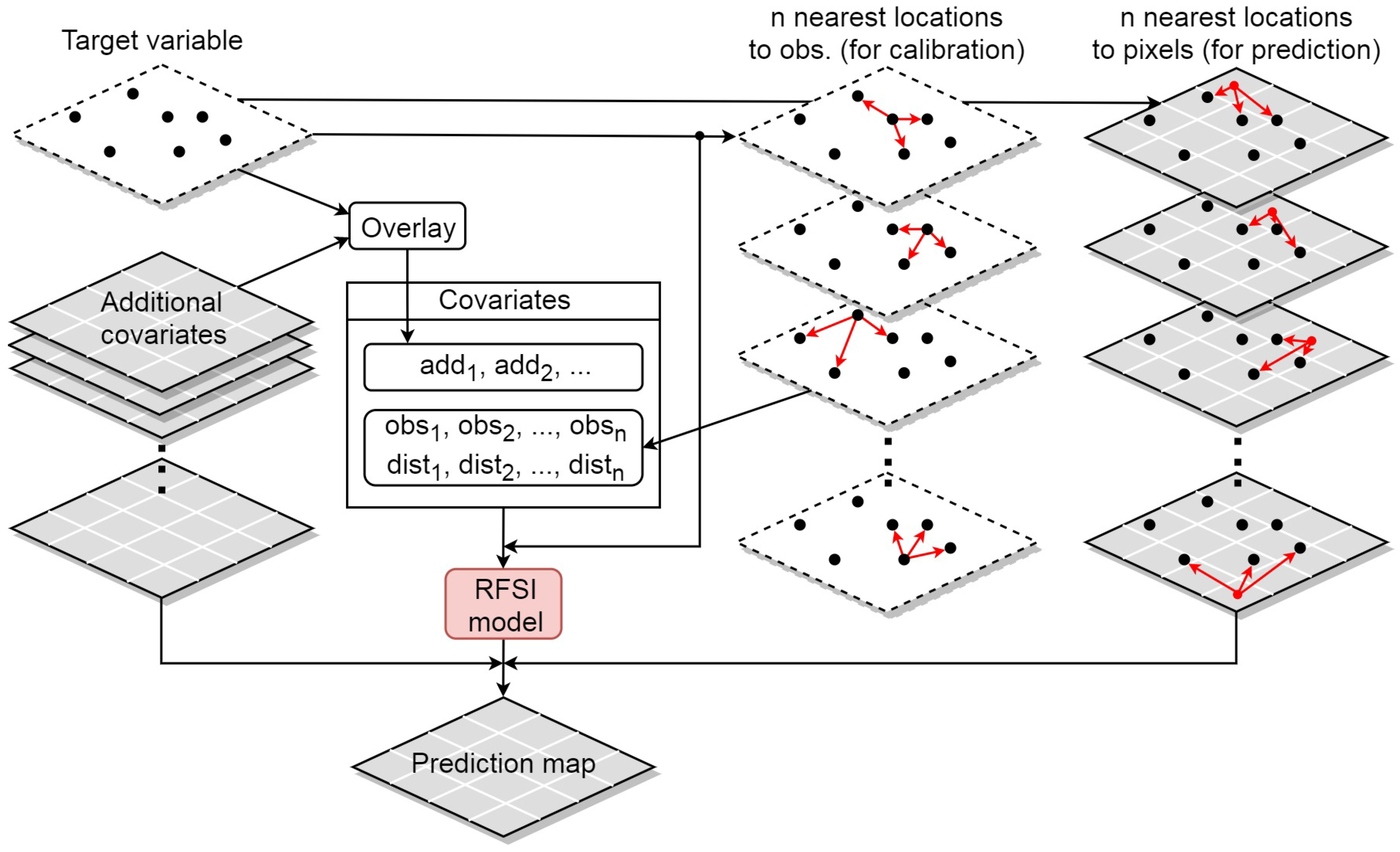
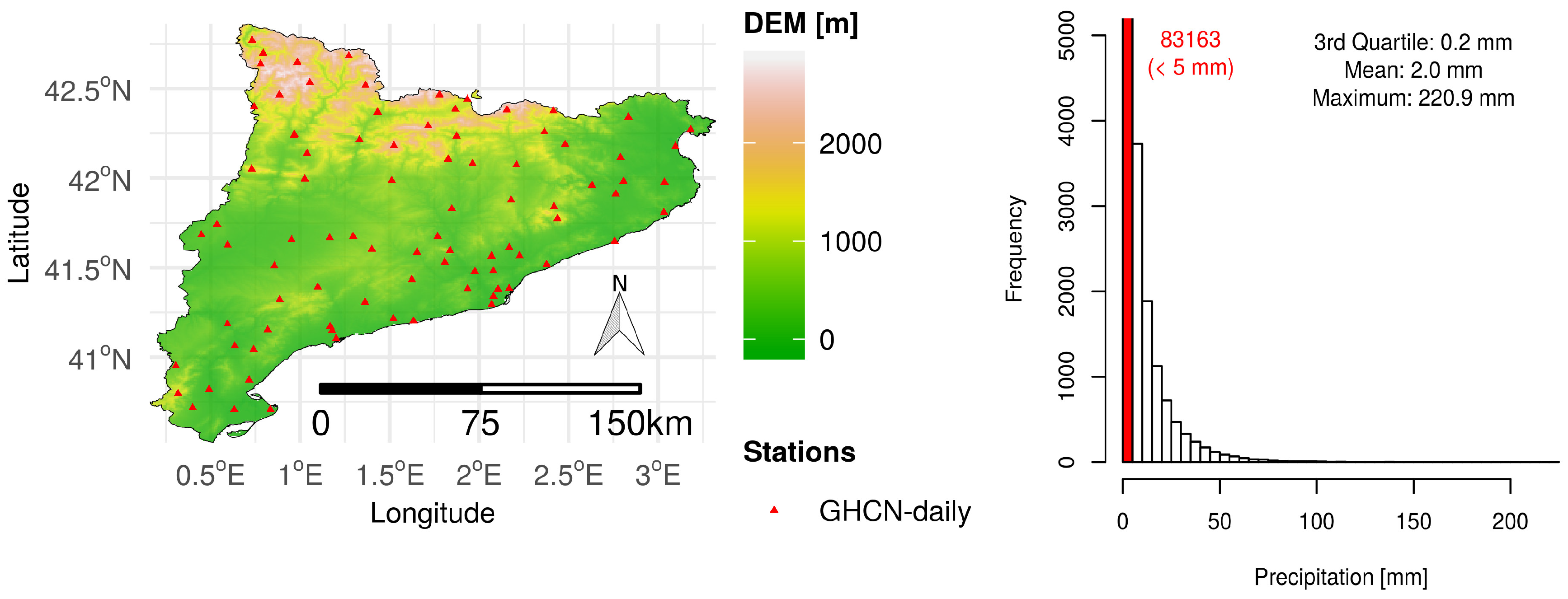
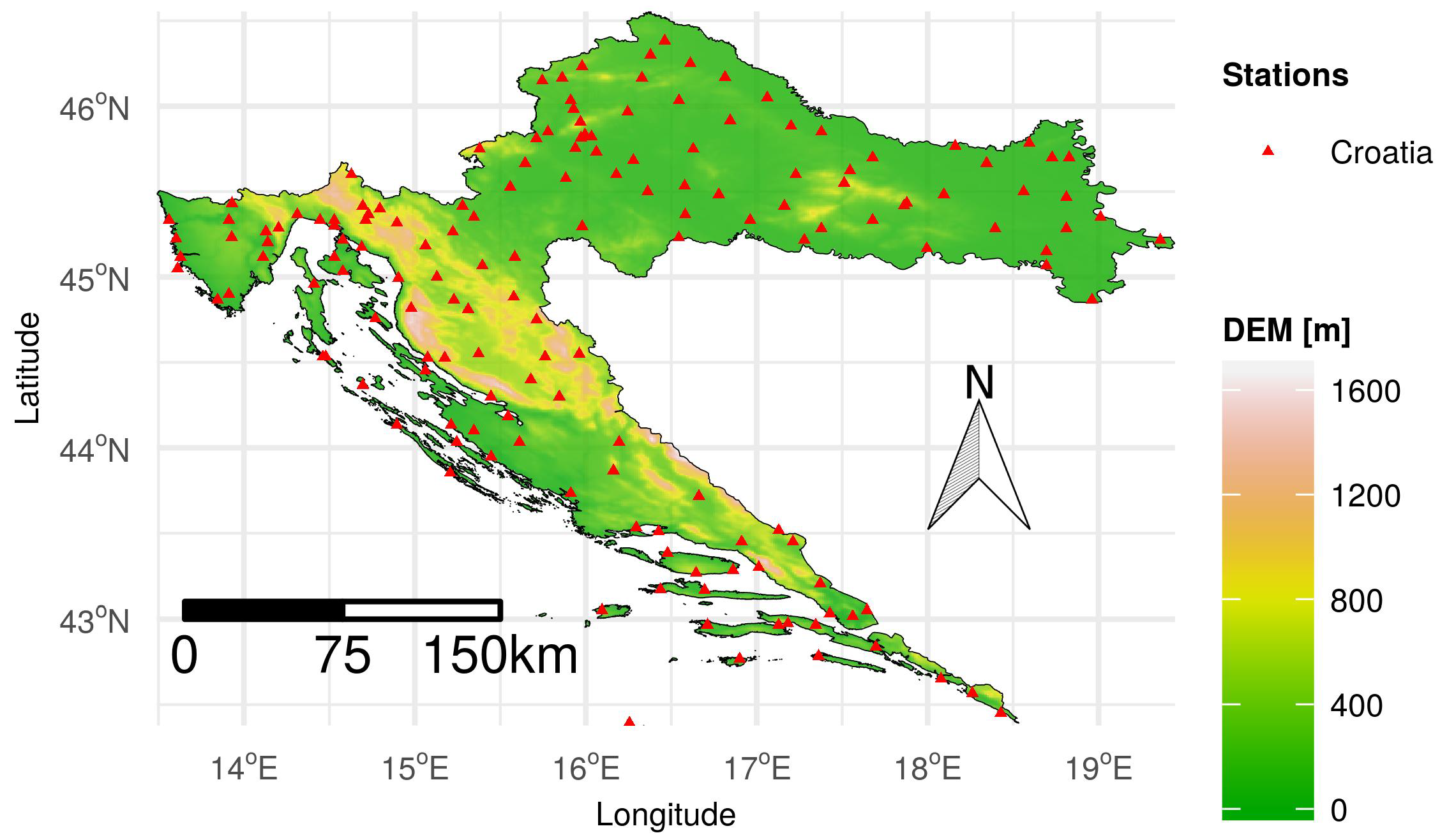
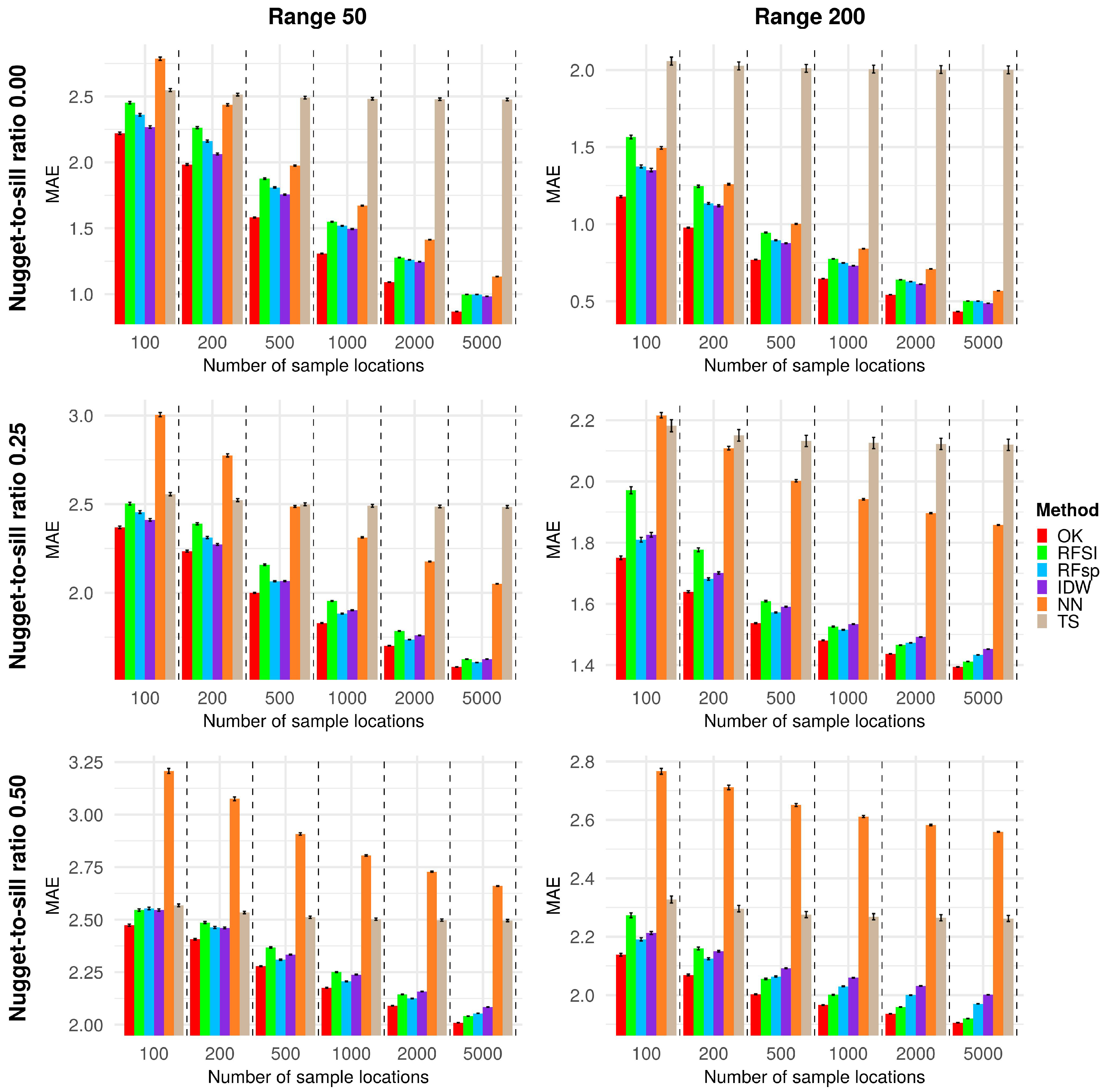
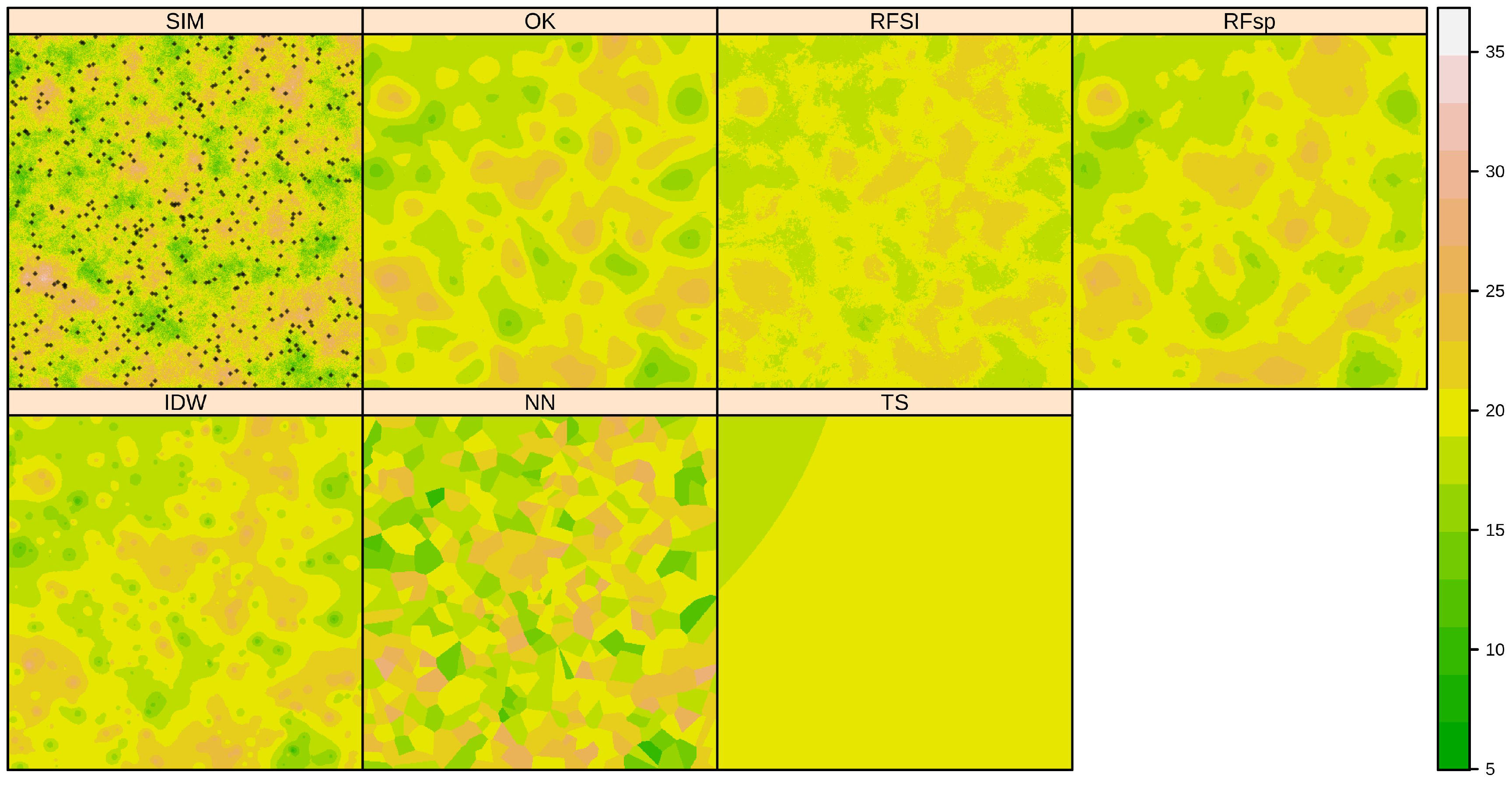
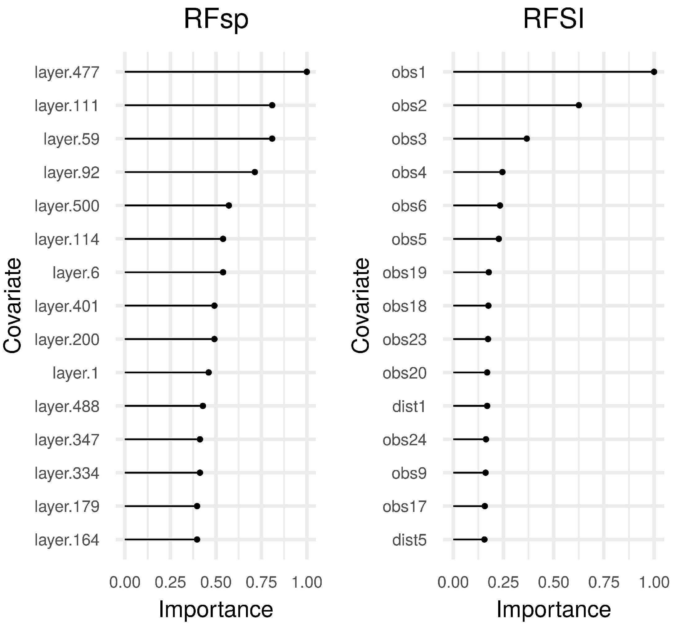
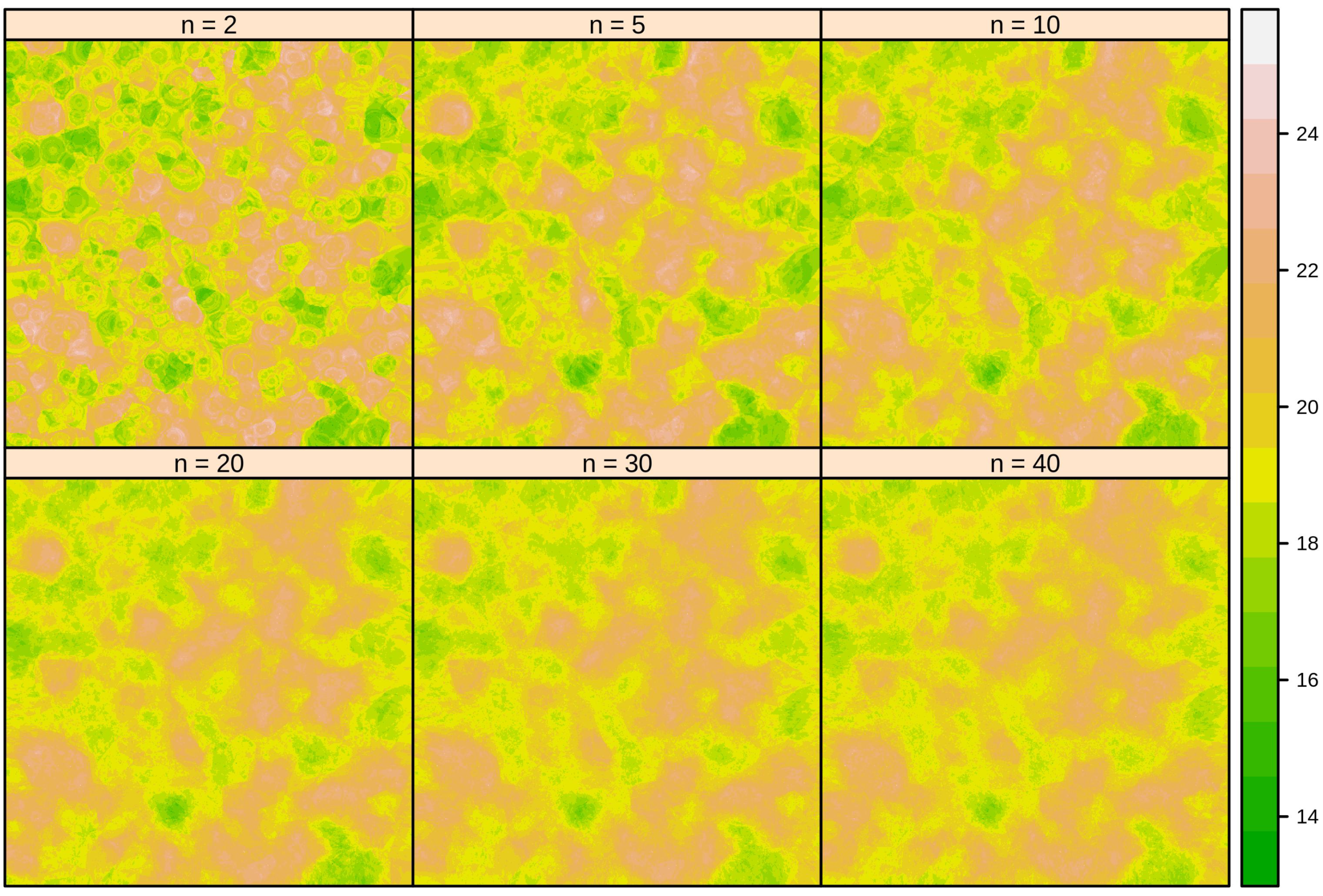
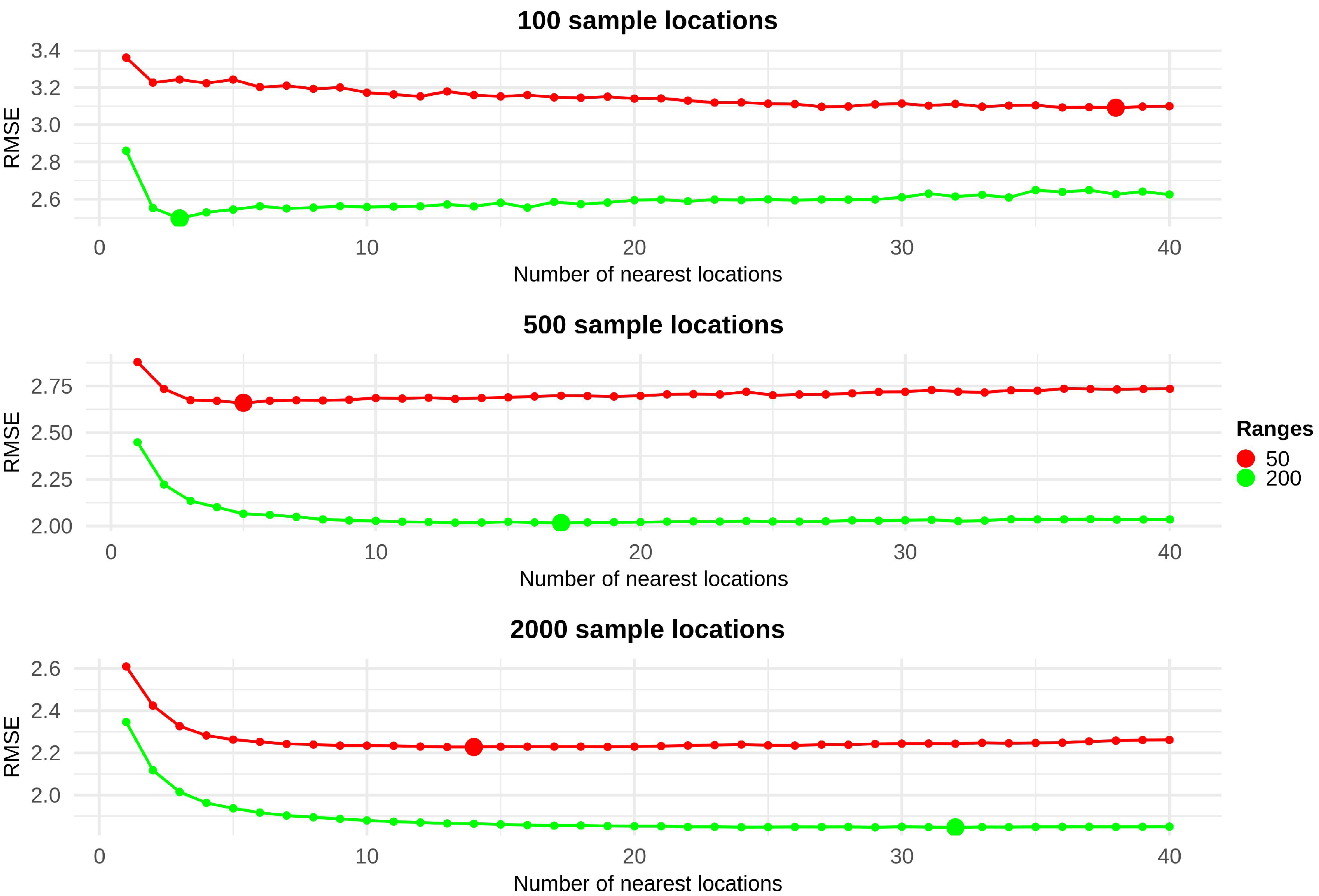
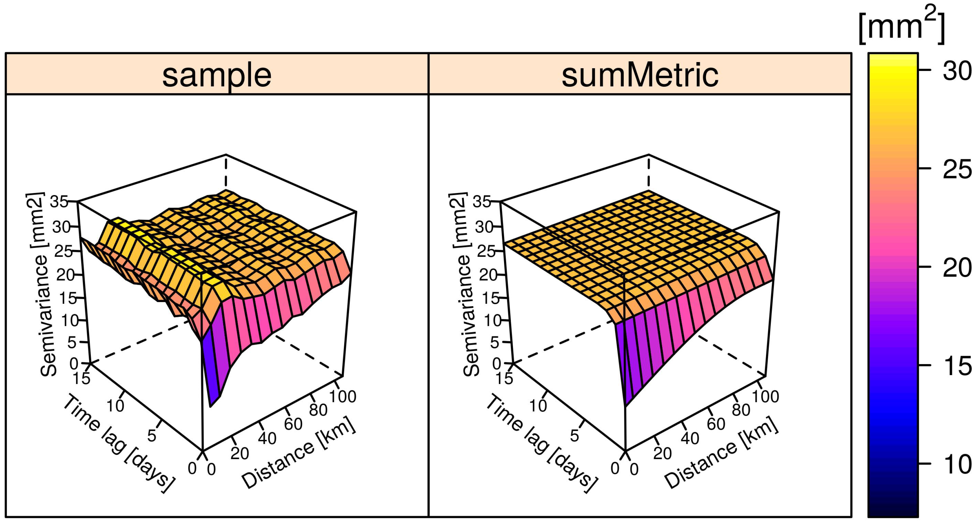
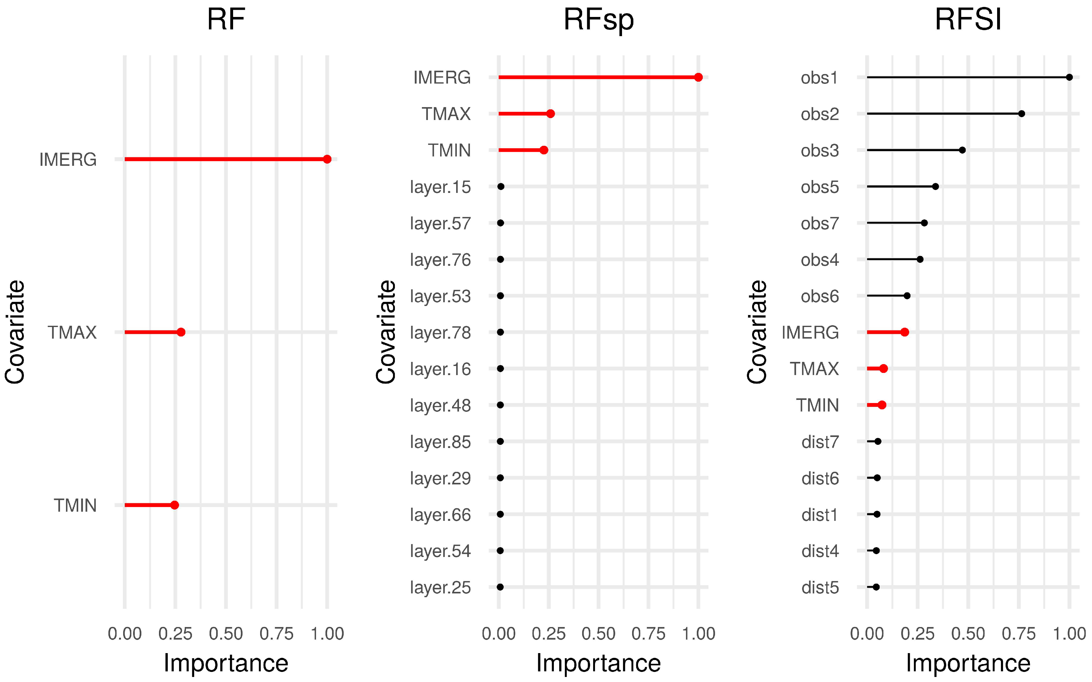
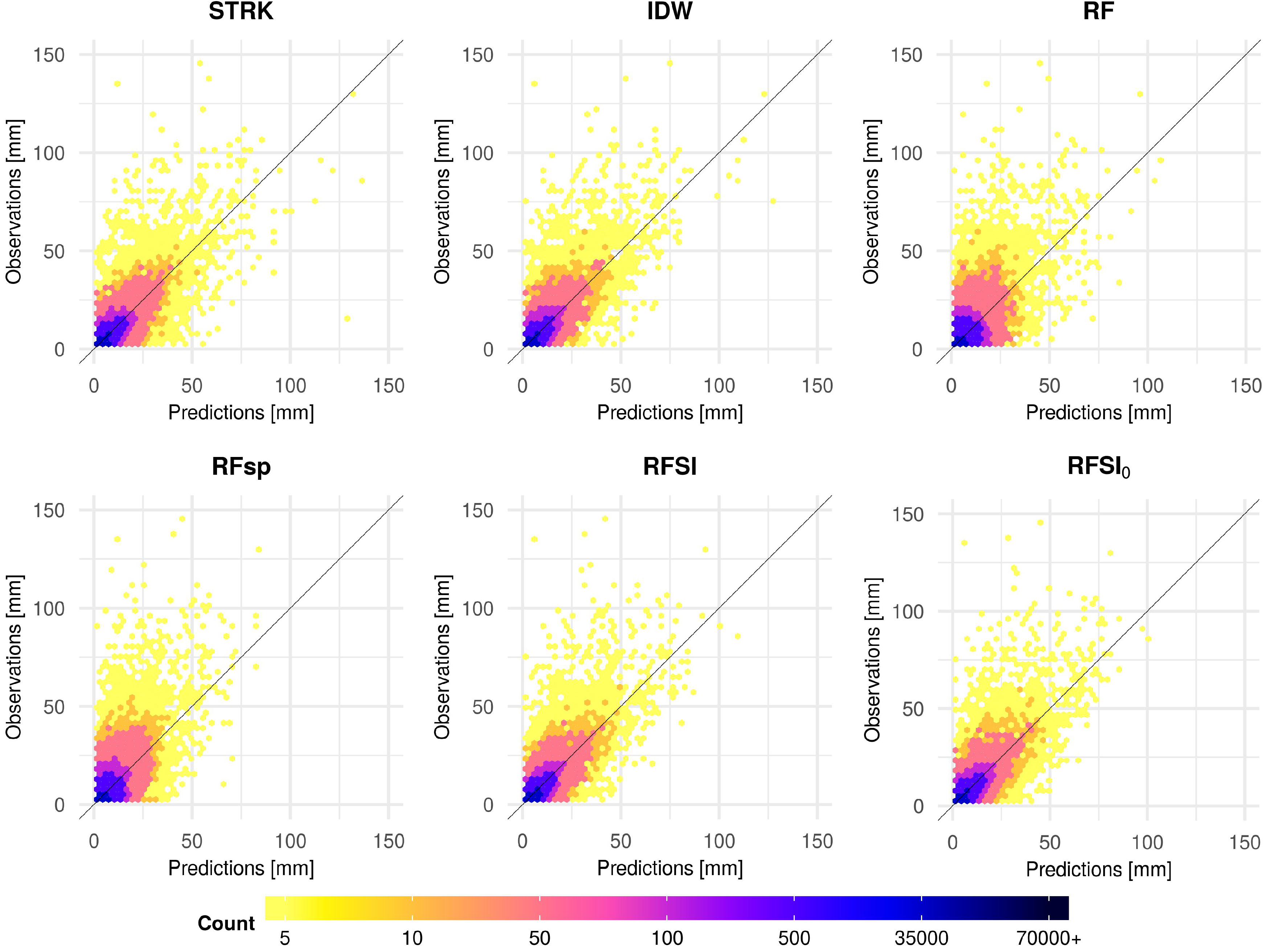
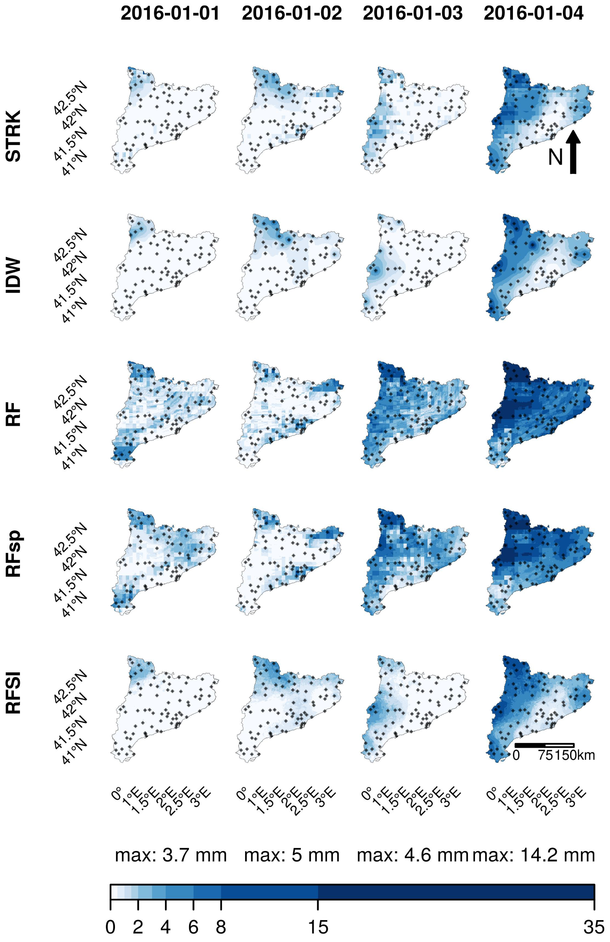
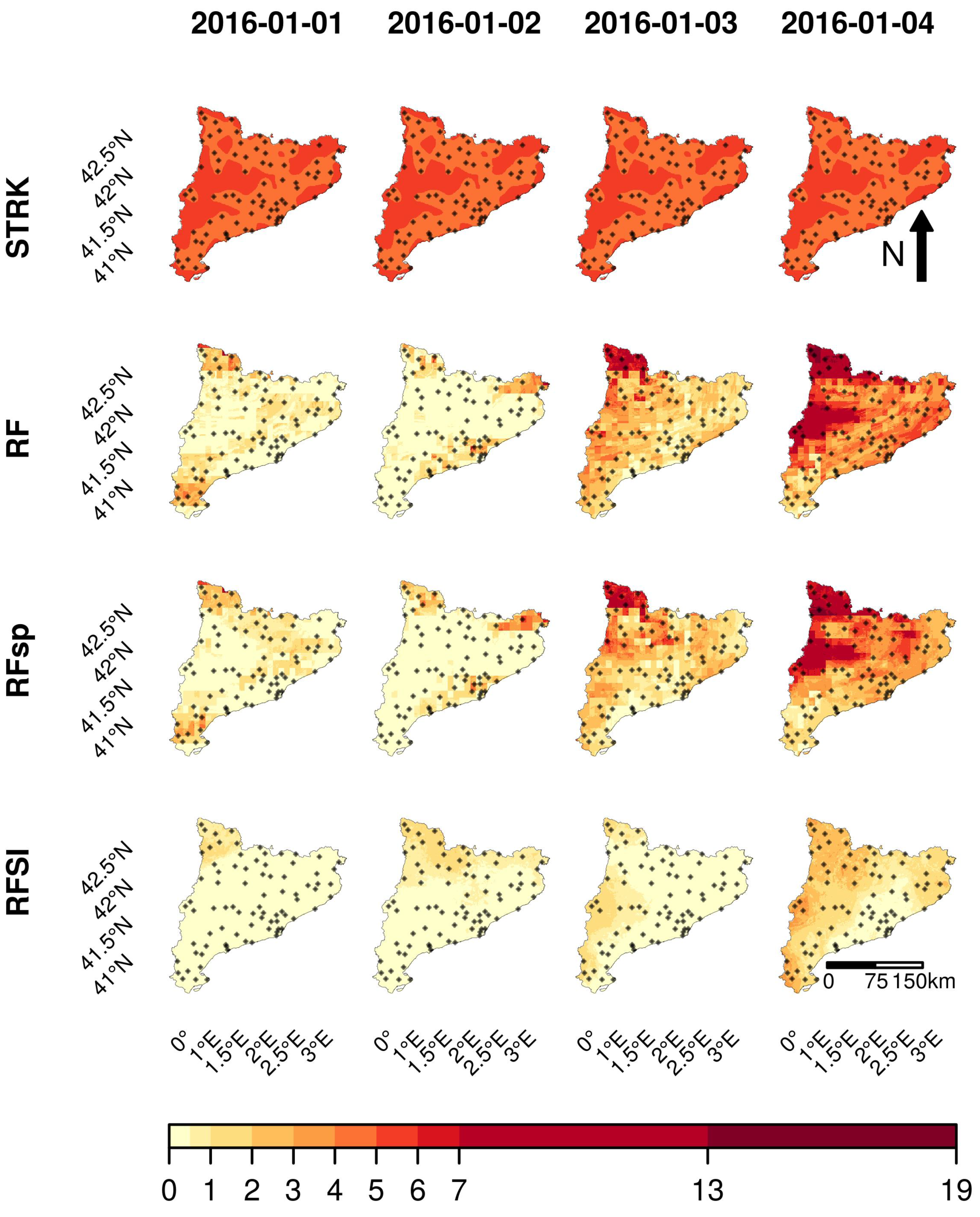
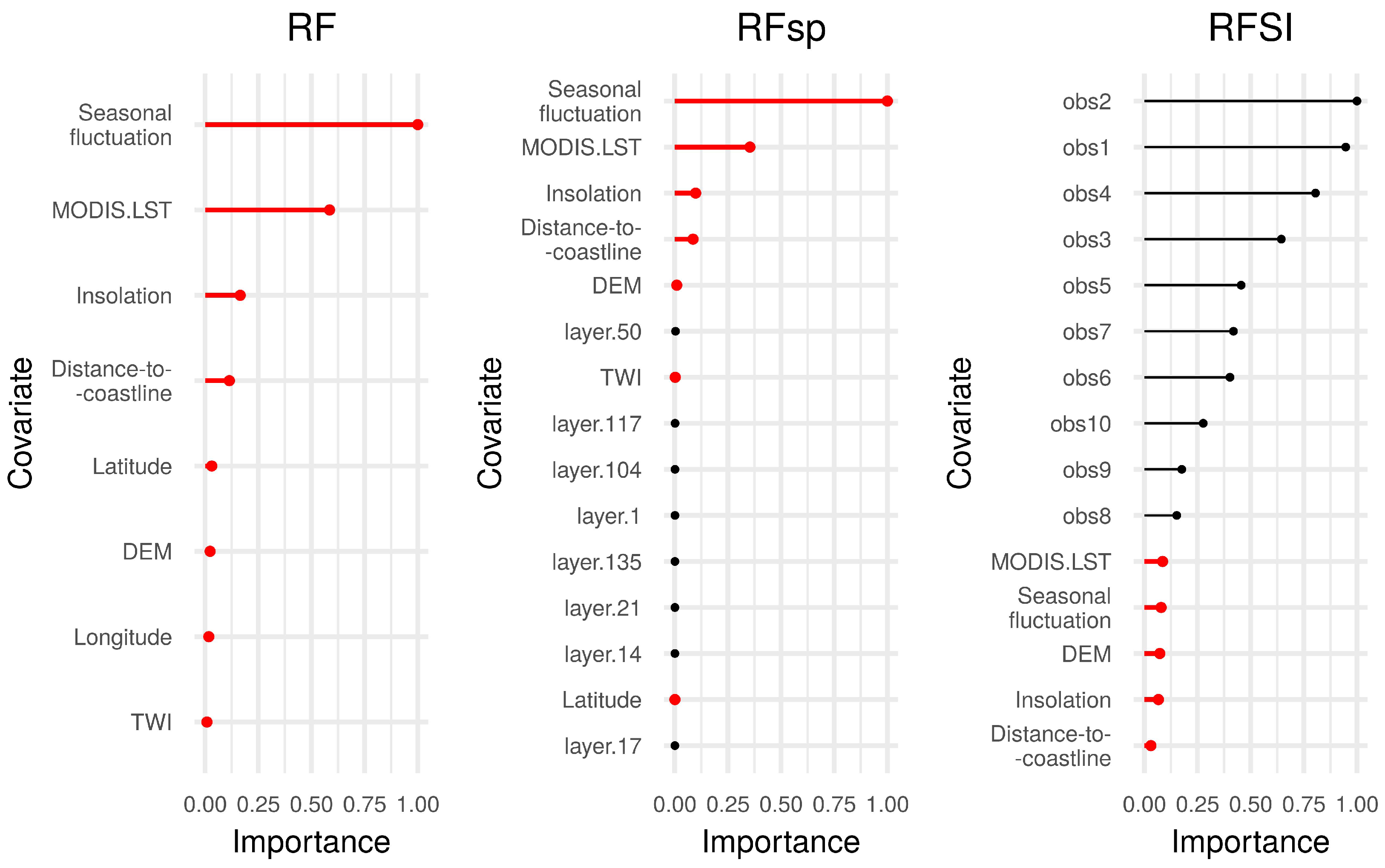
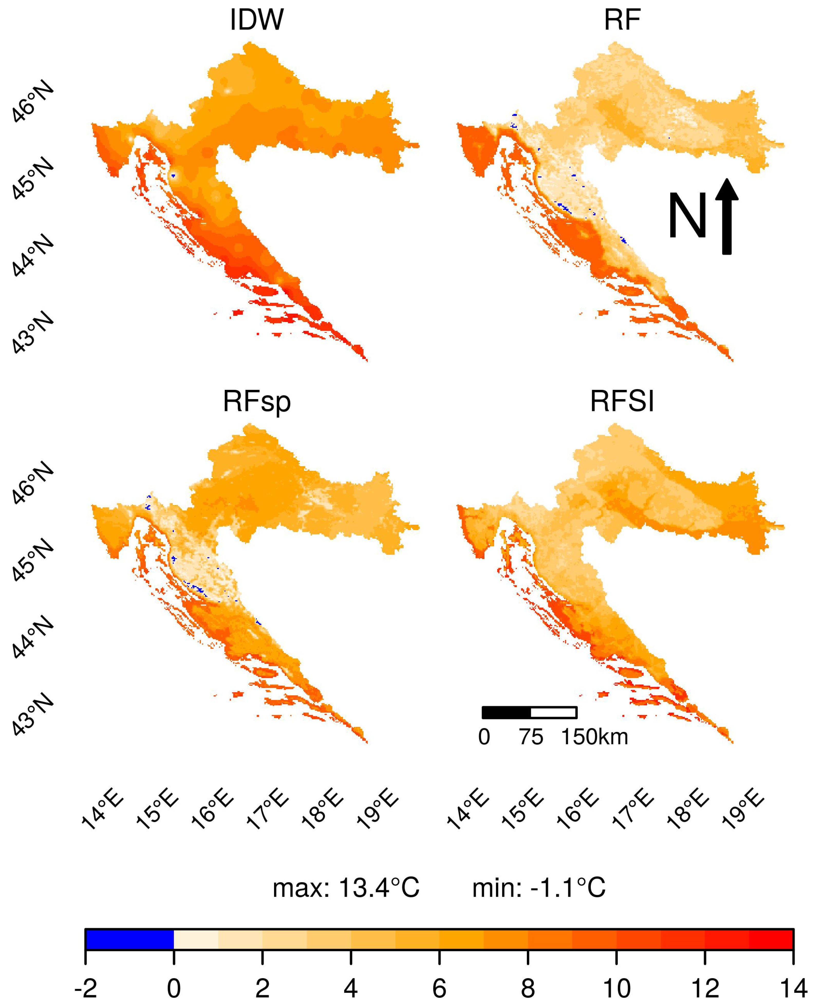
Table 1.
Distance calculation time and modelling time for RFSI and RFsp, and prediction time for RFSI, RFsp and OK. All results refer to the synthetic case study and represent the average computing time computed from 100 simulations. All calculations and time estimations were done on a personal computer with Intel® Core™ i7-7820X CPU @ 3.60GHz × 16 processor and 126 GB of RAM.
| Criteria | Method | Number of Points | |||||
|---|---|---|---|---|---|---|---|
| 100 | 200 | 500 | 1000 | 2000 | 5000 | ||
| Distance calculation time [s] | RFsp | 24.98 | 47.75 | 114.42 | 263.08 | 477.37 | 3832.88 |
| RFSI | 1.40 | 1.48 | 1.62 | 1.65 | 1.69 | 1.75 | |
| Modelling time [s] | RFsp | 0.06 | 0.27 | 2.35 | 13.50 | 71.73 | 498.21 |
| RFSI | 0.02 | 0.04 | 0.09 | 0.20 | 0.42 | 1.18 | |
| Prediction time [s] | OK | 5.25 | 5.72 | 6.38 | 6.81 | 7.11 | 8.03 |
| RFsp | 5.47 | 9.57 | 22.30 | 46.32 | 70.58 | 312.12 | |
| RFSI | 2.93 | 3.37 | 4.05 | 4.74 | 5.60 | 6.83 | |
Table 2.
Sum-metric semivariogram parameters of the STRK model.
| Component | Nugget [mm2] | Sill [mm2] | Range | Function | Anisotropy Ratio |
|---|---|---|---|---|---|
| Spatial | 0.00 | 0.89 | 218.8 km | Spherical | n/a |
| Temporal | 1.63 | 4.15 | 2.6 days | Spherical | n/a |
| Spatio-temporal | 9.51 | 11.30 | 91.7 km | Spherical | 120 km/day |
Table 3.
Optimized hyperparameters of IDW, RF, RFsp and RFSI for the precipitation case study.
| Model | Mtry | Min.Node.Size | Sample.Fraction | n | p |
|---|---|---|---|---|---|
| IDW | n/a | n/a | n/a | 13 | 2.2 |
| RF | 2 | 20 | 0.65 | n/a | n/a |
| RFsp | 58 | 4 | 0.29 | n/a | n/a |
| RFSI | 4 | 6 | 0.95 | 7 | n/a |
Table 4.
Accuracy metrics of all six prediction methods as assessed using nested 5-fold LLOCV for the precipitation case study.
Table 4.
Accuracy metrics of all six prediction methods as assessed using nested 5-fold LLOCV for the precipitation case study.
| Method | R [%] | CCC | MAE [mm] | RMSE [mm] |
|---|---|---|---|---|
| STRK | 67.5 | 0.815 | 1.2 | 3.9 |
| IDW | 69.6 | 0.820 | 1.1 | 3.8 |
| RF | 49.4 | 0.674 | 1.7 | 4.9 |
| RFsp | 53.3 | 0.690 | 1.6 | 4.7 |
| RFSI | 69.5 | 0.820 | 1.1 | 3.8 |
| RFSI | 68.6 | 0.814 | 1.2 | 3.9 |
Table 5.
Performance of all models for precipitation below and above 1 mm. Values for the hits and misses are number of observations (obs.) for a given condition. Predictions (pred.) used in this table are from nested 5-fold LLOCV. Overall accuracy represents the percentage of correct classifications. Numbers in bold represent the best performance.
| Hits | Misses | RMSE [mm] | Overall | |||||
|---|---|---|---|---|---|---|---|---|
| Method | obs. pred. | < 1 mm < 1 mm | ≥ 1 mm ≥ 1 mm | < 1 mm ≥ 1 mm | ≥ 1 mm < 1 mm | < 1 mm | ≥ 1 mm | Accuracy [%] |
| STRK | 68,272 | 15,894 | 6307 | 1847 | 1.2 | 8.6 | 91.2 | |
| IDW | 68,398 | 16,164 | 6181 | 1577 | 1.0 | 8.4 | 91.6 | |
| RF | 63,382 | 14,914 | 11,197 | 2827 | 1.7 | 10.6 | 84.8 | |
| RFsp | 64,235 | 15,273 | 10,344 | 2468 | 1.6 | 10.2 | 86.1 | |
| RFSI | 68,031 | 16,524 | 6548 | 1217 | 1.0 | 8.4 | 91.6 | |
| RFSI | 67,917 | 16,535 | 6662 | 1206 | 1.0 | 8.5 | 91.5 | |
Table 6.
Optimized hyperparameters of IDW, RF, RFsp, and RFSI for the temperature case study.
| Model | Mtry | Min.Node.Size | Sample.Fraction | n | p |
|---|---|---|---|---|---|
| IDW | n/a | n/a | n/a | 11 | 1.8 |
| RF | 6 | 3 | 0.85 | n/a | n/a |
| RFsp | 154 | 2 | 0.77 | n/a | n/a |
| RFSI | 5 | 15 | 0.90 | 10 | n/a |
Table 7.
Accuracy metrics of all six prediction methods as assessed using nested 10-fold LLOCV for the temperature case study. Note that accuracy metrics for STRK are taken from Hengl et al. [26].
Table 7.
Accuracy metrics of all six prediction methods as assessed using nested 10-fold LLOCV for the temperature case study. Note that accuracy metrics for STRK are taken from Hengl et al. [26].
| Method | R [%] | CCC | MAE [mm] | RMSE [mm] |
|---|---|---|---|---|
| STRK | 91.0 | n/a | n/a | 2.4 |
| IDW | 95.0 | 0.974 | 1.2 | 1.8 |
| RF | 95.7 | 0.978 | 1.1 | 1.6 |
| RFsp | 95.5 | 0.976 | 1.1 | 1.6 |
| RFSI | 96.6 | 0.983 | 1.0 | 1.4 |
| RFSI | 94.9 | 0.974 | 1.2 | 1.8 |
© 2020 by the authors. Licensee MDPI, Basel, Switzerland. This article is an open access article distributed under the terms and conditions of the Creative Commons Attribution (CC BY) license (http://creativecommons.org/licenses/by/4.0/).
Share and Cite
MDPI and ACS Style
Sekulić, A.; Kilibarda, M.; Heuvelink, G.B.M.; Nikolić, M.; Bajat, B. Random Forest Spatial Interpolation. Remote Sens. 2020, 12, 1687. https://doi.org/10.3390/rs12101687
AMA Style
Sekulić A, Kilibarda M, Heuvelink GBM, Nikolić M, Bajat B. Random Forest Spatial Interpolation. Remote Sensing. 2020; 12(10):1687. https://doi.org/10.3390/rs12101687
Chicago/Turabian StyleSekulić, Aleksandar, Milan Kilibarda, Gerard B.M. Heuvelink, Mladen Nikolić, and Branislav Bajat. 2020. "Random Forest Spatial Interpolation" Remote Sensing 12, no. 10: 1687. https://doi.org/10.3390/rs12101687
Note that from the first issue of 2016, this journal uses article numbers instead of page numbers. See further details here.