Robust Visual-Inertial Integrated Navigation System Aided by Online Sensor Model Adaption for Autonomous Ground Vehicles in Urban Areas


Abstract
1. Introduction
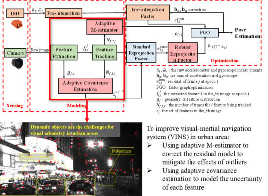
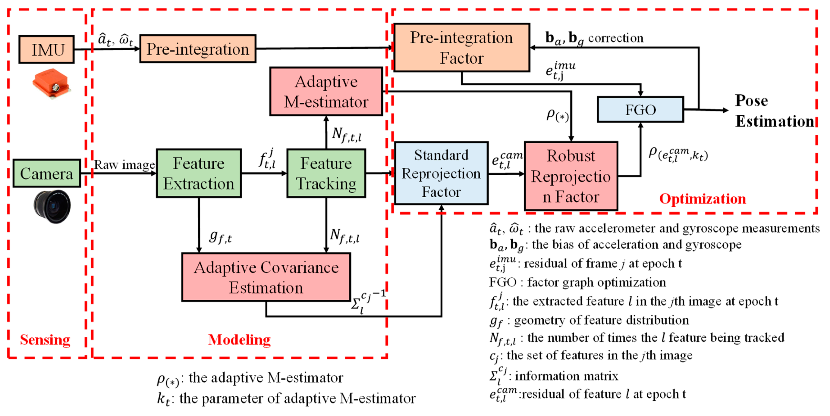
2. Overview of the Proposed Adaptive VINS
- (1)
- This study proposes a self-tuning covariance estimation approach to model the uncertainty of each feature measurement by integrating two parts: (1) the geometry of feature distribution (GFD); (2) the quality of feature tracking;
- (2)
- This study proposes an adaptive M-estimator to correct the measurement residual model to further mitigate the effects of outlier measurements, like the dynamic features. The proposed adaptive M-estimator effectively relaxed the drawback of manual parameterization [36] of M-estimator;
- (3)
- This study employs challenging datasets collected in dynamic urban canyons of Hong Kong to validate the effectiveness of the proposed method in mitigating the effects of dynamic objects. improved performance is achieved compared with the state-of-the-art VINS solution [6].
3. Tightly Coupled Monocular-based Visual-inertial Integration based on Factor Graph Optimization
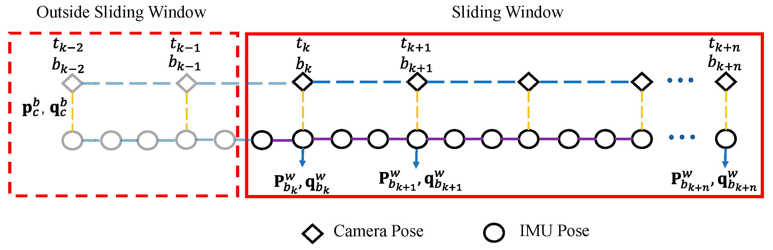
3.1. System States
3.2. IMU Measurement Modeling
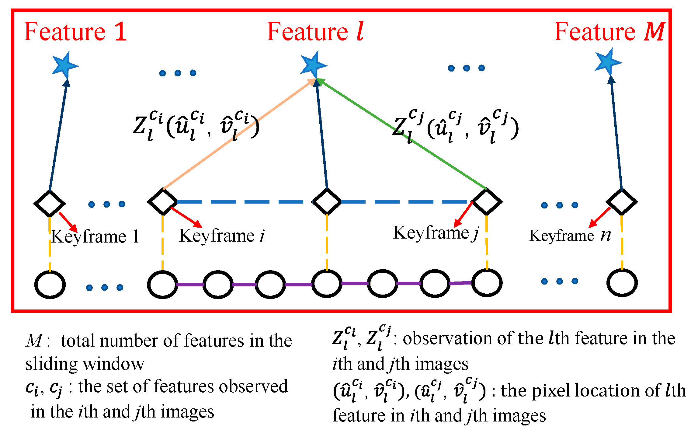
3.3. Visual Measurement Modeling
3.4. Marginalization
3.5. Visual-Inertia Optimization
4. Online Sensor Model Estimation
4.1. Adaptive Covariance Estimation
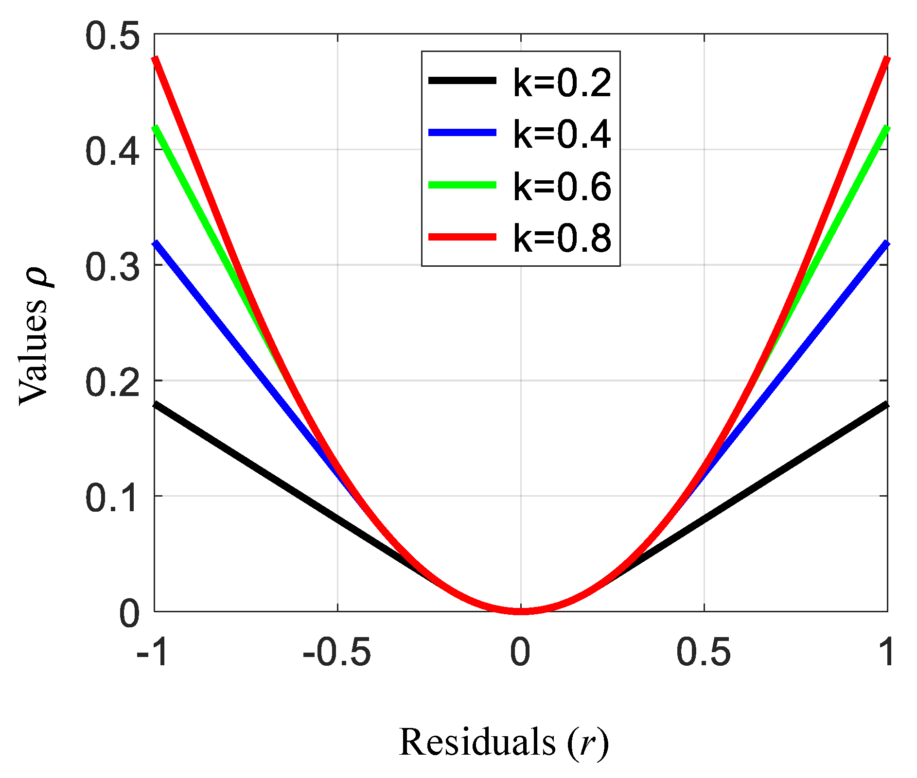
4.2. Adaptive M-Estimator
4.3. Visual-Inertia Optimization with Online Sensor Model
5. Experimental Results
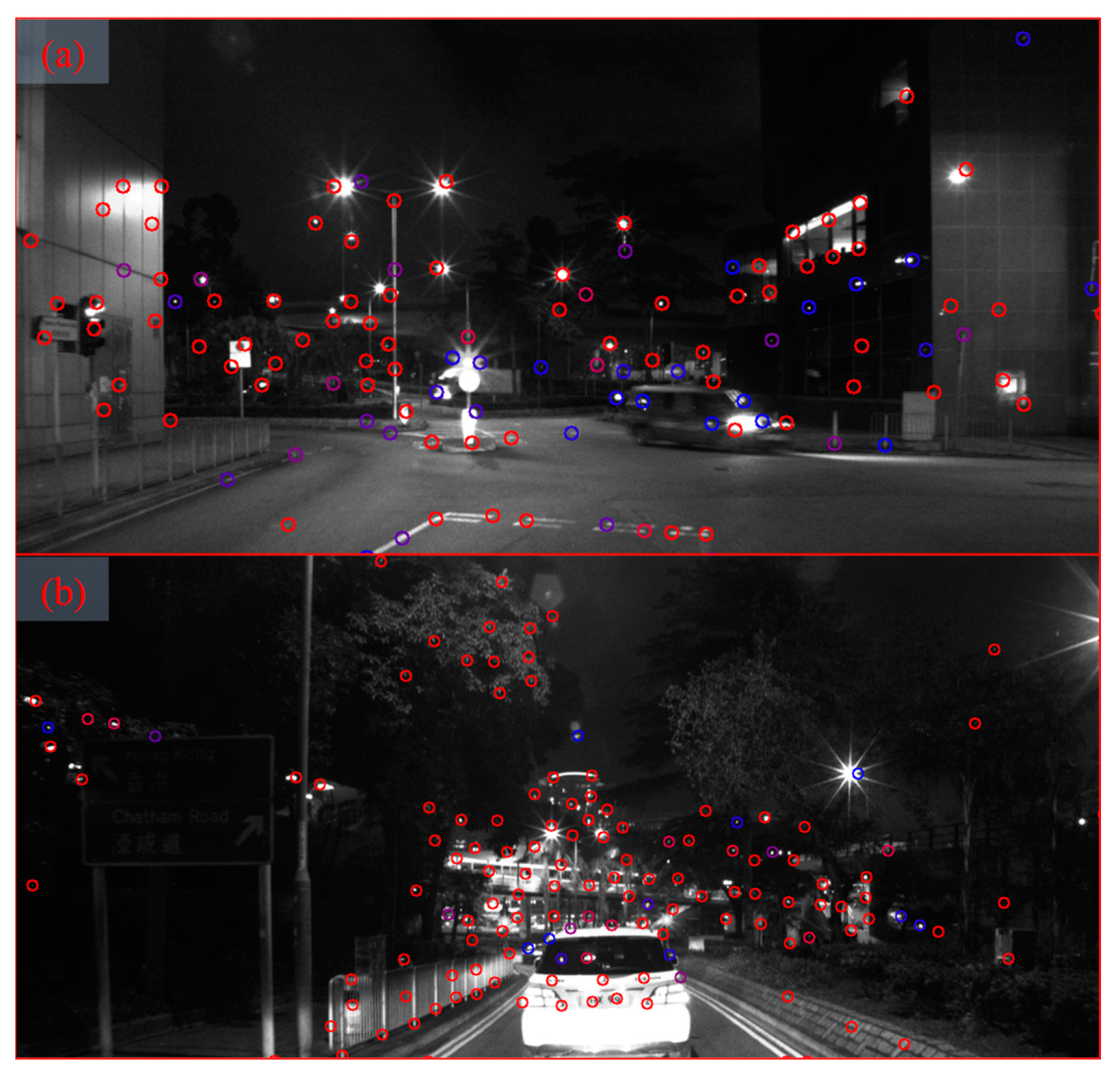
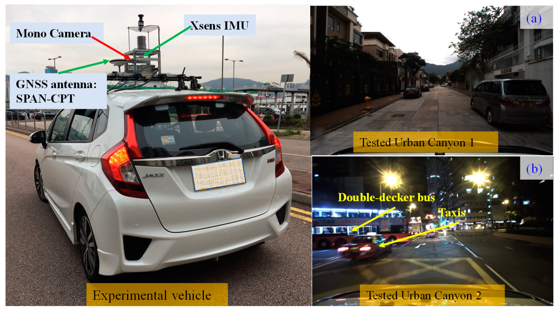
5.1. Experimental Setup
- (1)
- VINS: the original VINS solution from [6].
- (2)
- VINS–AC: VINS-aided by adaptive covariance estimation proposed in Section 4.1.
- VINS-Adaptive covariance (): only consider during covariance estimation
- VINS-Adaptive covariance (): consider both and during covariance estimation.
- (3)
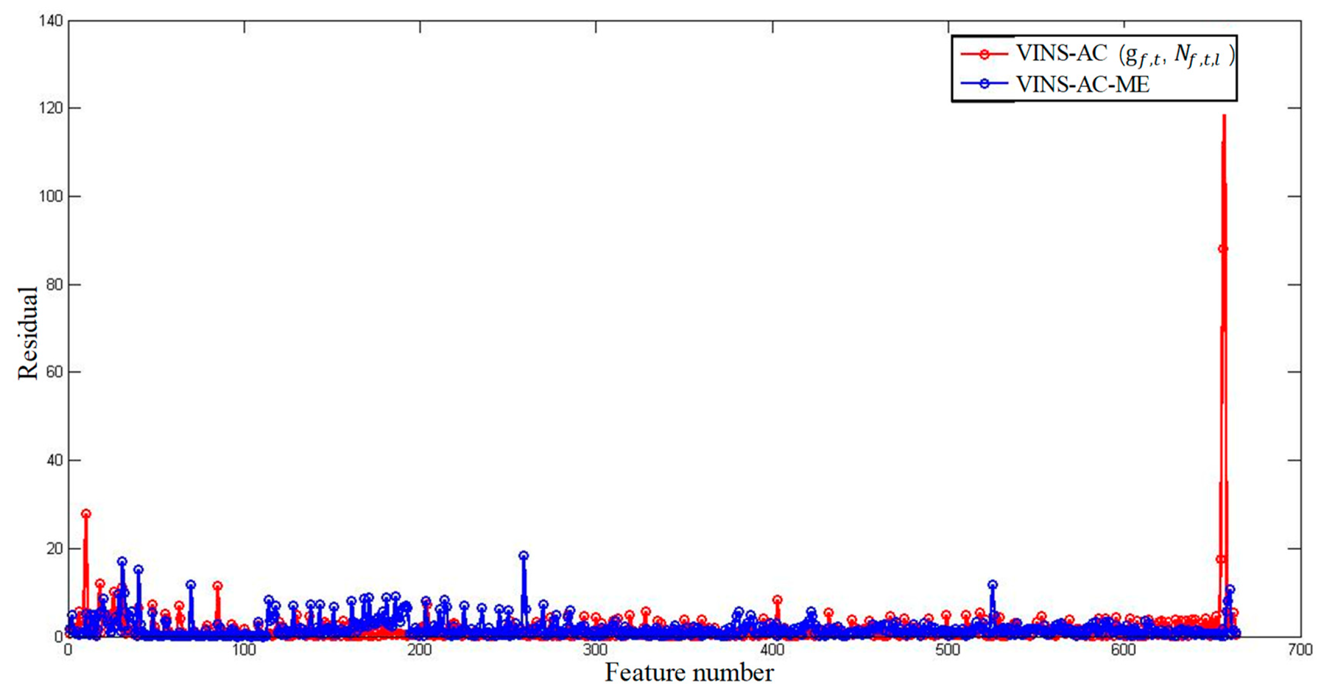
- VINS–AC–ME: VINS-aided by adaptive covariance estimation proposed in Section 4.1 and adaptive M-estimator in Section 4.2.
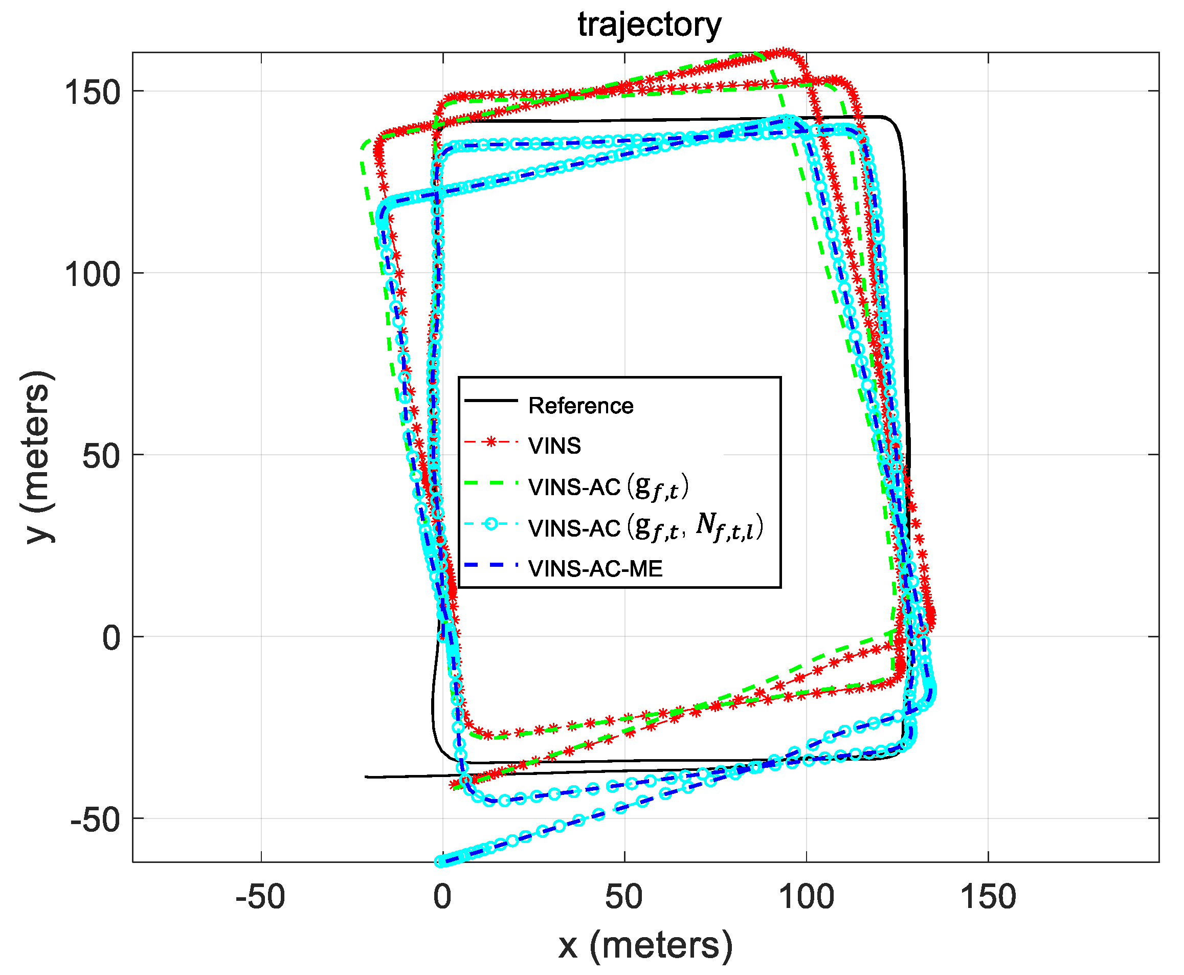
5.2. Evaluation of the Dataset Collected in Urban Canyon 1
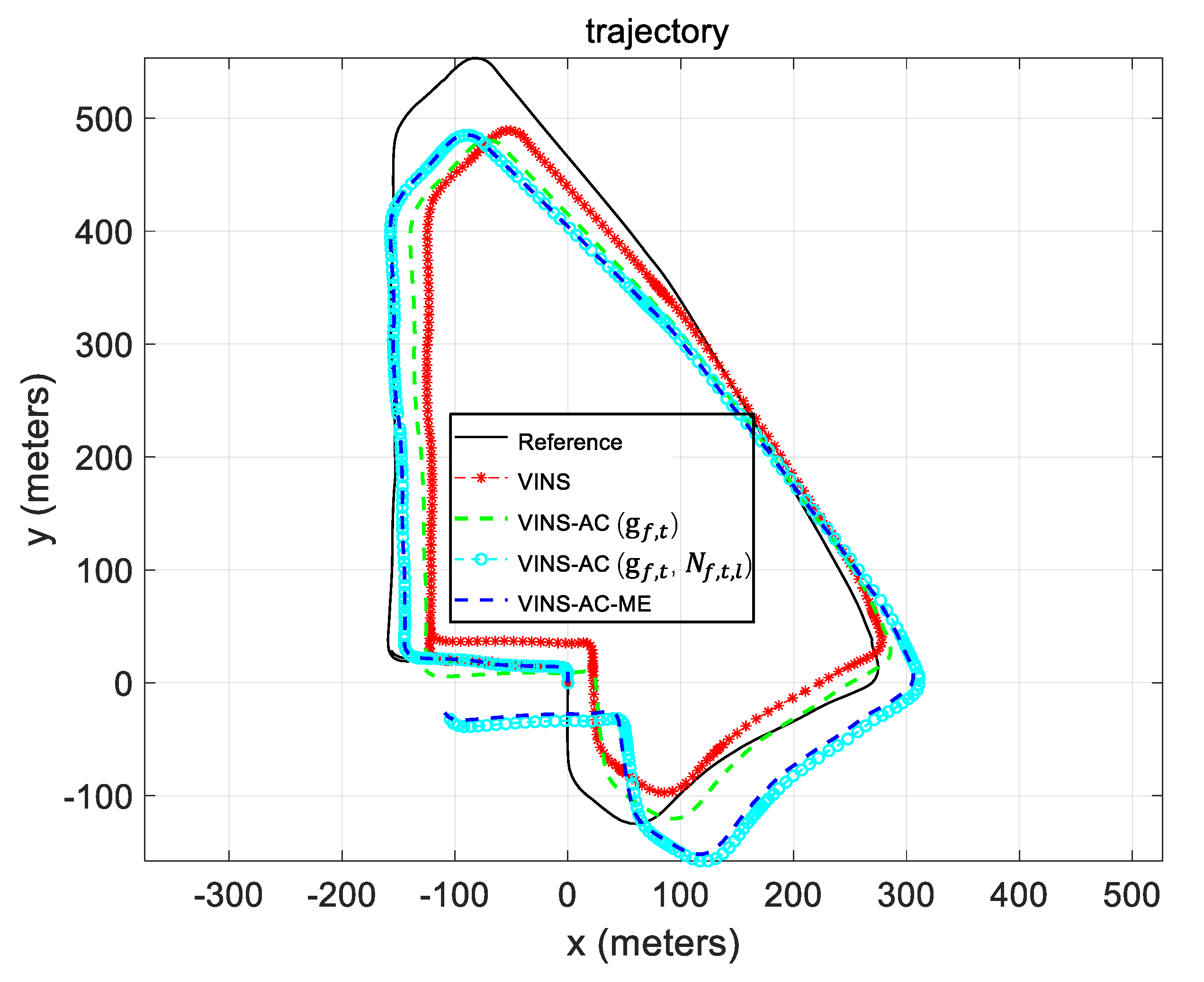
5.3. Evaluation of the Data Collected in Urban Canyon 2
6. Conclusions and Future Work
Author Contributions
Funding
Conflicts of Interest
References
- Bloesch, M.; Omari, S.; Hutter, M.; Siegwart, R. Robust visual inertial odometry using a direct EKF-based approach. In Proceedings of the 2015 IEEE/RSJ International Conference on Intelligent Robots and Systems (IROS), Hamburg, Germany, 28 September–2 October 2015; pp. 298–304. [Google Scholar]
- Li, R.; Liu, J.; Zhang, L.; Hang, Y. LIDAR/MEMS IMU integrated navigation (SLAM) method for a small UAV in indoor environments. In Proceedings of the 2014 DGON Inertial Sensors and Systems (ISS), Karlsruhe, Germany, 16–17 September 2014; pp. 1–15. [Google Scholar]
- Siegl, H.; Pinz, A. A mobile AR kit as a human computer interface for cognitive vision. In Proceedings of the 5th International Workshop on Image Analysis for Multimedia Interactive Services, WIAMIS, Lisboa, Portugal, 21–23 April 2004. [Google Scholar]
- Qin, T.; Pan, J.; Cao, S.; Shen, S. A general optimization-based framework for local odometry estimation with multiple sensors. arXiv 2019, arXiv:1901.03638. [Google Scholar]
- Pfrommer, B.; Sanket, N.; Daniilidis, K.; Cleveland, J. Penncosyvio: A challenging visual inertial odometry benchmark. In Proceedings of the 2017 IEEE International Conference on Robotics and Automation (ICRA), Singapore, 29 May–3 June 2017; pp. 3847–3854. [Google Scholar]
- Qin, T.; Li, P.; Shen, S. Vins-mono: A robust and versatile monocular visual-inertial state estimator. IEEE Trans. Robot. 2018, 34, 1004–1020. [Google Scholar] [CrossRef]
- Von Stumberg, L.; Usenko, V.; Cremers, D. Direct sparse visual-inertial odometry using dynamic marginalization. In Proceedings of the 2018 IEEE International Conference on Robotics and Automation (ICRA), Brisbane, Australia, 21–25 May 2018; pp. 2510–2517. [Google Scholar]
- Xu, W.; Choi, D.; Wang, G. Direct visual-inertial odometry with semi-dense mapping. Comput. Electr. Eng. 2018, 67, 761–775. [Google Scholar] [CrossRef]
- Rebecq, H.; Horstschaefer, T.; Scaramuzza, D. Real-time Visual-Inertial Odometry for Event Cameras using Keyframe-based Nonlinear Optimization. In Proceedings of the BMVC, London, UK, 4–7 September 2017. [Google Scholar]
- Saputra, M.R.U.; Markham, A.; Trigoni, N. Visual SLAM and structure from motion in dynamic environments: A survey. ACM Comput. Surv. (CSUR) 2018, 51, 37. [Google Scholar] [CrossRef]
- Bai, X.; Wen, W.; Hsu, L.-T. Performance Analysis of Visual/Inertial Integrated Positioning in Diverse Typical Urban Scenarios of Hong Kong. In Proceedings of the Asian-Pacific Conference on Aerospace Technology and Science, Taiwan, 28–31 August 2019. [Google Scholar]
- Yazdi, M.; Bouwmans, T. New trends on moving object detection in video images captured by a moving camera: A survey. Comput. Sci. Rev. 2018, 28, 157–177. [Google Scholar] [CrossRef]
- Mane, S.; Mangale, S. Moving Object Detection and Tracking Using Convolutional Neural Networks. In Proceedings of the 2018 Second International Conference on Intelligent Computing and Control Systems (ICICCS), Madurai, India, 14–15 June 2018; pp. 1809–1813. [Google Scholar]
- Sun, Y.; Liu, M.; Meng, M.Q.-H. Improving RGB-D SLAM in dynamic environments: A motion removal approach. Robot. Auton. Syst. 2017, 89, 110–122. [Google Scholar] [CrossRef]
- Sun, Y.; Liu, M.; Meng, M.Q.-H. Motion removal for reliable RGB-D SLAM in dynamic environments. Robot. Auton. Syst. 2018, 108, 115–128. [Google Scholar] [CrossRef]
- Wang, Y.; Huang, S. Motion segmentation based robust RGB-D SLAM. In Proceedings of the 11th World Congress on Intelligent Control and Automation, Shenyang, China, 29 June–4 July 2014; pp. 3122–3127. [Google Scholar]
- Herbst, E.; Ren, X.; Fox, D. Rgb-d flow: Dense 3-d motion estimation using color and depth. In Proceedings of the 2013 IEEE International Conference on Robotics and Automation, Karlsruhe, Germany, 6–10 May 2013; pp. 2276–2282. [Google Scholar]
- Mur-Artal, R.; Tardós, J.D. Orb-slam2: An open-source slam system for monocular, stereo, and rgb-d cameras. IEEE Trans. Robot. 2017, 33, 1255–1262. [Google Scholar] [CrossRef]
- Endres, F.; Hess, J.; Engelhard, N.; Sturm, J.; Cremers, D.; Burgard, W. An evaluation of the RGB-D SLAM system. In Proceedings of the ICRA, Saint Paul, MN, USA, 14–18 May 2012; pp. 1691–1696. [Google Scholar]
- Yamaguchi, K.; Kato, T.; Ninomiya, Y. Vehicle ego-motion estimation and moving object detection using a monocular camera. In Proceedings of the 18th International Conference on Pattern Recognition (ICPR’06), Hong Kong, China, 20–24 August 2006; pp. 610–613. [Google Scholar]
- Zhou, D.; Frémont, V.; Quost, B.; Wang, B. On modeling ego-motion uncertainty for moving object detection from a mobile platform. In Proceedings of the 2014 IEEE Intelligent Vehicles Symposium Proceedings, Dearborn, MI, USA, 8–11 June 2014; pp. 1332–1338. [Google Scholar]
- Milz, S.; Arbeiter, G.; Witt, C.; Abdallah, B.; Yogamani, S. Visual slam for automated driving: Exploring the applications of deep learning. In Proceedings of the IEEE Conference on Computer Vision and Pattern Recognition Workshops, Salt Lake City, UT, USA, 18–22 June 2018; pp. 247–257. [Google Scholar]
- Bahraini, M.S.; Rad, A.B.; Bozorg, M. SLAM in Dynamic Environments: A Deep Learning Approach for Moving Object Tracking Using ML-RANSAC Algorithm. Sensors 2019, 19, 3699. [Google Scholar] [CrossRef]
- Zhong, F.; Wang, S.; Zhang, Z.; Wang, Y. Detect-SLAM: Making object detection and slam mutually beneficial. In Proceedings of the 2018 IEEE Winter Conference on Applications of Computer Vision (WACV), Lake Tahoe, NV, USA, 12–15 March 2018; pp. 1001–1010. [Google Scholar]
- Bescos, B.; Fácil, J.M.; Civera, J.; Neira, J. DynaSLAM: Tracking, mapping, and inpainting in dynamic scenes. IEEE Robot. Autom. Lett. 2018, 3, 4076–4083. [Google Scholar] [CrossRef]
- Xiao, L.; Wang, J.; Qiu, X.; Rong, Z.; Zou, X. Dynamic-SLAM: Semantic monocular visual localization and mapping based on deep learning in dynamic environment. Robot. Auton. Syst. 2019, 117, 1–16. [Google Scholar] [CrossRef]
- Liu, W.; Anguelov, D.; Erhan, D.; Szegedy, C.; Reed, S.; Fu, C.-Y.; Berg, A.C. Ssd: Single shot multibox detector. In Proceedings of the European Conference on Computer Vision, Amsterdam, The Netherlands, 8–16 October 2016; pp. 21–37. [Google Scholar]
- Labbe, M.; Michaud, F. Online global loop closure detection for large-scale multi-session graph-based SLAM. In Proceedings of the 2014 IEEE/RSJ International Conference on Intelligent Robots and Systems, Chicago, IL, USA, 14–18 September 2014; pp. 2661–2666. [Google Scholar]
- Redmon, J.; Divvala, S.; Girshick, R.; Farhadi, A. You only look once: Unified, real-time object detection. In Proceedings of the IEEE Conference on Computer Vision and Pattern Recognition, Las Vegas, NV, USA, 27–30 June 2016; pp. 779–788. [Google Scholar]
- Lin, T.-Y.; Dollár, P.; Girshick, R.; He, K.; Hariharan, B.; Belongie, S. Feature pyramid networks for object detection. In Proceedings of the IEEE Conference on Computer Vision and Pattern Recognition, Honolulu, HI, USA, 21–26 July 2017; pp. 2117–2125. [Google Scholar]
- Belter, D.; Nowicki, M.; Skrzypczyński, P. Improving accuracy of feature-based RGB-D SLAM by modeling spatial uncertainty of point features. In Proceedings of the 2016 IEEE International Conference on Robotics and Automation (ICRA), Stockholm, Sweden, 16–21 May 2016; pp. 1279–1284. [Google Scholar]
- Denim, F.; Nemra, A.; Louadj, K.; Boucheloukh, A.; Hamerlain, M.; Bazoula, A.B. Cooperative Visual SLAM based on Adaptive Covariance Intersection. J. Adv. Eng. Comput. 2018, 2, 151–163. [Google Scholar] [CrossRef]
- Demim, F.; Boucheloukh, A.; Nemra, A.; Louadj, K.; Hamerlain, M.; Bazoula, A.; Mehal, Z. A new adaptive smooth variable structure filter SLAM algorithm for unmanned vehicle. In Proceedings of the 2017 6th International Conference on Systems and Control (ICSC), Batna, Algeria, 7–9 May 2017; pp. 6–13. [Google Scholar]
- Sünderhauf, N.; Protzel, P. Switchable constraints for robust pose graph SLAM. In Proceedings of the 2012 IEEE/RSJ International Conference on Intelligent Robots and Systems, Vilamoura, Portugal, 7–12 October 2012; pp. 1879–1884. [Google Scholar]
- Pfeifer, T.; Lange, S.; Protzel, P. Dynamic Covariance Estimation—A parameter free approach to robust Sensor Fusion. In Proceedings of the 2017 IEEE International Conference on Multisensor Fusion and Integration for Intelligent Systems (MFI), Daegu, South Korea, 16–18 November 2017; pp. 359–365. [Google Scholar]
- Watson, R.M.; Gross, J.N. Robust navigation in GNSS degraded environment using graph optimization. arXiv 2018, arXiv:1806.08899. [Google Scholar]
- Tyler, D.E. A distribution-free M-estimator of multivariate scatter. Ann. Stat. 1987, 15, 234–251. [Google Scholar] [CrossRef]
- Agamennoni, G.; Furgale, P.; Siegwart, R. Self-tuning M-estimators. In Proceedings of the 2015 IEEE International Conference on Robotics and Automation (ICRA), Seattle, WA, USA, 26–30 May 2015; pp. 4628–4635. [Google Scholar]
- Lin, Y.; Gao, F.; Qin, T.; Gao, W.; Liu, T.; Wu, W.; Yang, Z.; Shen, S. Autonomous aerial navigation using monocular visual-inertial fusion. J. Field Robot. 2018, 35, 23–51. [Google Scholar] [CrossRef]
- Qiu, K.; Qin, T.; Xie, H.; Shen, S. Estimating metric poses of dynamic objects using monocular visual-inertial fusion. In Proceedings of the 2018 IEEE/RSJ International Conference on Intelligent Robots and Systems (IROS), Madrid, Spain, 1–5 October 2018; pp. 62–68. [Google Scholar]
- Hsu, L.-T.; Gu, Y.; Kamijo, S. NLOS correction/exclusion for GNSS measurement using RAIM and city building models. Sensors 2015, 15, 17329–17349. [Google Scholar] [CrossRef]
- Wen, W.; Bai, X.; Kan, Y.-C.; Hsu, L.-T. Tightly Coupled GNSS/INS Integration Via Factor Graph and Aided by Fish-eye Camera. IEEE Trans. Veh. Technol. 2019, 68, 10651–10662. [Google Scholar] [CrossRef]
- Bai, X.; Wen, W.; Hsu, L.-T.; Li, H. Perception-aided Visual-Inertial Integrated Positioning in Dynamic Urban Areas (accepted). In Proceedings of the ION/IEEE PLANS, Portland, OR, USA, 23–25 September 2020. [Google Scholar]
- Forster, C.; Carlone, L.; Dellaert, F.; Scaramuzza, D. On-Manifold Preintegration for Real-Time Visual--Inertial Odometry. IEEE Trans. Rob. 2016, 33, 1–21. [Google Scholar]
- Dellaert, F.; Kaess, M. Factor graphs for robot perception. Found. Trends Robot. 2017, 6, 1–139. [Google Scholar] [CrossRef]
- Groves, P.D. Principles of GNSS, Inertial, and Multisensor Integrated Navigation Systems; Artech House: Norwood, MA, USA, 2013. [Google Scholar]
- Thrun, S. Probabilistic algorithms in robotics. Ai Mag. 2000, 21(4), 93. [Google Scholar]
- Shi, J. Good features to track. In Proceedings of the 1994 IEEE Conference on Computer Vision and Pattern Recognition, Seattle, WA, USA, 21–23 June 1994; pp. 593–600. [Google Scholar]
- Senst, T.; Eiselein, V.; Sikora, T. II-LK–a real-time implementation for sparse optical flow. In Proceedings of the International Conference Image Analysis and Recognition, Póvoa de Varzim, Portugal, 21–23 June 2010; pp. 240–249. [Google Scholar]
- Zhang, F. The Schur Complement and Its Applications; Springer Science & Business Media: Berlin, Germany, 2006; Volume 4. [Google Scholar]
- Qin, T.; Shen, S. Robust initialization of monocular visual-inertial estimation on aerial robots. In Proceedings of the 2017 IEEE/RSJ International Conference on Intelligent Robots and Systems (IROS), Vancouver, BC, Canada, 24–28 September 2017; pp. 4225–4232. [Google Scholar]
- Lucas, A.J.C.i.S.-T.; Methods. Robustness of the student t based M-estimator. Commun. Stat.-Theory Methods 1997, 26, 1165–1182. [Google Scholar] [CrossRef]
- Li, W.; Cui, X.; Lu, M.J.T.S.; Technology. A robust graph optimization realization of tightly coupled GNSS/INS integrated navigation system for urban vehicles. Tsinghua Sci. Technol. 2018, 23, 724–732. [Google Scholar] [CrossRef]
- Quigley, M.; Conley, K.; Gerkey, B.; Faust, J.; Foote, T.; Leibs, J.; Wheeler, R.; Ng, A.Y. ROS: An open-source Robot Operating System. In Proceedings of the ICRA Workshop on Open Source Software. p. 5. Available online: https://www.willowgarage.com/sites/default/files/icraoss09-ROS.pdf (accessed on 23 May 2019).
- Grupp, M. Evo: Python Package for the Evaluation of Odometry and Slam. Available online: https://github.com/MichaelGrupp/evo (accessed on 10 December 2019).


| Parameters | Value | Parameters | Value |
|---|---|---|---|
| 460 | 0.001 m/s2 | ||
| 0.02 | 0.0001 rad/s | ||
| 0.02 | 0.1 m/s2 | ||
| 11 | 0.01 m/s |
| All Data | VINS [6] | VINS–AC–ME | ||
|---|---|---|---|---|
| Mean error | 0.33 m | 0.32 m | 0.30 m | 0.30 m |
| Std | 0.31 m | 0.30 m | 0.30 m | 0.29 m |
| Max error | 1.84 m | 1.35 m | 1.70 m | 1.44 m |
| % drift per meters | 2.16% | 1.85% | 2.69% | 2.71% |
| Improvement | - | 3.03% | 9.09% | 9.09% |
| Percentage of Outliers | 8.6% | 8.6% | 8.6% | 8.6% |
| All Data | VINS [6] | VINS–AC–ME | ||
|---|---|---|---|---|
| Mean error | 0.79 m | 0.69 m | 0.64 m | 0.59 m |
| Std | 0.96 m | 0.86 m | 0.84 m | 0.75 m |
| Max error | 5.58 m | 6.39 m | 7.32 m | 7.26 m |
| % drift per meters | 2.1% | 2.04% | 4.10% | 3.73% |
| Improvement | - | 12.66% | 18.99% | 25.32% |
| Percentage of outliers | 19.6% | 19.6% | 19.6% | 19.6% |
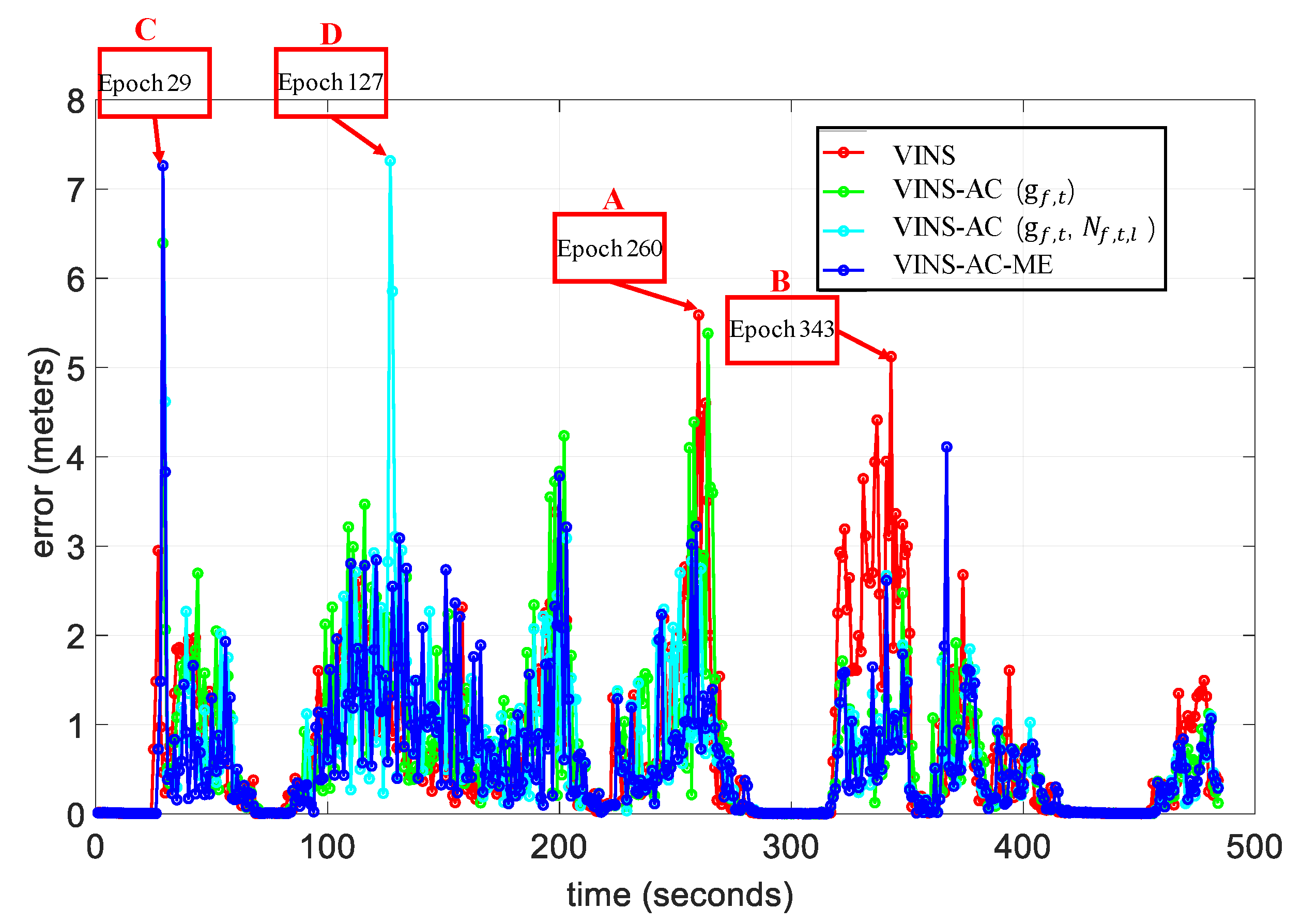
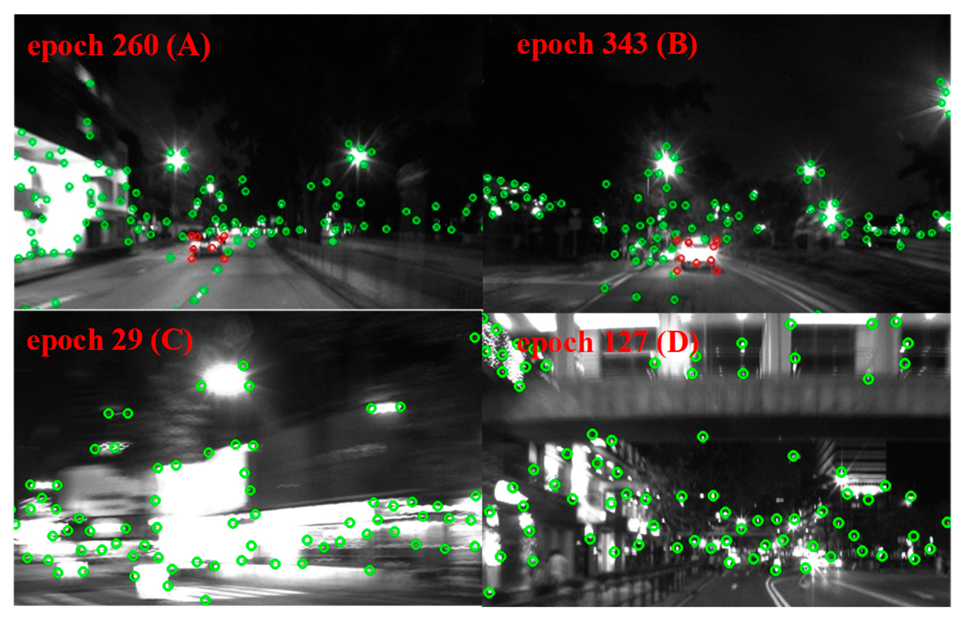
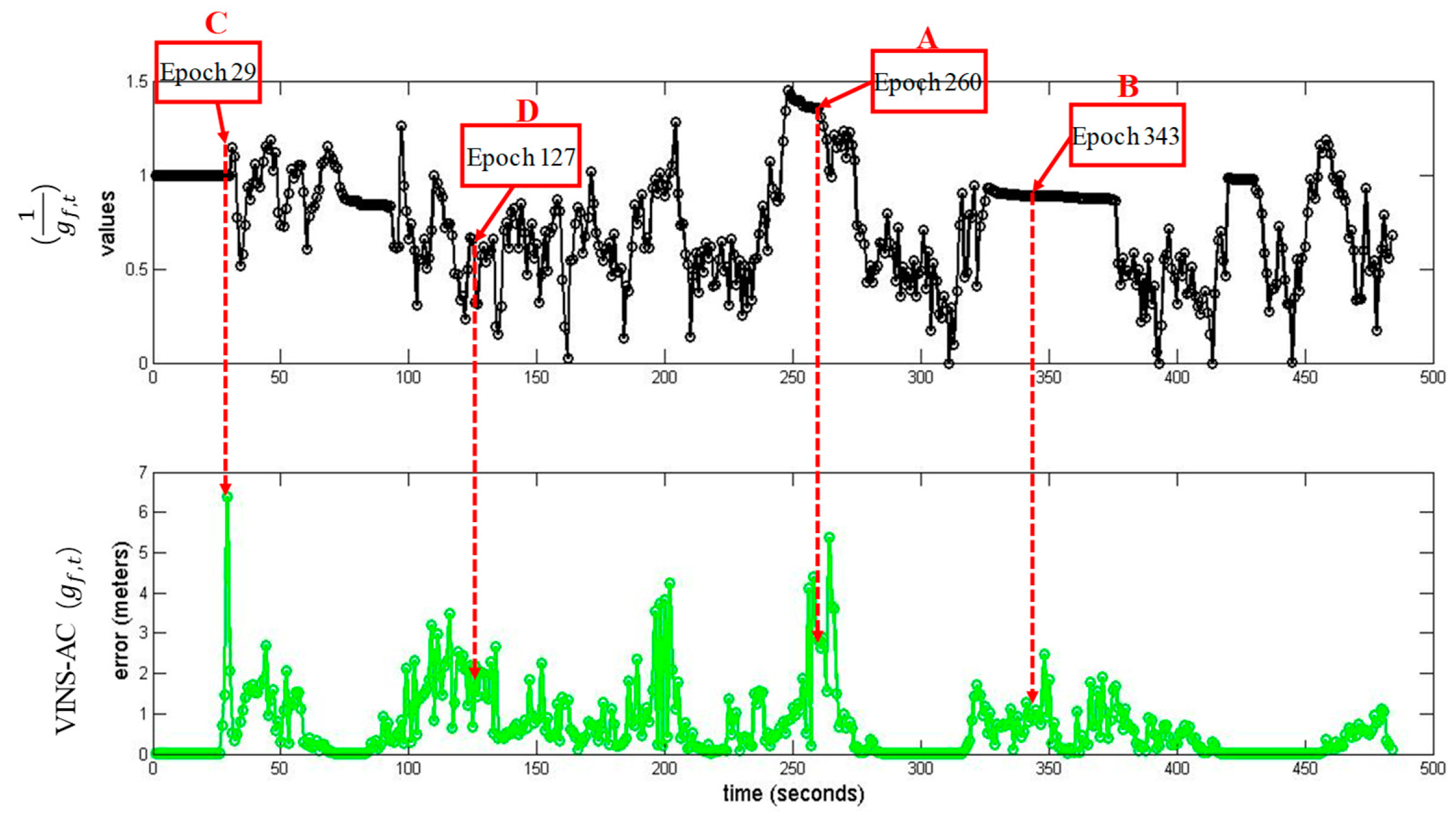
| Mean Error | VINS | VINS–AC | VINS–AC–ME | |
|---|---|---|---|---|
| Epoch 260 (A) | 5.59 m | 2.81 m | 1.62 m | 1.02 m |
| Epoch 343 (B) | 5.12 m | 0.98 m | 0.78 m | 0.72 m |
| Epoch 29 (C) | 0.47 m | 6.39 m | 7.26 m | 7.26 m |
| Epoch 127 (D) | 1.65 m | 1.43 m | 7.32 m | 1.32 m |
© 2020 by the authors. Licensee MDPI, Basel, Switzerland. This article is an open access article distributed under the terms and conditions of the Creative Commons Attribution (CC BY) license (http://creativecommons.org/licenses/by/4.0/).
Share and Cite
Bai, X.; Wen, W.; Hsu, L.-T. Robust Visual-Inertial Integrated Navigation System Aided by Online Sensor Model Adaption for Autonomous Ground Vehicles in Urban Areas. Remote Sens. 2020, 12, 1686. https://doi.org/10.3390/rs12101686
Bai X, Wen W, Hsu L-T. Robust Visual-Inertial Integrated Navigation System Aided by Online Sensor Model Adaption for Autonomous Ground Vehicles in Urban Areas. Remote Sensing. 2020; 12(10):1686. https://doi.org/10.3390/rs12101686
Chicago/Turabian StyleBai, Xiwei, Weisong Wen, and Li-Ta Hsu. 2020. "Robust Visual-Inertial Integrated Navigation System Aided by Online Sensor Model Adaption for Autonomous Ground Vehicles in Urban Areas" Remote Sensing 12, no. 10: 1686. https://doi.org/10.3390/rs12101686
APA StyleBai, X., Wen, W., & Hsu, L.-T. (2020). Robust Visual-Inertial Integrated Navigation System Aided by Online Sensor Model Adaption for Autonomous Ground Vehicles in Urban Areas. Remote Sensing, 12(10), 1686. https://doi.org/10.3390/rs12101686