The Performance Analysis of INS/GNSS/V-SLAM Integration Scheme Using Smartphone Sensors for Land Vehicle Navigation Applications in GNSS-Challenging Environments

Abstract

Modern smartphones contain embedded global navigation satellite systems (GNSSs), inertial measurement units (IMUs), cameras, and other sensors which are capable of providing user position, velocity, and attitude. However, it is difficult to utilize the actual navigation performance capabilities of smartphones due to the low-cost and disparate sensors, software technologies adopted by manufacturers, and the significant influence of environmental conditions. In this study, we proposed a scheme that integrated sensor data from smartphone IMUs, GNSS chipsets, and cameras using an extended Kalman filter (EKF) to enhance the navigation performance. The visual data from the camera was preprocessed using oriented FAST (Features from accelerated segment test) and rotated BRIEF (Binary robust independent elementary features)-simultaneous localization and mapping (ORB-SLAM), rescaled by applying GNSS measurements, and converted to velocity data before being utilized to update the integration filter. In order to verify the performance of the integrated system, field test data was collected in a downtown area of Tainan City, Taiwan. Experimental results indicated that visual data contributed significantly to improving the accuracy of the navigation performance, demonstrating improvements of 43.0% and 51.3% in position and velocity, respectively. It was verified that the proposed integrated system, which used data from smartphone sensors, was efficient in terms of increasing navigation accuracy in GNSS-challenging environments.

1. Introduction

Navigation involves the determination of the time-varying position, velocity, and attitude of a moving body. Currently, navigation technologies are expanding at a phenomenal rate, especially within the civilian sector, due to the increased availability of devices such as vehicle/personal navigators, smartphones, tablets, and other handheld devices [1]. Modern mobile phones are powerful processing devices with a host of onboard technologies of interest to navigation system designers. Due to the increased accuracy and decreased cost of microelectromechanical sensors (MEMS) [2], smartphones have been outfitted with various embedded sensors, such as global navigation satellite systems (GNSSs), cameras, gyroscopes, accelerometers, and magnetometers. These improve the smartphone’s usefulness to navigation systems.

In hostile environments, such as in narrow street canyons, tunnels, or underground parking garages, GNSS signals are prone to multipath errors or to being blocked, causing the data to be insufficient for the purposes of vehicular navigation. The accelerometers and gyroscopes within a smartphone can be used to provide a relative navigation solution. In terms of integration, an extended Kalman filter (EKF) is the most popular choice as the main estimation algorithm for data fusion. GNSS is used to correct for the systematic errors associated with the inertial sensors, which are composed of biases, scale factors, and drifts, whereas the inertial navigation system (INS) is used as a bridge for seamless navigation when the GNSS experiences an outage [3,4]. Although the integration of INS/GNSS can compensate for the main drawbacks associated with low-cost INS, the navigation errors can diverge rapidly in the absence of effective GNSS data. In recent years, the use of vision-based sensors such as cameras in navigation has strongly increased because of the numerous associated advantages. Their energy consumption is low, they can be manufactured in very small sizes, and their cost is being dramatically reduced. A key problem, which is also the relative characteristic of visual methods that directly impacts the success of these applications, is the estimation of location and distance through the use of the information gathered by these visual sensors [5]. However, the solution presented by visual sensors suffers from accumulated drift over time. Hence, there is a need to fuse visual sensors with other sensors for long-term navigation.

In the literature, the integration of data from smartphone sensors for navigation purposes has been investigated by many researchers. Walter et al. [6] proposed a system for car navigation involving the fusion of data from internal smartphone sensors (e.g., gyroscope data) with car sensor data (e.g., speed information) to support navigation using the Global Positioning System (GPS). Although the results showed that the system was able to maintain higher positioning accuracy during GPS dropouts, this system utilized only the gyroscope among the many other available smartphone sensors for the strapdown algorithm. Niu et al. [7] utilized data from the inertial sensor of an iPhone 4 to aid in GPS positioning for car navigation. The results from road test showed that the MEMS inertial measurement unit (IMU) could be used to enhance the GPS positioning. Additionally, the nonholonomic constraints (NHC) [8] could be used to improve the navigation performance significantly. However, in this research, data from another GPS receiver was used in the testing instead of the smartphone GPS data. Gikas and Perakis [9] presented a rigorous performance evaluation of smartphone GNSS/IMU sensors for intelligent transportation systems (ITS) applications. The research involved performing vehicle cruising and maneuvering tests with two kinds of smartphones. However, this study addressed only the individual performance of each sensor, and did not address an integrated solution. Al-Hamad and El-Sheimy [10] focused on using smartphones as part of a mobile mapping system (MMS). In this work, the solutions from the smartphone’s MEMS-based IMU and low-cost GPS receiver were used as the initial values for the exterior orientation parameters (EOPs) of each image. However, this work mainly focused on a mapping application instead of trajectory evaluation. Zeng et al. [11] performed a study investigating seamless pedestrian navigation using smartphone sensors. Many smartphone sensors were utilized in this work. However, some of them were used for the purpose of indoor and outdoor environmental identification. Despite the importance of vehicular navigation, this work focused only on pedestrian navigation based predominantly on the pedestrian dead reckoning (PDR) algorithm. Yan et al. [12] proposed a novel three-dimensional (3D) passive vision-aided PDR to continuously track user movements on different floors of a building by integrating the results of inertial navigation and the faster R-CNN (Regions with convolutional neural network features)-based real-time pedestrian detection. The test results demonstrated that the proposed method achieved the levels of 3D accuracy required by several emergency services. However, the visual detection used in this work was applied to floor plan detection. Wu et al. [13] presented a square-root inverse sliding window filter (SR-ISWF) for a vision-aided inertial navigation systems (VINS) and conducted experiments using a commercial-grade Samsung S4 mobile phone. Although the experimental results demonstrated the same level of estimation accuracy as state-of-the-art VINS algorithms, this study only involved testing the system within an indoor environment over a short travel distance. Speroni et al. [14] proposed a low-cost visual simultaneous location and mapping (V-SLAM) prototype using webcams and an Android smartphone for outdoor applications. The authors performed an experiment using their system in a car and provided preliminary results. However, this study involved the use of stereoscopic cameras instead of smartphone cameras. Hence, time synchronization was arguably a problem. Moreover, this work lacked a reference system to enable the generation of a reference trajectory (ground truth trajectory) for accuracy evaluation.

To the best of our knowledge, there are no studies that have rigorously investigated fusing data from IMU, GNSS chipset, and camera from smartphone for long-term land vehicle navigation applications in GNSS-challenging environments. The three main contributions of this work can be summed up as follows. First, a self-developed smartphone app was used for experimental data collection to avoid the problem of time synchronization between sensors. Second, the problem of scale in monocular solutions was solved at the beginning using measurements from GNSS chipset before this information was utilized to update the integrated filter. Finally, the proposed scheme was tested in different GNSS-challenging environments together with a high-precision reference system to verify its performance.

The remainder of the paper is organized as follows. Section 2 presents the proposed integration scheme, EKF-based data fusion, and overview of V-SLAM. Section 3 describes the field test and data processing strategy. The experimental results and discussion are then presented in Section 4. Finally, some concluding remarks and a brief outline for future research are presented in Section 5.

2. Methods

2.1. Integration Scheme

The proposed integration scheme is illustrated in Figure 1. Taking the stability of the structure and the computational cost of multi-sensor fusion into consideration, the system made use of a loosely coupled scheme of INS/GNSS/V-SLAM integration.

The IMU measurements were processed using an INS mechanization to provide a navigation solution which accounted for position, velocity, and attitude with an unbounded error in the navigation frame. The GNSS provided the absolute position as the predominant measurement update. For the camera, oriented FAST (Features from accelerated segment test) and rotated BRIEF (Binary robust independent elementary features)-simultaneous localization and mapping (ORB-SLAM) [15] were chosen as the V-SLAM method to process the data and provide measurement updates. Finally, these data were fused together using an EKF estimation algorithm.

2.2. Model Design

The core system dynamics estimation model incorporated the inertial navigation equations in a local level frame [16,17].

$$\left[\begin{array}{c}\dot{r^l}\\ \dot{v^l}\\ \dot{R_b^l}\end{array}\right]=\left[\begin{array}{c}{D}^{-1}{v}^l\\ R_b^l{f}^b-\left(2{\mathsf{\Omega }}_{ie}^l+{\mathsf{\Omega }}_{el}^l\right)v^l+g^l\\ R_b^l\left({\mathsf{\Omega }}_{ib}^b-{\mathsf{\Omega }}_{il}^b\right)\end{array}\right]$$

(1)

where $\dot{r^l}$ is the time derivative of the position in the local level frame; $\dot{v^l}$ is the time derivative of velocity; $\dot{R_b^l}$ is the time derivative of attitude; $f^b$ is a specific force, sensed by the accelerometer; ${\mathsf{\Omega }}_{ib}^b$ is the angular velocity of the body frame relative to the inertial frame, parameterized in the body frame; $R_b^l$ is the transformation matrix used to convert the body frame to the local level frame; and ${\mathsf{\Omega }}_{ie}^l$ and ${\mathsf{\Omega }}_{el}^l$ are the rotation rate of the Earth with respect to the inertial frame and the rotation rate of the local level frame with respect to the Earth, respectively. The matrix $D^{-1}$ converts the linear velocity values to angular changes in latitude and longitude:

$$D^{-1}=\left[\begin{array}{ccc}0& \frac{1}{M+h}& 0\\ \frac{1}{\left(N+h\right)cos\varphi }& 0& 0\\ 0& 0& 1\end{array}\right]$$

(2)

where $M$ and $N$ are radii of curvatures in the meridian and prime vertical of the reference ellipsoid, respectively [18]. $\varphi$ and $h$ are latitude and altitude, respectively.

In practicality, to avoid a singularity, a quaternion is used to express the attitude.

During operation, the measured acceleration and rotation rate suffer from biases, scale factors, and signal noise.

$${\widehat{f}}^b=f^b+S_f{f}^b+b_f+w_b$$

(3)

$${\widehat{\mathsf{\Omega }}}_{ib}^b={\mathsf{\Omega }}_{ib}^b+S_{\mathrm{w}}{\mathsf{\Omega }}_{ib}^b+b_w+w_w$$

(4)

To determine and compensate for those errors in IMU measurement, the bias, scale factor, and noise of the accelerometer and gyroscope have to be included in the system dynamics estimation model.

The state model can be expressed in the following form [19]:

$$\dot{x}=Fx+Gw$$

(5)

Its discrete-time equation is as follows:

$$x_{k+1}={\Phi }_k{x}_k+w_k$$

(6)

where $x={\left[\begin{array}{ccc}\delta r& \delta v& \begin{array}{ccc}\delta \mathsf{\psi }& b_g& \begin{array}{ccc}{b}_a& s_g& s_a\end{array}\end{array}\end{array}\right]}_{21\times 1}^T$ is the state vector which includes the components of position, velocity, attitude error, biases, and the scale factors of the gyroscope and accelerometer, respectively. $F$ is the state continuous time transition matrix, ${\Phi }_k$ is the state discrete-time transition matrix from epoch k to k + 1, and $w_k$ is the system noise [20,21].

For GNSS measurements, the solution available from a smartphone includes only position. The EKF measurement model can be expressed as follows:

$$z_{GNSS}=\left(r_{INS}-r_{GNSS}\right)=H_{GNSS}{x}_k+v_k$$

(7)

where $r_{INS}$ and $r_{GNSS}$ are positional vectors provided by INS and GNSS, respectively;vGPS $H_{GNSS}=\left[\begin{array}{ccc}{I}_{3\times 3}& 0_{3\times 3}& 0_{3\times 15}\end{array}\right]$ is the mapping matrix describing the relationship between the measurement and the state vector; and $v_k$ ηris the noise in the GNSS positional measurements.

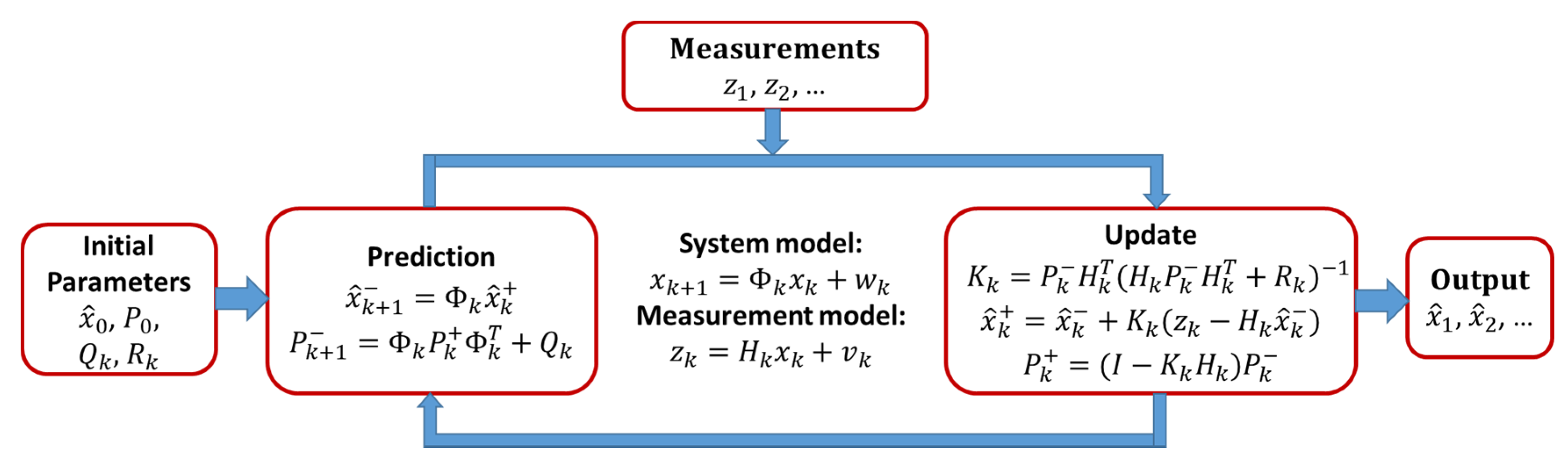
2.3. Estimation Using EKF

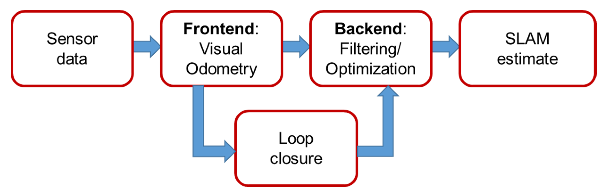
EKF equations are divided into two groups: Time predictions and measurement updates [22]. The time prediction equations are responsible for the forward time transition of the current epoch (k) state to the following epoch (k + 1) state. The time prediction equations are as follows:

$${\widehat{x}}_{k+1}^{-}={\Phi }_k{\widehat{x}}_k^{+}$$

(8)

$$P_{k+1}^{-}={\Phi }_k{P}_k^{+}{\Phi }_k^T+Q_k$$

(9)

where (ˆ) denotes estimation, ${\Phi }_k$ is the model transition matrix, $P_k$ is the estimated covariance matrix of the system state, $Q_k$ is the system noise matrix, (−) denotes the estimated values after prediction, and (+) denotes the estimated values after update.

The measurement update equations incorporate new measurements into the state estimate equations and are given as:

$$K_k=P_k^{-}{H}_k^T{\left(H_k{P}_k^{-}{H}_k^T+R_k\right)}^{-1}$$

(10)

$${\widehat{x}}_k^{+}={\widehat{x}}_k^{-}+K_k\left(z_k-H_k{\widehat{x}}_k^{-}\right)$$

(11)

$$P_k^{+}=\left(I-K_k{H}_k^T\right)P_k^{-}$$

(12)

where $K_k$ is the Kalman gain and $R_k$ is the measurement covariance matrix. All noise terms were considered to be white sequences with known covariance. The components and sequence of the computational steps are shown in Figure 2.

2.4. V-SLAM

SLAM is the process of using sensors to build a map of an unknown environment and simultaneously estimating the sensors’ pose in this environment [23]. SLAM has been an attractive research topic over the last few decades in the fields of robotics and computer vision [15,24], and has recently expanded into other application areas, such as vehicle navigation. There are many kinds of sensors that can be used in association with the SLAM technique, such as cameras, laser sensors, or sonar sensors [25,26]. Cameras are inherently cheap, low in energy consumption, and provide rich information about the surrounding environment. Therefore, many researchers focus on using cameras in SLAM applications [27,28]. Because cameras are used as the main sensor, the technique is termed V-SLAM. The flowchart describing the V-SLAM technique is shown in Figure 3.

V-SLAM methods are mainly classified into two categories based on the number of cameras used: Monocular and stereo methods [29]. Each of them has its own advantages and disadvantages in terms of cost, computational complexity, and flexibility. Stereo V-SLAM, which involves two cameras, is an expensive and complex system. Although stereo systems can retrieve image scale and depth information to provide 3D vision, they can be degraded to a monocular system when the distance to the scene is much larger than the distance between the two cameras [30]. In contrast, monocular V-SLAM utilizes only one camera. It is thus a low-cost, lightweight system, and is suitable for applications involving small robots and smartphone cameras. Despite the advantages of a monocular system, it suffers greatly from scale problems. Therefore, it is necessary to integrate monocular V-SLAM along with other systems to achieve absolute scale.

There are two different methodologies that are predominant in V-SLAM: Filtering methods and keyframe methods [30]. Filtering methods involve the camera poses and all the map features being utilized in processing at every frame. However, keyframe methods involve the camera pose being estimated using a subset of the entire map without the need to update the map features at every processed frame. Processing time is thus significantly reduced for keyframe methods, which makes them potentially applicable to real-time applications. Moreover, the filtering methods make use of the linearization process, so they suffer from accumulation errors. Overall, keyframe methods possess certain advantages over filtering methods in terms of processing time and accuracy.

ORB-SLAM, a currently available keyframe-based V-SLAM system built on excellent algorithms developed in recent years using ORB features [31] for all SLAM tasks, allows for more robust vision based navigation. ORB-SLAM is based on three main tasks: Tracking, mapping, and loop closing. Tracking is used to localize the camera with every frame and determine when to insert a new keyframe, while the mapping processes new keyframes and performs local bundle adjustment (BA) to achieve an optimal reconstruction of the surroundings of the camera pose. Finally, loop closing searches are performed with every new keyframe [32]. The complete ORB-SLAM system includes three subsystems for the purpose of processing data from monocular, stereo, and RGB-D cameras. In this present study, a monocular ORB-SLAM system was selected as the main algorithm for processing the image sequence from the smartphone cameras to provide up-to-scale translation expressed in the initial camera frame.

As mentioned above, the translation provided by the monocular V-SLAM is of an undefined scale. In order to use this translation to update the integration system, the following transformation processes were implemented. First, the translation was rescaled with the assistance of the GNSS measurement to determine metric distances. We utilized a short distance, which was initially extracted using GNSS measurements in an open sky to calculate the scale coefficient. This scale coefficient was then used to scale the monocular V-SLAM by applying the following equations:

$$\mathsf{\lambda }=\frac{\Vert t^{GNSS}\Vert }{\Vert t^{SLAM}\Vert }$$

(13)

$${}^{w}t{}_{F_i,F_{i+1}}^{SLAM}=\mathsf{\lambda }\ast {}^{c}t{}_{F_i,F_{i+1}}^{SLAM}$$

(14)

where $\Vert t^{GNSS}\Vert$ is the distance derived from the GNSS position and $\Vert t^{SLAM}\Vert$ is the corresponding translation from the V-SLAM. ${}^{c}t{}_{F_i,F_{i+1}}^{SLAM}$ and ${}^{w}t{}_{F_i,F_{i+1}}^{SLAM}$ are translations between consecutive images up-to-scale and absolute scale, respectively.

This translation vector in the camera frame was then converted into velocity in the body frame using the following equation:

$$v_{SLAM}^b=C_c^b\frac{t_{SLAM}^c}{\Delta t}$$

(15)

where $t_{SLAM}^c$ and $\Delta t$ are translation of the absolute scale and time period between consecutive images, respectively. $C_c^b$ is the rotation matrix from the camera frame to body frame, determined using a calibration process.

The velocity in the body frame was formed in the measurement model together with the NHC [8].

$$z_{SLAM}=\left(\begin{array}{c}{v}_{x-INS}^b-v_{x-SLAM}^b\\ v_{y-INS}^b-0\\ v_{z-INS}^b-0\end{array}\right)=H_{SLAM}{x}_k+v_k$$

(16)

where $v_{x-INS}^b$, $v_{y-INS}^b$, and $v_{z-INS}^b$ are velocities provided by the INS mechanization in the x, y, and z directions of the body frame, respectively. $v_{x-SLAM}^b$ is the velocity provided by the monocular V-SLAM in the x direction of the body frame and $H_{SLAM}=\left[\begin{array}{ccc}{0}_{3\times 3}& I_{3\times 3}& 0_{3\times 15}\end{array}\right]$ is the design matrix describing the relationship between the measurement and the state vector.

3. Field Test Description and Data Processing Strategy

3.1. Navigation Sensor and Field Work

3.1.1. Tested Smartphones and Reference Navigation System

Two ordinary smartphone devices were tested in this study, namely the Sony Xperia Z3 and Lenovo Tango. Although these devices are not the latest models released by their respective manufacturers, they are still very recent and used extensively worldwide. Both devices comprised a camera, GNSS chipset, and MEMS IMU that featured three-axial accelerometer and gyroscope sensors. Additionally, their processing power enabled seamless operation, minimizing the effect of errors induced by components other than the sensors being accessed. A summary of the technical characteristics of both devices is shown in

Table 1. Technical characteristics of tested smartphones.

	Sony Xperia Z3	Lenovo Tango
Processor	Qualcomm MSM8974AC	Qualcomm MSM8976
	Snapdragon 801 (28 nm);	Octa-core (4 × 1.8 GHz Cortex-A72 & 4 × 1.4 GHz Cortex-A53)
	Quad-core 2.5 GHz Krait	A-GPS, GLONASS
GNSS chipset	A-GPS, GLONASS, BDS	BMI160 (BOSCH)
Accelerometer	BMA2 × 2 (BOSCH)	BMI160 (BOSCH)
Gyroscope	BMG160 (BOSCH)	16 MP, PDAF
Camera	20.7 MP, AF	Octa-core (4 × 1.8 GHz Cortex-A72 & 4 × 1.4 GHz Cortex-A53)

.

The navigation system used to provide the reference trajectory ground truth during the two tests was an integration of GNSS and IMU. The GNSS receiver that was used in the tests was the commercial device PwrPak7D-E1 from NovAtel. The IMU that was used in the tests was the navigation-grade iNAV-RQH (iMAR). The equipment layout and technical characteristics of these reference sensors are shown in Figure 4 and

Table 2. Technical characteristics of iNAV-RQH.

	Accelerometer	Gyroscope
Bias Instability	<15 µGal	<0.002°/h
Random Walk Noise	8 µGal/$\sqrt{\mathrm{Hz}}$	0.0018°/$\sqrt{\mathrm{h}}$

, respectively.

3.1.2. Smartphone Setup and Field Experiment

Field tests were conducted using a sport utility vehicle (SUV) as the test platform. The smartphones were seated in cradles that were firmly attached to front windshield of the SUV as shown in Figure 5. Moreover, these smartphones were roughly aligned with the vehicle frame.

The tests were conducted in an urban area of Tainan City, Taiwan. The area included many tall trees, buildings, and an underground parking lot. We started with a static period in open sky and then drove for distances of approximately 3 km and 2 km, corresponding to tests one and two, respectively. The total time taken for the first test was approximately 14 min, and that taken for the second test was approximately 12 min.

3.2. Reference Trajectory Establishment and Smartphone Data Preprocessing

3.2.1. Reference Trajectory Establishment

In land vehicle navigation applications, several processing strategies are potentially useable for estimating the reference trajectory. Depending on the integration level, the loosely or tightly coupled INS/GNSS techniques can be used [9]. The loosely coupled technique, which uses post-processed kinematic GNSS data, may provide a better solution than the tightly coupled technique. However, it requires more than four satellites to be observed, a requirement that is difficult to satisfy in GNSS-challenging environments. In this present study, the tightly coupled strategy was applied together with a smoother using the commercial INS/GNSS processing software package Inertial Explore (IE) 8.90. There were lever-arms between the reference system and the smartphones, so the “true” position and velocity were transformed to the center of the smartphones when exporting the reference solutions from the IE software.

Figure 6 shows the number of visible satellites (red circles) and the position dilution of precision (PDOP) [17,33] values (blue asterisks) in the first test. It can be seen from the figure that the system sometimes had access to only a few satellites or even suffered a complete loss of satellites visible to the receiver (e.g., the time interval from 400 s to 500 s). This led to large PDOP values. As shown in Figure 7a, due to these bad conditions, the standard deviation (std) of the GNSS-only solution became larger. Figure 7b shows the std of the INS/GNSS integration solution incorporating smoothing. As mentioned in Section 3.1.1, a navigation-grade IMU was used together with a tightly coupled integration strategy to generate the reference trajectory. Therefore, the std in the north, east, and up directions remained smaller than 0.2 m during the first test.

The PDOP and number of satellites visible to the receiver in the second test are shown in Figure 8 and the std of the GNSS-only solution is shown in Figure 9a. It is clear from Figure 8 and Figure 9a that the test was run for 650 s. However, from time 550 s and on, SUV was driven into an underground parking lot. This led to only a few satellites being visible to the receiver and no solution from the GNSS-only approach. Figure 9b shows the std of the solution from the tightly coupled INS/GNSS with smoother. It can be seen from the figure that until time 550 s, the std in the three directions was smaller than 0.2 m. During the time that the SUV was in the underground parking lot, the std of the solution in three directions rose to 0.6 m.

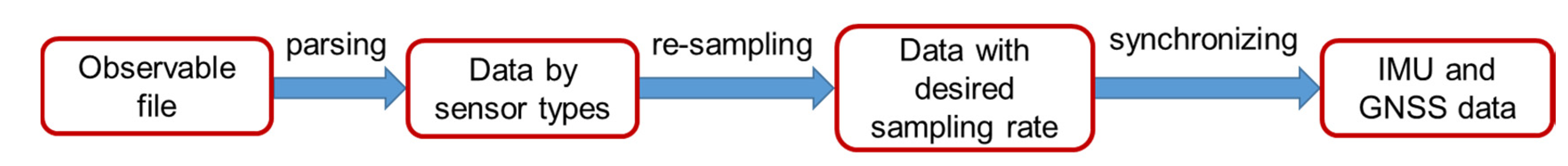
3.2.2. Smartphone Data Recording and Preprocessing

Many free smartphone apps have recently become available for sensor data collection. However, it is difficult to find an app that can simultaneously record data from the IMU, GNSS chipset, and camera. In order to overcome this problem, some of our laboratory staff members developed an Android smartphone app which enabled the simultaneous collection of data from these sensors. The raw data included a video file and a mixed file incorporating the GNSS position and IMU (accelerometer and gyroscope) observations. This observable file was parsed by sensor types. They were then resampled at the desired sampling rate. A sampling rate of 50 Hz was chosen for the purposes of this study. Finally, accelerometer and gyroscope data were synchronized together as IMU data. The flowchart of this process is shown in Figure 10.

4. Results and Discussion

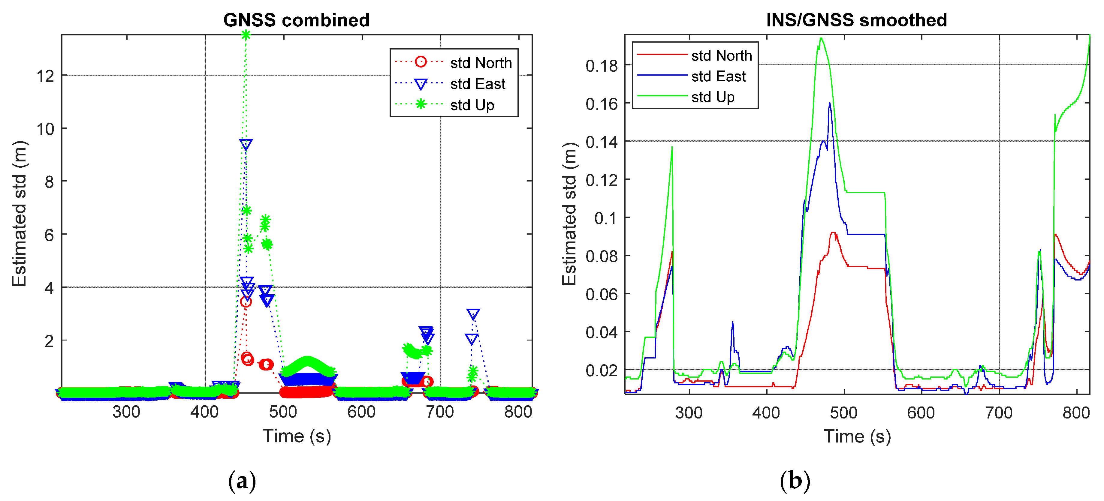
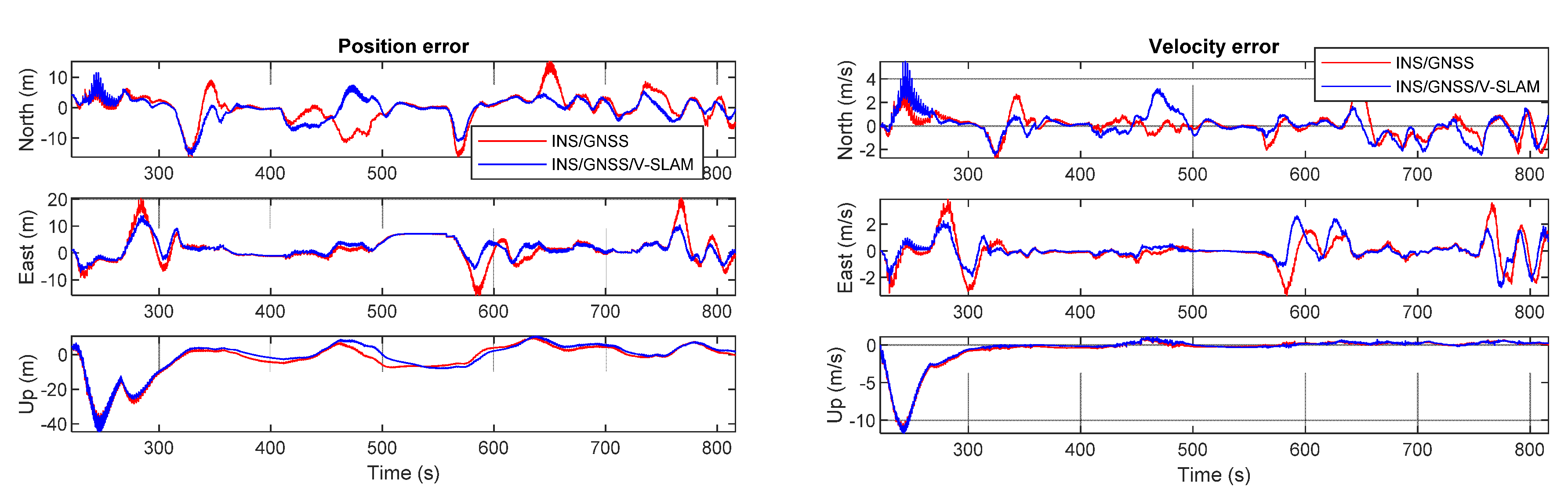
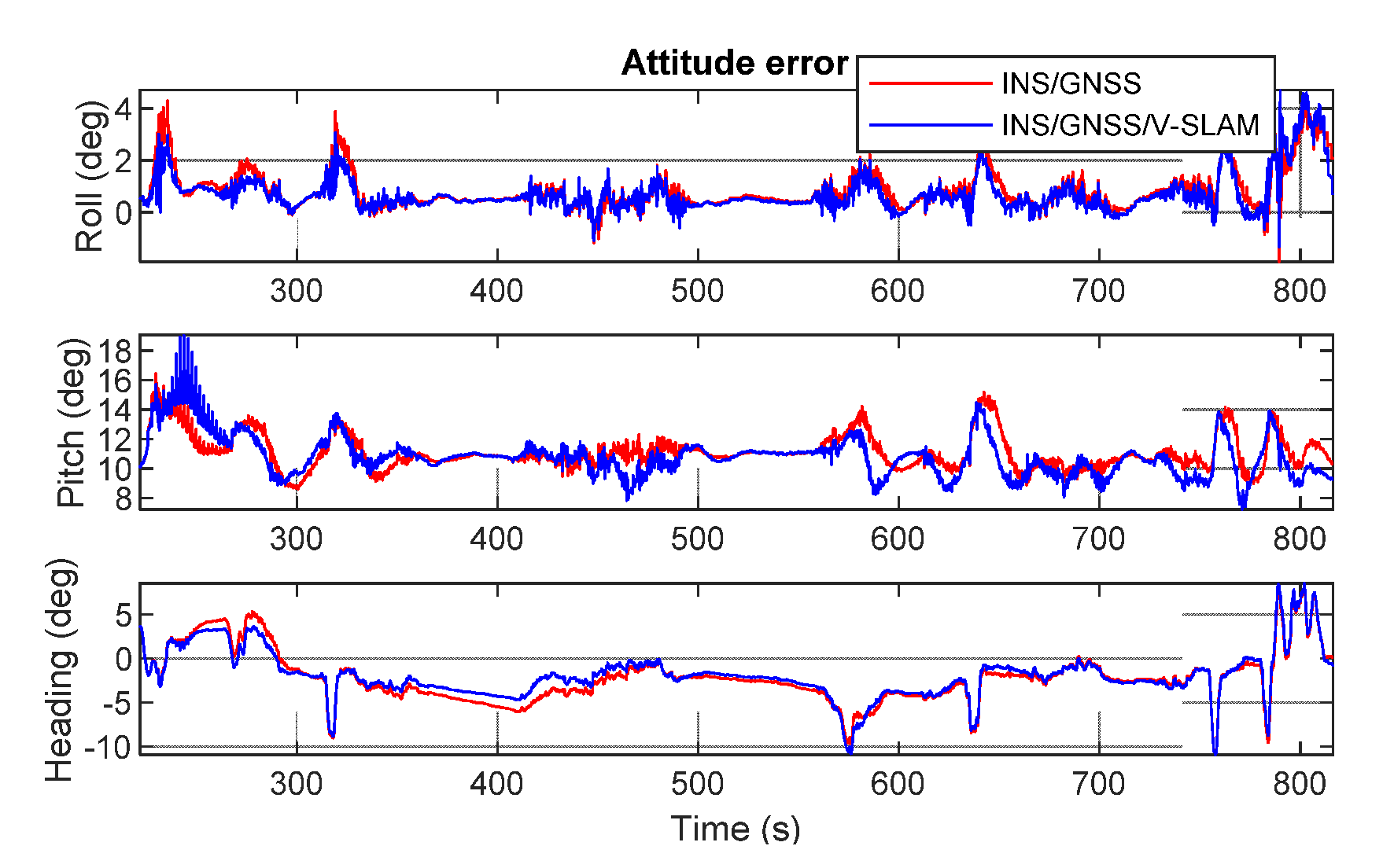
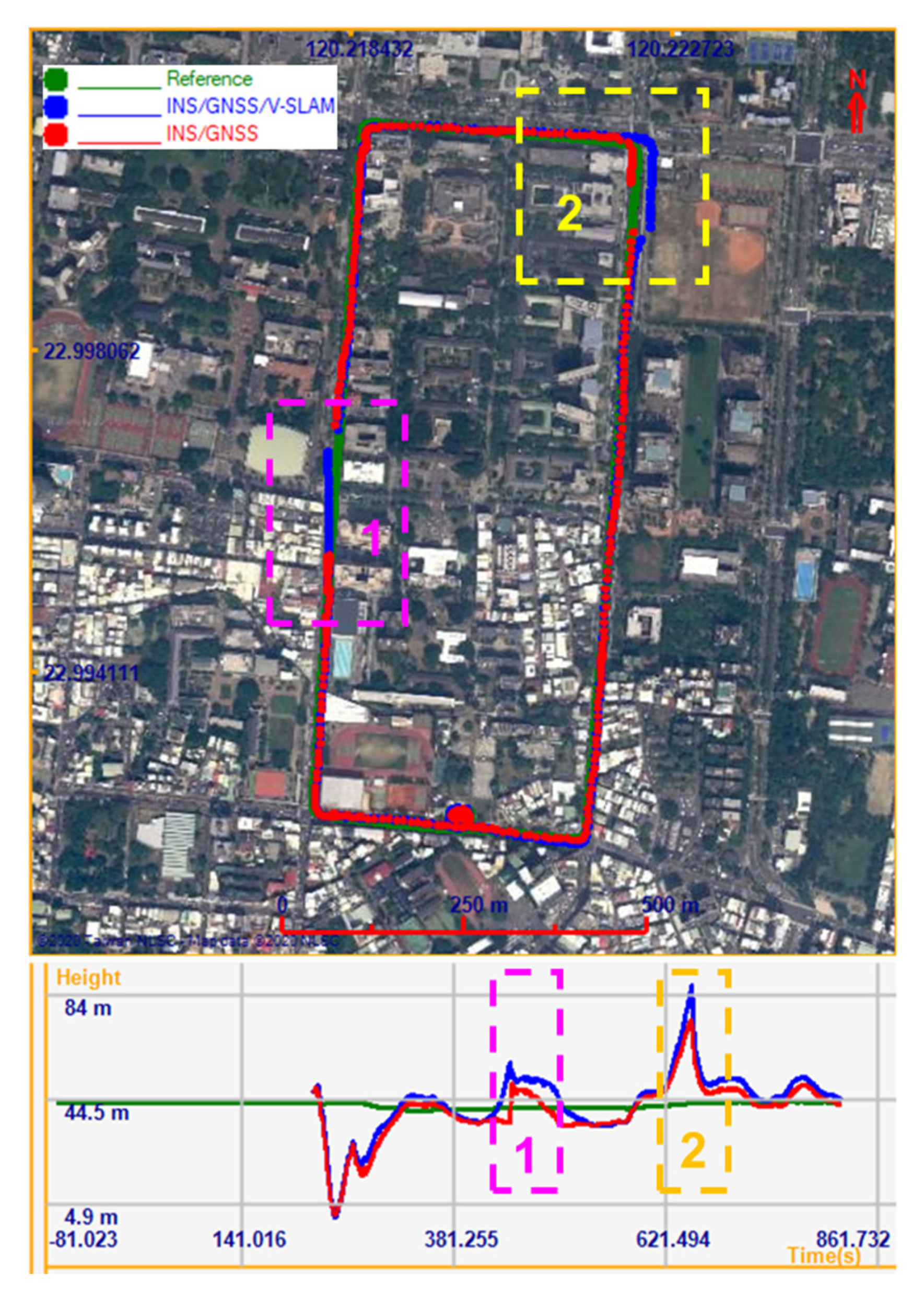
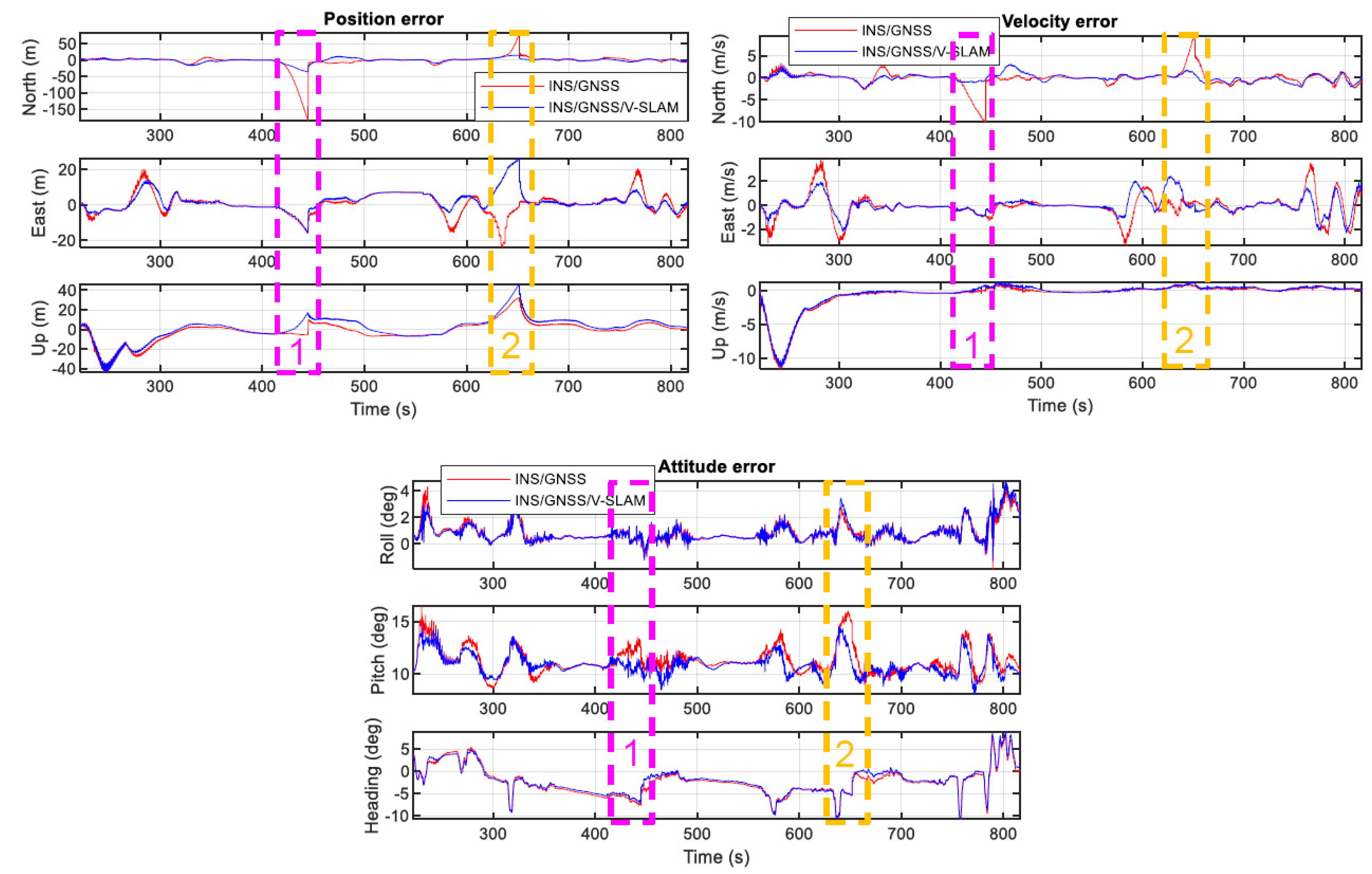
4.1. Test Results Using Sony Xperia Z3

In the first experiment, the Sony Xperia Z3 was used to test our proposed method. The testing was carried out along the streets of Tainan City, Taiwan. The test trajectory is shown in Figure 11. In the performance evaluation, the solutions provided by V-SLAM, the integration of the INS/GNSS integration aided by the NHC, and the INS/GNSS/V-SLAM integration using an original EKF were analyzed. Figure 11 shows the horizontal positions of these solutions on the map and the vertical positions on the plot below the map. It is clear from the figure that the solution from V-SLAM accumulated drift over time. In comparison to the reference trajectory (the actual trajectory), the positional root-mean-square error (RMSE) of this solution in the north, east, and up directions was 39.6 m, 31.0 m, and 5.5 m, respectively. The 3D RMSE was 50.6 m.

Figure 12 shows graphs obtained by comparing the test solutions and the reference, showing the navigation errors for position, velocity, and attitude in the first, second, and third subplots, respectively. All plots show the error in the north, east, and up directions. The numerical statistics in terms of RMSE are shown in

Table 3. Statistical summary of navigation errors in the first test.

	RMSE	INS/GNSS Integration	INS/GNSS/V-SLAM Integration
Position	North (m)	4.719	3.791
	East (m)	4.982	3.864
	Up (m)	9.471	9.488
	3D (m)	11.696	10.924
	Improvement (%)	-	6.6
Velocity	North (m/s)	0.935	1.016
	East (m/s)	0.978	0.760
	Up (m/s)	2.104	2.082
	3D (m/s)	2.501	2.438
	Improvement (%)	-	2.5
Attitude	Roll (deg)	1.138	1.022
	Pitch (deg)	11.194	10.919
	Heading (deg)	3.633	3.289
	Heading Improvement (%)	-	9.5

. As can be seen from the results, the 3D positional error of the INS/GNSS integration solution using EKF was 11.7 m, which was 76.9% higher than that of the V-SLAM solution. For the INS/GNSS/V-SLAM integration, the positional accuracy improved to 78.5% than that of the V-SLAM solution. However, in comparison to the navigation solution from INS/GNSS integration, the result from INS/GNSS/V-SLAM improved only slightly in terms of position, velocity, and heading errors with improvements of only 6.6%, 2.5%, and 9.5%, respectively.

In this experiment, the GNSS environment was not very challenging. The role of V-SLAM in improving the INS/GNSS system was thus not very clear. In order to demonstrate the efficiency of the proposed integration scheme, we planned two GNSS signal outages of 30 s in different scenarios. Figure 13 shows the trajectories of the various solutions with the planned GNSS signal outages. As highlighted in the magenta rectangle (scenario 1), during the planned 30 s GNSS signal outage on the side of the rectangular route, the INS/GNSS integration with NHC (red points) did not provide a good trajectory. V-SLAM helped to propagate the position as a bridge when no GNSS measurement update was available in the INS/GNSS/V-SLAM integration (blue points). As highlighted in the yellow rectangle (scenario 2), the planned 30 s GNSS signal outage occurred at the corner of the rectangular route. Due to aid provided by NHC, the INS/GNSS integration solution did not suffer from off-track error but suffered deeply from along-track error, while the accumulated drift remained small in the INS/GNSS/V-SLAM integration solution.

Figure 14 shows a comparison of the navigation errors of the various solutions and

Table 4. Statistical summary of navigation errors with planned GNSS outages in the first test.

	RMSE	INS/GNSS Integration	INS/GNSS/V-SLAM Integration
Position	North (m)	21.696	7.074
	East (m)	5.904	5.791
	Up (m)	10.681	11.801
	3D (m)	24.893	14.928
	Improvement (%)	-	40.0
Velocity	North (m/s)	1.813	0.862
	East (m/s)	0.976	0.740
	Up (m/s)	2.108	2.056
	3D (m/s)	2.946	2.349
	Improvement (%)	-	20.3
Attitude	Roll (deg)	1.134	1.137
	Pitch (deg)	11.323	10.927
	Heading (deg)	3.895	3.720
	Heading Improvement (%)	-	4.5

summarizes the navigation RMSE errors in both scenarios. As the graphs show, the positional accumulation errors in the north direction of the INS/GNSS solution were approximately 180 m and 70 m during the GNSS signal outages on the side and the corner of the rectangular route, respectively, whereas these accumulated errors in the INS/GNSS/V-SLAM solution were approximately 35 m and 15 m, respectively. This clearly demonstrates that the overall navigation solution from the INS/GNSS/V-SLAM integration method was much better than the solution provided by the INS/GNSS integration method. The improvement in accuracy was reflected in a reduction in position and velocity error of 40.0% and 20.3%, respectively. In terms of heading, due to the NHC, the improvement was only 4.5%.

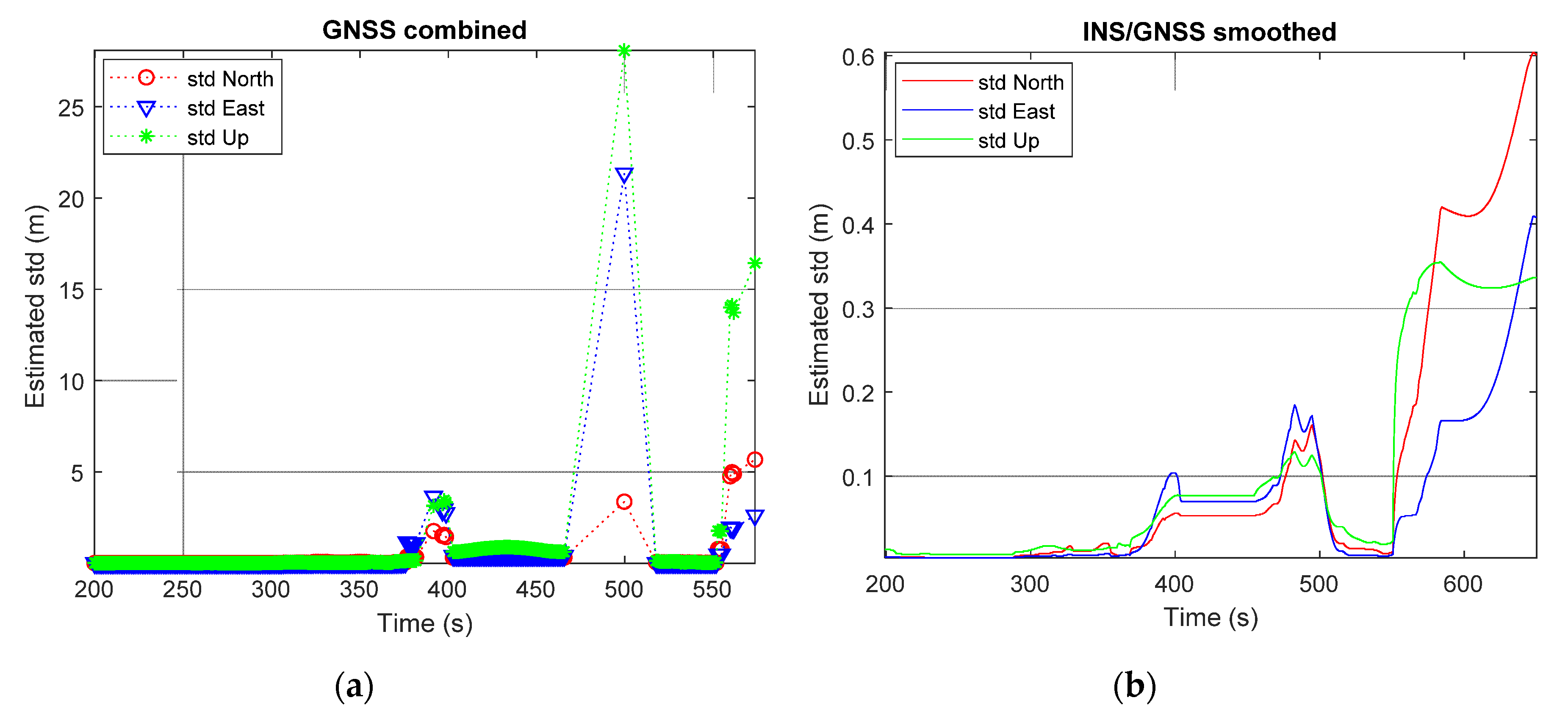
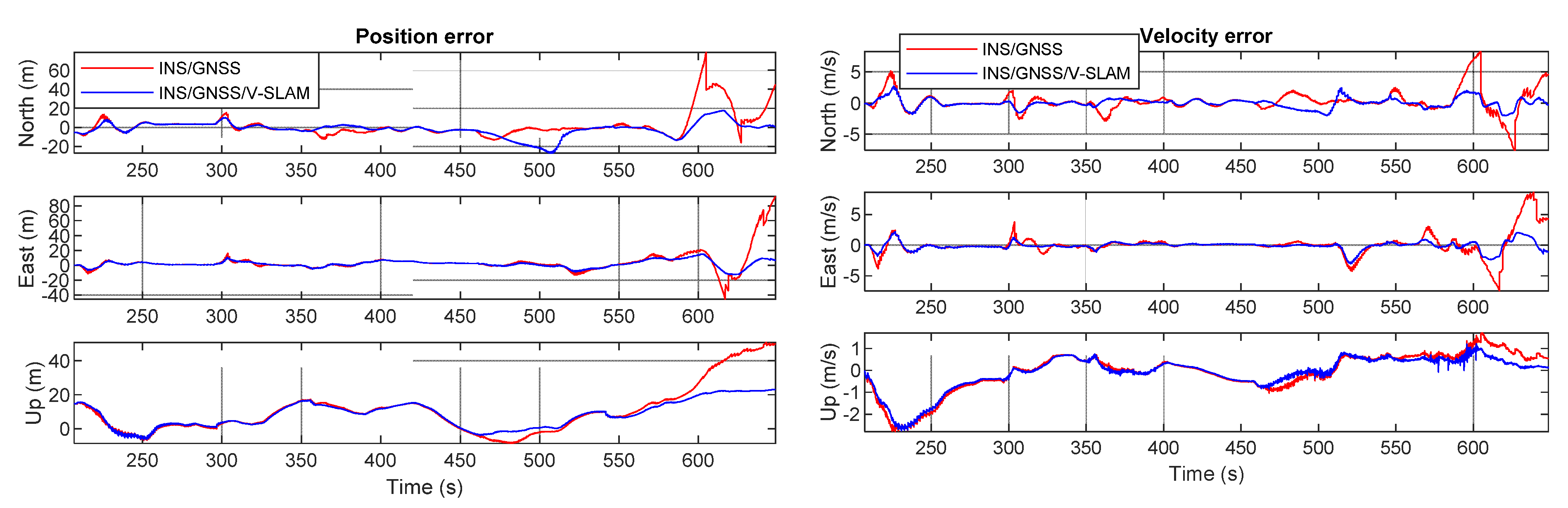
4.2. Test Results Using Lenovo Tango

In the second experiment, the Lenovo Tango was used to test our proposed method. The test field incorporated a street environment and an underground parking lot environment. The test trajectory is shown in Figure 15. In the performance evaluation, the solutions provided by V-SLAM, the INS/GNSS integration aided by the NHC, and the INS/GNSS/V-SLAM integration using EKF were analyzed. Figure 15a shows the horizontal positions of these solutions on the map and the vertical positions on a plot below the map. The magenta rectangle highlights the underground parking lot area. Figure 15b shows an enlarged detail of the trajectories in the parking lot area. It can be seen from the map that the V-SLAM trajectory, shown in cyan, accumulated over time. The trajectory of the INS/GNSS solution with NHC, shown in red, was uncontrollable when the SUV drove through the underground parking lot where the GNSS signal was blocked. The trajectory of the INS/GNSS/V-SLAM solution, shown in blue, was the best in terms of its comparison to the reference trajectory, shown in green.

Figure 16 shows graphs of the navigation errors from the various solutions in the north, east, and up directions. It is clear from the figure that during the time the GNSS signal was blocked, the INS/GNSS integration solution drifts in the north and east directions grew quickly to approximately 80 m each, whereas these drifts remained at approximately 20 m and 15 m, respectively, in the INS/GNSS/V-SLAM integration solution. The navigation RMSE error statistics are summarized in

Table 5. Statistical summary of navigation errors in the second test.

	RMSE	INS/GNSS Integration	INS/GNSS/V-SLAM Integration
Position	North (m)	12.521	7.541
	East (m)	14.234	5.022
	Up (m)	16.934	11.304
	3D (m)	25.426	14.487
	Improvement (%)	-	43.0
Velocity	North (m/s)	1.754	0.768
	East (m/s)	1.815	0.720
	Up (m/s)	0.895	0.771
	3D (m/s)	2.678	1.305
	Improvement (%)	-	51.3
Attitude	Roll (deg)	1.737	1.675
	Pitch (deg)	1.628	1.233
	Heading (deg)	6.083	5.859
	Heading Improvement (%)	-	3.7

. It can be seen from the result that the accuracy of the INS/GNSS/V-SLAM solution improved significantly in terms of position and velocity errors, with improvements of 43.0% and 51.3%, respectively, in comparison with the INS/GNSS solution. The NHC suppressed the drift error associated with the INS/GNSS solution. Hence, the heading improvement was only 3.7%.

5. Conclusions

This study proposed an integrated scheme incorporating INS, GNSS, and V-SLAM using data from smartphone sensors to overcome the weaknesses of each sensor working individually under environmental effects and the problem of unbounded error. Two ordinary smartphones incorporating a self-developed app for collecting data were used in the testing. Moreover, a system comprised of a navigation-grade IMU and a differential GNSS receiver from PwrPak7D-E1 was used to generate reference solutions.

The test results indicated that, in the GNSS-friendly environment, the solution from the INS/GNSS/V-SLAM integration using an EKF was slightly improved compared to the conventional INS/GNSS integration. However, in the GNSS-challenging environment, this improvement was significant, with up to 43.0% and 51.3% improvements in position and velocity, respectively, which verified the possibility of a robust smartphone navigation solution.

Since this work proposed the integration scheme and tested the algorithm as post-processing, for future work, this framework should be integrated into smartphone environment and run directly in this platform. In addition, nonlinear, non-Gaussian filtering will be applied to the integrated system to overcome the limitations of EKF in terms of error modelling and highly dynamic movement.

References

1. Ali, A. Low-Cost Sensors-Based Attitude Estimation for Pedestrian Navigation in GPS-Denied Environments. Ph.D. Thesis, University of Calgary, Calgary, AB, Canada, 2013. [Google Scholar]
2. Liao, J.-K.; Chiang, K.-W.; Zhou, Z.-M. The performance analysis of smartphone-based pedestrian dead reckoning and wireless locating technology for indoor navigation application. Inventions 2016, 1, 25. [Google Scholar] [CrossRef] [Green Version]
3. Titterton, D.; Weston, J. Strapdown Inertial Navigation Technology, 2nd ed.; MIT Press: Cambridge, MA, USA, 2004; Volume 207. [Google Scholar]
4. Groves, P.D. Principles of GNSS, Inertial, and Multisensor Integrated Navigation System; Artech House: London, UK, 2013. [Google Scholar]
5. Spaenlehauer, A.; Frémont, V.; Şekercioğlu, Y.A.; Fantoni, I. A loosely-coupled approach for metric scale estimation in monocular vision-inertial systems. In Proceedings of the 2017 IEEE International Conference on Multisensor Fusion and Integration for Intelligent Systems (MFI), Daegu, Korea, 16–18 November 2017; pp. 137–143. [Google Scholar]
6. Walter, O.; Schmalenstroeer, J.; Engler, A.; Haeb-Umbach, R. Smartphone-based sensor fusion for improved vehicular navigation. In Proceedings of the 2013 10th Workshop on Positioning, Navigation and Communication (WPNC), Dresden, Germany, 20–21 March 2013; pp. 1–6. [Google Scholar]
7. Niu, X.; Zhang, Q.; Li, Y.; Cheng, Y.; Shi, C. Using inertial sensors of iPhone 4 for car navigation. In Proceedings of the 2012 IEEE/ION Position, Location and Navigation Symposium, Myrtle Beach, SC, USA, 23–26 April 2012; pp. 555–561. [Google Scholar]
8. Dissanayake, G.; Sukkarieh, S.; Nebot, E.; Durrant-Whyte, H. The aiding of a low-cost strapdown inertial measurement unit using vehicle model constraints for land vehicle applications. IEEE Trans. Robot. Autom. 2001, 17, 731–747. [Google Scholar] [CrossRef] [Green Version]
9. Gikas, V.; Perakis, H. Rigorous performance evaluation of smartphone GNSS/IMU sensors for ITS applications. Sensors 2016, 16, 1240. [Google Scholar] [CrossRef] [PubMed]
10. Al-Hamad, A.; El-Sheimy, N. Smartphones based mobile mapping systems. Int. Arch. Photogramm. Remote Sens. Spat. Inf. Sci. 2014, 40, 29. [Google Scholar] [CrossRef] [Green Version]
11. Zeng, Q.; Wang, J.; Meng, Q.; Zhang, X.; Zeng, S. Seamless pedestrian navigation methodology optimized for indoor/outdoor detection. IEEE Sens. J. 2017, 18, 363–374. [Google Scholar] [CrossRef]
12. Yan, J.; He, G.; Basiri, A.; Hancock, C. 3D Passive-Vision-Aided Pedestrian Dead Reckoning for Indoor Positioning. IEEE Trans. Instrum. Meas. 2019, 69, 1370–1386. [Google Scholar] [CrossRef]
13. Wu, K.; Ahmed, A.; Georgiou, G.A.; Roumeliotis, S.I. A Square Root Inverse Filter for Efficient Vision-aided Inertial Navigation on Mobile Devices. In Proceedings of the Robotics: Science and Systems, Rome, Italy, 13–17 July 2015. [Google Scholar]
14. Speroni, E.A.; Ceolin, S.R.; dos Santos, O.M.; Legg, A.P. A low cost VSLAM prototype using webcams and a smartphone for outdoor application. In Proceedings of the 33rd Annual ACM Symposium on Applied Computing, Pau, France, 9–13 April 2018; pp. 268–275. [Google Scholar]
15. Mur-Artal, R.; Tardós, J.D. Orb-slam2: An open-source slam system for monocular, stereo, and rgb-d cameras. IEEE Trans. Robot. 2017, 33, 1255–1262. [Google Scholar] [CrossRef] [Green Version]
16. Jekeli, C. Inertial Navigation Systems with Geodetic Applications; Walter deGruyter. Inc.: Berlin, Germany, 2000. [Google Scholar]
17. Gleason, S.; Gebre-Egziabher, D. GNSS Applications and Methods; Artech House: Norwood, MA, USA, 2009. [Google Scholar]
18. Jekeli, C. Geometric Reference Systems in Geodesy (2012 edition); Ohio State University, Columbus, OH, USA. 2012. Available online: https://kb.osu.edu/bitstream/handle/1811/51274/Geometric_Reference_Systems_2012.pdf (accessed on 27 May 2020).
19. Chiang, K.-W.; Duong, T.T.; Liao, J.-K. The performance analysis of a real-time integrated INS/GPS vehicle navigation system with abnormal GPS measurement elimination. Sensors 2013, 13, 10599–10622. [Google Scholar] [CrossRef] [PubMed] [Green Version]
20. Gelb, A. Applied Optimal Estimation; MIT Press: Cambridge, MA, USA, 1974. [Google Scholar]
21. Brown, R.G.; Hwang, P.Y. Introduction to Random Signals and Applied Kalman Filtering; Wiley: New York, NY, USA, 1992; Volume 3. [Google Scholar]
22. Grewal, M.S.; Andrews, A. Kalman Filtering: Theory and Practice Using MATLAB, 2nd ed.; Wiley: New York, NY, USA, 2001. [Google Scholar]
23. Bailey, T.; Durrant-Whyte, H. Simultaneous localization and mapping (SLAM): Part II. IEEE Robot. Autom. Mag. 2006, 13, 108–117. [Google Scholar] [CrossRef] [Green Version]
24. Yousif, K.; Bab-Hadiashar, A.; Hoseinnezhad, R. An overview to visual odometry and visual SLAM: Applications to mobile robotics. Intell. Ind. Syst. 2015, 1, 289–311. [Google Scholar] [CrossRef]
25. Durrant-Whyte, H.; Bailey, T. Simultaneous localization and mapping: Part I. IEEE Robot. Autom. Mag. 2006, 13, 99–110. [Google Scholar] [CrossRef] [Green Version]
26. Cadena, C.; Carlone, L.; Carrillo, H.; Latif, Y.; Scaramuzza, D.; Neira, J.; Reid, I.; Leonard, J.J. Past, present, and future of simultaneous localization and mapping: Toward the robust-perception age. IEEE Trans. Robot. 2016, 32, 1309–1332. [Google Scholar] [CrossRef] [Green Version]
27. Aqel, M.O.; Marhaban, M.H.; Saripan, M.I.; Ismail, N.B. Review of visual odometry: Types, approaches, challenges, and applications. SpringerPlus 2016, 5, 1897. [Google Scholar] [CrossRef] [PubMed] [Green Version]
28. Afia, A.B. Development of GNSS/INS/SLAM Algorithms for Navigation in Constrained Environments. Ph.D. Thesis, University of Toulouse, Toulouse, France, 2017. [Google Scholar]
29. Lim, H.; Lim, J.; Kim, H.J. Real-time 6-DOF monocular visual SLAM in a large-scale environment. In Proceedings of the 2014 IEEE International Conference on Robotics and Automation (ICRA), Hong Kong, China, 31 May–7 June 2014; pp. 1532–1539. [Google Scholar]
30. Scaramuzza, D.; Fraundorfer, F. Visual odometry, Part 1. IEEE Robot. Autom. Mag. 2011, 18, 80–92. [Google Scholar] [CrossRef]
31. Rublee, E.; Rabaud, V.; Konolige, K.; Bradski, G. ORB: An efficient alternative to SIFT or SURF. In Proceedings of the 2011 International Conference on Computer Vision, Barcelona, Spain, 6–13 November 2011; pp. 2564–2571. [Google Scholar]
32. Mur-Artal, R.; Montiel, J.M.M.; Tardos, J.D. ORB-SLAM: A versatile and accurate monocular SLAM system. IEEE Trans. Robot. 2015, 31, 1147–1163. [Google Scholar] [CrossRef] [Green Version]
33. Kaplan, E.; Hegarty, C. Understanding GPS: Principles and Applications; Artech House: London, UK, 2005. [Google Scholar]
Figure 1. Inertial navigation system (INS)/global navigation satellite system (GNSS)/visual simultaneous location and mapping (V-SLAM) integration scheme.
Remotesensing 12 01732 g001
Figure 2. Kalman filter loop.
Remotesensing 12 01732 g002
Figure 3. V-SLAM framework.
Remotesensing 12 01732 g003
Figure 4. Reference sensor equipment layout.
Remotesensing 12 01732 g004
Figure 5. Smartphone setup in field tests: (a) Sony Xperia Z3; (b) Lenovo Tango.
Remotesensing 12 01732 g005
Figure 6. Number of visible satellites and position dilution of precision (PDOP) values in the first test.
Remotesensing 12 01732 g006
Figure 7. Estimated std from the first test: (a) GNSS-only solution; (b) INS/GNSS integration with smoothing solution.
Remotesensing 12 01732 g007
Figure 8. Number of visible satellites and PDOP values in the second test.
Remotesensing 12 01732 g008
Figure 9. Estimated std from the second test: (a) GNSS-only solution; (b) INS/GNSS integration with smoothing solution.
Remotesensing 12 01732 g009
Figure 10. Smartphone data preprocessing steps.
Remotesensing 12 01732 g010
Figure 11. Trajectories of the various solutions in the first test.
Remotesensing 12 01732 g011
Figure 12. Graphical comparison of the navigation errors associated with the various solutions in the first test.
Remotesensing 12 01732 g012aRemotesensing 12 01732 g012b
Figure 13. Trajectories of the various solutions with planned GNSS signal outage in the first test.
Remotesensing 12 01732 g013
Figure 14. Graphical comparison of navigation errors with planned GNSS outages in the first test.
Remotesensing 12 01732 g014
Figure 15. Trajectories of the various solutions in the second test (a); Carpark detail (b).
Remotesensing 12 01732 g015
Figure 16. Graphical comparison of the navigation errors associated with the various solutions in the second test.
Remotesensing 12 01732 g016aRemotesensing 12 01732 g016b