Article

Investigating the Effects of Land Use and Land Cover on the Relationship between Moisture and Reflectance Using Landsat Time Series

by
Heather J. Tollerud
*,
Jesslyn F. Brown
and
Thomas R. Loveland
U.S. Geological Survey EROS Center, Sioux Falls, SD 57198, USA
*
Author to whom correspondence should be addressed.
Remote Sens. 2020, 12(12), 1919; https://doi.org/10.3390/rs12121919
Submission received: 30 April 2020 / Revised: 2 June 2020 / Accepted: 4 June 2020 / Published: 13 June 2020

Abstract

:
To better understand the Earth system, it is important to investigate the interactions between precipitation, land use/land cover (LULC), and the land surface, especially vegetation. An improved understanding of these land-atmosphere interactions can aid understanding of the climate system and modeling of time series satellite data. Here, we investigate the effect of precipitation and LULC on the reflectance of the land surface in the northern U.S. Great Plains. We utilize time series satellite data from the 45 year Landsat archive. The length of the Landsat record allows for analysis of multiple periods of drought and wet conditions (reflecting climate, as well as weather), such that the precipitation-reflectance relationship can be investigated robustly for every individual pixel in the study area. The high spatial resolution of Landsat (30 m) allows for investigation of spatial patterns in weather (i.e., precipitation extremes) interactions with land surface reflectance at the scale of individual fields. Weather history is represented by a drought index that describes effective moisture availability, the Standardized Precipitation and Evaporation Index (SPEI). We find that effective moisture has a robust and consistent effect on reflectance over many types of land cover, with ∼90% of all pixels having significantly ( p < 0.01 ) higher visible reflectance during dry periods than during wet, occurring in nearly all regional, temporal, and LULC categories investigated. In grassland, the relationship is especially strong; there is an average reflectance increase of more than a third between very wet and very dry conditions (red band), and ∼99% of pixels have a significant relationship. In cropland, the effective moisture-reflectance relationship is more variable, suggesting that management decisions are an important factor in cropland-reflectance relationships.

Graphical Abstract

1. Introduction

The relationship between land use/land cover (LULC) and climate or weather is of profound importance in the Earth system. Changes in climate and LULC have the potential to produce substantial disruption for individuals and societies [1,2]. Interactions between LULC and weather are of particular importance for understanding the climate system, as they can amplify the impacts of changes in either, through feedbacks. Understanding these land-atmosphere interactions is critical to predicting the effects of changes in either LULC or climate on both, and on society [3].
An important instance of land-atmosphere interactions is the relationship between precipitation and surface reflectance (at a variety of wavelengths). Precipitation and the albedo of the land surface have the potential to produce feedbacks; for example, during drought, albedo usually increases, altering atmospheric energy transfer and often further inhibiting precipitation [4,5]. To improve understanding of these feedbacks, it is important to have evidence for the magnitude of both the effects of albedo on precipitation and the effects of precipitation on albedo. Estimates of the magnitude of the effect of moisture on surface reflectance at a variety of wavelengths help to improve estimates of precipitation-albedo effects and have the potential to inform modeling studies of topics such as land-atmosphere interactions and analysis of time series remote sensing data.
A number of studies have observed a change in remote sensing observations during drought or low soil moisture, e.g., [5,6,7,8,9,10], and this relationship has been investigated at length to produce drought indices [11,12]. However, these studies have generally covered short time periods (less than the 30 years commonly used in creating climate baselines), implicitly relying on a space-for-time-type approach rather than investigating every pixel location across multiple drought episodes. This approach potentially over-emphasizes the attributes of particular drought events and reduces the potential for investigating relationships across space (including between LULC classes) since pixels do not each have a robust estimate independent of other pixels. Furthermore, studies have generally investigated coarser spatial scales than 30 m Landsat data. In addition, much previous work has been focused on vegetation health rather than reflectance. Changes in vegetation are a critical part of reflectance variation, but soil moisture also affects the reflectance of the soil directly [13], so a study of the effect of weather including dry and wet extremes on a direct measurement of reflectance is valuable.
Since different land cover types (e.g., grassland, barren land, forest, and cropland) are all likely to behave differently during periods of high or low moisture, it is also critical to take LULC into consideration when investigating land-atmosphere interactions [3,14]. Grasslands tend to respond to drought quickly, with reduced evapotranspiration and leaf senescence, while evapotranspiration and gross primary productivity in some forest types can change more slowly after the initiation of drought [15,16]. The drought response of croplands can be highly variable since there is a wide variety of management regimes and irrigation practices [17]. Given the differences in LULC types, changes in LULC have the potential to affect reflectance, albedo, and climate. Land cover has a direct effect on reflectance, while land use may affect land cover. Despite the importance of LULC, there has been little work investigating the LULC dependence on large-scale drought responses.
Remote sensing time series investigations over long (multi-decadal) timescales and large (thousands of km 2 ) areas can help to distinguish underlying land-atmosphere relationships as data are gathered synoptically under a wide range of conditions. Landsat is well suited for this type of analysis, as it has extensive coverage across a long period of record (1972-current) including multiple drought episodes [18,19]. Analysis of multiple drought episodes establishes the range of observed responses to drought, allowing a focus on the average drought response of a location instead of the particularities of a specific drought. The 30 m resolution of Landsat is an advantage over studies using 250–1000 m resolution or coarser, because it enables distinguishing smaller features, including field/management boundaries. Furthermore, there are more unmixed pixels that contain only one LULC type [20]. Early data from Multispectral Scanner System instruments (MSS; first launched 1972) are lower quality and resolution (60 m) than data from more recent missions, but are still useful in this kind of study, where a long baseline is potentially more important than high radiometric accuracy [21].
Drought data are necessary to investigate effective moisture-reflectance relationships. The Standardized Precipitation-Evapotranspiration Index (SPEI) is a relatively new drought index and has been utilized by a number of studies, e.g., [22]. The SPEI indicates the water deficit compared to normal conditions for a location [23,24]. One advantage of the SPEI calculation is that it includes the effect of temperature on water availability by subtracting potential evapotranspiration (PET) from precipitation [25]. Furthermore, as the SPEI uses the same statistical approach for all environments and can be applied globally without local correction factors, it provides for the assessment of moisture conditions at any desired timescale and, thus, can describe the water stress on vegetation. Here, we understand the SPEI as a measure of effective moisture.
The goal of this paper is to evaluate the effect of LULC on the relationship between effective moisture and reflectance and to investigate methods for examining geographic patterns in this relationship across the landscape. For each 30 m pixel in the study area, we create a time series of Landsat reflectance (visible, near-IR, and shortwave-IR bands) and compare to a corresponding time series of SPEI data. Summary statistics and linear regression fits of SPEI versus reflectance are averaged by the LULC category to investigate differences among the LULC categories. Individual droughts (and individual wet periods) each have their own unique and interesting features, and so, it is important to sample as many drought events as possible to avoid interpreting patterns seen in one or two droughts as a more general result. To maximize the temporal period in this study, we include MSS data (begin in 1972) in the analysis. The results of this work are intended to contribute to models that might benefit from an improved understanding of the relationship between effective moisture and reflectance, such as time series modeling and land-atmosphere interaction modeling.

2. Study Area

This study focuses on a study area in the northern U.S. Great Plains (Figure 1). The Great Plains are a suitable location for this study because the area has experienced frequent droughts and the vegetation (which is mainly herbaceous) is responsive to precipitation [26,27]. Furthermore, research on semi-arid grasslands (including the Great Plains) is of global importance as grasslands compose >30% of the Earth’s land surface and are especially vulnerable to anthropogenic LULC conversion [28].
The study area has a semi-arid climate, with average annual precipitation ranging from ∼500 mm/y in the southeast to <400 mm/y in the northwest [29]. Precipitation is highest in the spring, with as much as half of annual precipitation falling in the May–July period. Average annual temperatures are ∼6–9 C, with average January minimums of −15 to −11 C and average July maximums of 28–32 C (based on meteorological stations within the study area, 1981–2010; Figure 2 [29]). On average, there is snow depth of an inch or more on 70 days per year [29]. Vegetation in the study area can be limited by either water or energy, depending on weather conditions.
As measured by the SPEI, large parts of the study area were in drought in 1975, 1980, 1988, 2002, 2006, and 2012. The droughts of 1980, 1988, and 2012 are noteworthy as being part of the three most expensive droughts that have occurred in the U.S. since 1980 [30]. The 2002 and 2006 droughts were less widespread, but within the study area, their intensity was second only to 1980. Wetter periods occurred in 1978, 1982, 1986, 1995, 1999, 2010–2011, and 2014. Since both wet and dry events were distributed throughout the study period, the Landsat record provided a baseline for investigating relationships that were linked to precipitation rather than to a particular drought event.
The study area is dominated by grassland (∼72%), with cropland (∼17%) and pasture/hay (∼6%) the next most common (National Land Cover Database 2001; [31]). Livestock grazing is common on grassland throughout the study area; the U.S. Department of Agriculture 2012 Census of Agriculture found 585,704 cattle and calves in the eight counties dominating the study area (4,237,738 ha total county area; [32]). Grassland in the study area is mixed-grass prairie, with species including western wheatgrass (Pascopyrum smithii), blue grama (Bouteloua gracilis), needle and thread (Stipa comata), and green needle-grass (Stipa viridula) [33]. C 3 species are most common, but C 4 grasses compose as much as 50% of production in some parts of the study area [34].
Cropland in the study area is often divided into fields that are at least 65 ha (a quarter section), but can be substantially larger. Hay and wheat are the most common crops grown in the study area. Specifically, the crops covering the most area in 2014 were non-alfalfa hay (∼31% of crop area), spring wheat (26%), winter wheat (12%), corn (9%), sunflower (5%), fallow (5%), and alfalfa (4%) (data from the Cropland Data Layer, [35]). In South Dakota, spring wheat is usually planted April 8–May 12 and harvested July 27–August 20 (this schedule takes advantage of early summer rains), winter wheat is planted September 9–October 5 and harvested July 14–August 5, and non-alfalfa hay is harvested (more than once) June 20–August 14 [36]. These dates are dependent on precipitation. Most cropland is rainfed (>99% in 2007; [37]), although early in the study period, there were small areas of irrigation distributed across the region [38]. Croplands are typically located on table lands parallel to streams.
LULC change has been moderate in the region during the past ∼40 years, with LULC change in 7.4 ± 2.0 % of the Northwestern Great Plains ecoregion in 1973–2000 [39]. Conversions between agriculture and grassland were the most frequent changes, driven by economic forces, technology, and farm policies including the Conservation Reserve Program (CRP). The CRP removed more than 200,000 ha from production between 1985 and 1992 in counties roughly encompassing the study area [40].

3. Methods

For this study, Landsat data were compared to SPEI and LULC. A Landsat reflectance time series was constructed for each 30 m pixel in the study area for visible, near-IR, and shortwave-IR bands. Each Landsat time series was then compared to a corresponding SPEI time series. Histograms of reflectance by SPEI and LULC were computed to display the general relationship between effective moisture and reflectance, and linear regression of SPEI versus reflectance was used to investigate this relationship in more detail. We included MSS to extend the temporal range to 1972, in order to incorporate as many dry and wet periods as possible in the analysis. Inclusion of MSS led us to utilize top of atmosphere (TOA) reflectance instead of surface reflectance, because atmospherically correcting MSS was more difficult than later instruments due to the lack of shortwave-IR bands [41]. We also investigated the relationship between the Landsat atmospheric correction and the drought index to evaluate the impact of the utilization of TOA in this analysis.

3.1. Landsat Data Processing

Scene-based pre-collection Landsat data from 1972–2014 were acquired from the USGS Landsat archive [20,42]. In general, all available observations from the four-scene study region shown in Figure 1 with <50% cloud cover were utilized (1430 observations, listed in Supplementary Materials S1). This included observations from MSS, Thematic Mapper (TM), Enhanced Thematic Mapper Plus (ETM+), and Operational Land Imager (OLI) instruments (Table 1). For Landsat 1–3, this area approximately covered six scenes in the Worldwide Reference System-1. Since vegetation is dormant and the ground is frequently snow covered during the winter in the study area, only dates between April 15–October 15 were included in the analysis.
One priority of this study was the utilization of data back through the MSS period of the Landsat program, in order to include 1970s era droughts in the analysis (Figure 3). Data from MSS are the earliest of this type of Earth observation, and the data archive for MSS is extensive in the study area [43]. This time period allowed the incorporation of three noteworthy droughts (1975, 1977, and 1980) in addition to four noteworthy droughts in the later record (1988, 2002, 2006, and 2012). Compared to TM, ETM+, and OLI, the MSS data have lower spatial resolution ( 60 m versus 30 m ), fewer spectral bands (4 versus ≥7), a lower frequency of observation (18 day vs. 16 day repeat cycle; <20 observations/y versus ∼60/y in the 2000s for this dataset), reduced radiometric resolution (6 bit versus 8 bit and 12 bit quantization), higher calibration uncertainty (8–11% for MSS versus 7–9% for TM and 5% for ETM+/OLI), and more data artifact issues [21]. The issues and the lack of ancillary data make the calculation of surface reflectance for MSS more difficult. Here, we utilized TOA reflectance for all instruments.
To evaluate the impact of the use of TOA reflectance instead of surface reflectance, we downloaded Landsat Collection 1 TOA and surface reflectance products (available for TM, ETM+, and OLI) for a random selection of 40 TM, 30 ETM+, and 20 OLI observations out of the 1430 Landsat observations utilized in the full dataset. Landsat surface reflectance was generated using the Landsat Ecosystem Disturbance Adaptive Processing System (TM and ETM+; [44]) and Landsat Surface Reflectance Code (OLI; [45]). After applying the cloud masks described below, we calculated the average difference between TOA and surface reflectance across the Landsat observation for each band. We then compared the mean difference for each Landsat observation to the drought index value for the scene center of that observation, to investigate the impact of the atmospheric correction on the relationship between weather and reflectance. In addition, we investigated atmospheric correction of all red band observations in the study using the dark object subtraction method [46]. This method can be applied to MSS in a straightforward way, but was potentially affected by a lack of dark objects in the study area (Appendix B).
To filter out clouds and data artifacts (particularly noticeable in MSS data), we created cloud masks for every observation semi-manually [47]. A simple cloud masking algorithm based on the Fmask algorithm [48] and optimized for the study area was used as a starting point, with Fmask overlaid for reference. More details are described in Appendix A (see also [49]). Any obvious issues with the potential impact on the analysis (including instrument artifacts, visible aerosols, cloud shadow, and snow) seen during cloud masking were masked along with the clouds. Landsat 5 observations were observed to have bright artifacts along the swath edges after activation of bumper-mode in 2002 [50]. These artifacts were located north of gaps in coverage due to scan line offsets, so to remove them automatically, we expanded the initial no-data mask 5 pixels further north along the edges of the image. All valid pixels that were not masked were utilized in our analysis. The pixel-by-pixel approach taken here minimized the influence of missing data of any kind, including Landsat 7 ETM+ scan line corrector artifacts [51].
We combined the scene-based Landsat data to produce time series data stacks. Data stacks were produced as half-degree tiles, to keep the data volume manageable within each tile and to match the spatial coverage of the drought index data. Landsat data were downloaded in Universal Transverse Mercator (UTM) and stacks produced in UTM; as the study area crosses the boundary between UTM Zones 13 and 14 (at 102°W), Landsat scenes that crossed the zone boundary were reprojected to the other UTM zone when producing tiles on the other side of the boundary from the scene center. In order for MSS data to be added to the data stack, the 60 m MSS pixels were subdivided into four identical 30 m pixels and transformed to match the rest of the data stack by nearest neighbor resampling. Images were manually inspected for multi-pixel geolocation offsets by visual comparison with other images from the same area, and problematic scenes were removed from the dataset. However, some one or two pixel geolocation errors remained, especially in MSS data and in areas of scene overlap, meaning that there was likely to be some degree of contamination between neighboring pixels that must be taken into consideration during analysis.

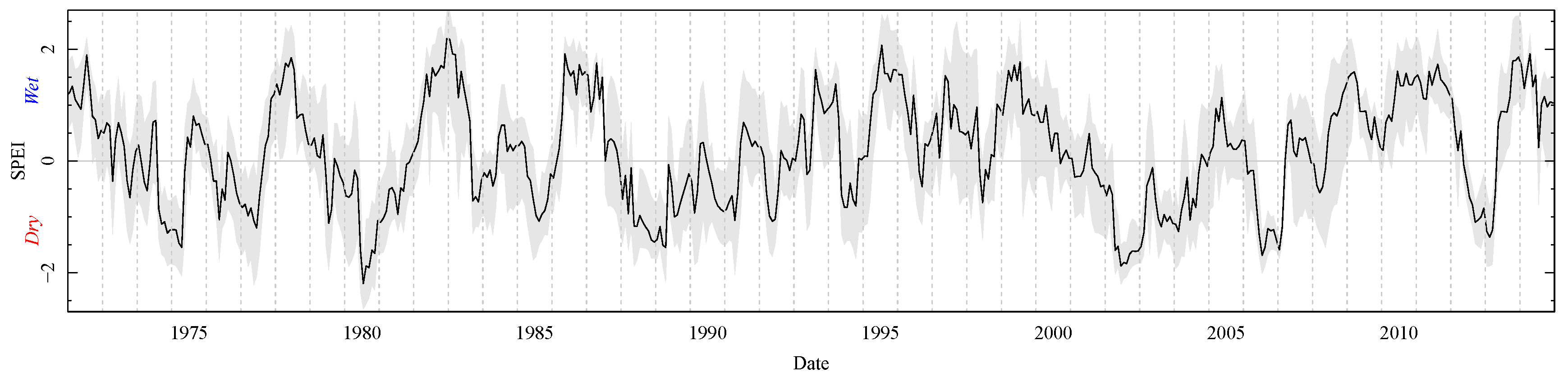
3.2. Drought Index: SPEI

We selected the Standardized Precipitation-Evapotranspiration Index (SPEI; [23]) to quantify drought in this study. The SPEI is a drought index that is calculated from PET, as well as precipitation; as we used it to investigate wet conditions in addition to dry conditions, we describe what SPEI was measuring as effective moisture. The SPEI is broadly applicable (it uses the same statistical approach in all locations), estimates drought condition based on water balance and PET, and provides for the assessment of drought conditions at any desired timescale. We utilized data from SPEIbase (Version 2.4; [52]). This dataset contains global drought data with half-degree spatial resolution and monthly temporal resolution, in the period 1901–2014 (based on Climatic Research Unit time series Version 3.23 meteorological data; [53]). This dataset is based solely on meteorological station data, so we were able to perform a comparison of two independent measurements (satellite and drought), but the spatial resolution was coarse. Negative SPEI values indicate dry (<50th percentile) conditions; −1 is one standard deviation below the average of the full time series. SPEI values during the study period covered a wide range of drought conditions (Figure 4).
One strength of the SPEI is that it can be computed over any desired timescale. The SPEI is calculated by comparing the difference between precipitation and PET over a given period of time to what would be expected based on the entire record. For example, the 9 month SPEI for October 1, 2000, would be calculated based on precipitation-PET for the period 1 January 2000 to 30 September 2000, as compared to the distribution of January-September precipitation-PET for all years 1901–2014. To simplify the current study, we focused on 9 month SPEI (i.e., based on a 9 month time period). For the summer months in this study, the 9 month timescale included the current growing season and the previous winter snow season. A shorter timescale would begin to exclude precipitation data from the previous winter and the critical spring precipitation maximum, while a longer timescale would include data from the previous growing season. Furthermore, this timescale is similar to the timescale of the Palmer Drought Severity Index [23]. Preliminary testing demonstrated that other timescales, both shorter and longer, also showed a reflectance response.
Since the SPEI dataset (available monthly, at half-degree spatial resolution) does not have the same characteristics as the Landsat observations, it was necessary to determine how to compare them. Spatially, we utilized the SPEI data for a particular half-degree area for all Landsat pixels contained within that half-degree. This meant that the 20 SPEI pixels present in the study area were each applied to ∼2 million pixels of stacked Landsat data. Temporally, the SPEI is available at monthly intervals, while Landsat observations occur throughout the month. Here, for each Landsat observation that intersected the current SPEI pixel, we linearly interpolated between the drought index at the end of the preceding month and the index at the end of the current month based on the day of the month of the Landsat observation. This method did not account for when in the month precipitation occurred, but potential issues were minimized since in the 9 month SPEI, 8 of the 9 months of input for the SPEI calculation were the same for 2 consecutive months.

3.3. Land Use/Land Cover: NLCD

Land use and land cover data at Landsat spatial resolution (30 m) are available from the National Land Cover Database (NLCD; [54]), which generally has over 80% agreement with reference data [55]. We acquired all available years of NLCD data (1992, 2001, 2006, and 2011 [31,56,57,58]). In order to focus on areas that had stable LULC throughout the study period, we selected only pixels that were in the same LULC category in all NLCD datasets (the 1992 NLCD had somewhat different categories; see Table 2). This was intended as a conservative approach to removing pixels with possible land cover change rather than as a measurement of the amount of change occurring in the study area, since the 1992 NLCD was not directly comparable to later data, and the pixels that were not used (∼30% of the total) should not be interpreted as a measure of change in the study area. A limitation of this approach is that pixels that had LULC change before 1992 would be included in the stable category. Major farm policy changes during this period were of potential importance, and some degree of LULC miscategorization in this period was plausible.

3.4. Data Analysis Methods

For each NLCD class in Table 2, we computed histograms of reflectance as a function of SPEI (reflectance bin size 0.001, selected as a number that was well below the expected error in Landsat measurements; SPEI bin size 0.5, selected to produce a reasonable number of categories for viewing). Histograms were computed for the six Landsat bands, including MSS in green and red. Since reflectance varies based on the time of the year, changes through time were investigated by including Landsat observations based on a 40 day moving window. Inclusion was based on day of year rather than calendar date. The 40 day interval was selected because it was the smallest multiple of 10 that included two full 16 day cycles of Landsat observations, and while it served to dampen out short-term variability, it should not otherwise affect the analysis.
Since it is in common use, we computed the Normalized Difference Vegetation Index (NDVI, ( near IR red ) / ( near IR + red ) ) to provide context and compare reflectance to the vegetation response to drought. As a ratio calculation, NDVI is not directly comparable to reflectance, and it was shown here to aid in the interpretation of the reflectance-effective moisture relationship. While the Landsat sensors have been broadly consistent through time, the spectral response functions are somewhat different for each instrument, which has the potential to affect NDVI calculations. Since the near-IR bands on the MSS instruments have a somewhat different spectral range, we restricted NDVI data analysis to TM/ETM+/OLI. The spectral response of the TM/ETM+ instruments was modeled to produce only a few percent difference in NDVI [59], but OLI NDVI was measured to be ∼10% higher than for ETM+ [60]. Since OLI was only a small fraction of the observations included, here this should not greatly affect the results.
Correlations were calculated using linear regression between SPEI and reflectance. Since the number of Landsat observations per year is heavily weighted toward more recent times, we weighted each year in the regression equally (Appendix C). Simple linear regression assumes that all error is on the y variable (reflectance) and the x variable (SPEI) has no error. The fit slope and significance for simple linear regression tend to be reduced in absolute value when there is error on the x variable [61]. Here, we used simple linear regression values since it is problematic to quantify error due to the calculation of SPEI and since the variability of pixel reflectance changes between land cover types. Furthermore, no adjustment was made for temporal autocorrelation, which might inflate fit significance due to clustering of multiple observations from one particular drought year.
The Interactive Data Language 8.4 (IDL) programming language and ENvironment for Visualizing Images 5.2 (ENVI) geospatial analysis software from Harris Geospatial Solutions were used for spatial analysis, including reprojection. Some statistical work was performed using the R programming language [62], and the geographic information system application QGIS [63] was utilized for visualization.

4. Results

A correlation between SPEI and TOA reflectance was clearly apparent throughout the study area. In the example pixels shown in Figure 5, much of the variability between observations could be explained by SPEI. Other sources of variability included instrument noise, atmospheric effects, changes in vegetation type, differences in land use/grazing intensity, and other types of weather impacts. A summary of the results from the SPEI versus reflectance regression showed that this correlation was apparent across the study area (Table 3). In Table 3, the slope, intercept, and root mean squared error (RMSE) columns give the per-band results of the regression averaged across all pixels in the study area, and the significant pixels column indicates the percent of pixels that have regression results that are significant at the 0.01 level. The visible and shortwave IR bands were negatively correlated with SPEI (i.e., during high SPEI periods, reflectance was low), while the near-IR band was positively correlated with SPEI. This result was reasonable because the loss of vegetation and decreased soil moisture increased visible/shortwave reflectances, but produced decreases in near-IR (and NDVI, which is driven 60% by near-IR; [64]). Most of the pixels in the study area had a relationship with SPEI. For example, regression of SPEI versus red reflectance produced a significant slope in ∼90% of the pixels in the study area.
Not only was the relationship between effective moisture and reflectance detectable, but its magnitude was large enough to be important. Based on the linear regression of the red band, the expected difference of reflectance between very wet (SPEI = 2) and very dry (SPEI = −2) conditions was 0.05, almost 50% of the average reflectance of 0.11. The estimated difference based on regression was consistent with the mean reflectance of all pixels with SPEI < 1.75 or > 1.75 (0.14 and 0.09, respectively).
There was a small magnitude, but significant relationship between the mean impact of the Landsat atmospheric correction and SPEI (Figure 6; the last two columns of Table 3). As expected, the atmospheric correction produced a significant ( p < 2 × 10 16 ) change in average reflectance for all bands, decreasing reflectance in the visible bands and increasing reflectance in the IR bands (last column in Table 3); the largest impact was on the blue band, for which the atmospheric correction decreased by ∼0.050 on average. The relationship between the atmospheric correction and SPEI was small in magnitude (the largest was SWIR2 with 0.003 as compared to −0.021 for the SPEI reflectance relationship), but statistically significant ( p < 0.005 for all bands, except near-IR, with p 0.08 ). In visible bands, the atmospheric correction tended to be larger when conditions were wet (positive SPEI). It was plausible that the humidity was higher and clouds more common, requiring more atmospheric correction during the wetter periods. This suggested that the slope of an SPEI versus surface reflectance regression would be slightly steeper than that of SPEI versus TOA reflectance. In IR bands, the atmospheric correction also had the potential to increase the slope of the SPEI reflectance relationship, due to a larger decrease at dry SPEI values. Use of the dark object subtraction atmospheric correction method also had a small magnitude impact on the slope of the SPEI-red reflectance relationship, but in the opposite direction, perhaps due to the influence of dust or to finding a more appropriate dark object within cloud shadows during wetter periods (Appendix B).
While the relationship between the atmospheric correction and SPEI was statistically significant, its magnitude was small enough to limit its importance for the interpretation of the effective moisture-reflectance slope. For example, the atmospheric correction produced a potential change in the slope of the SPEI-red reflectance of 0.001, but the slope was substantially larger in magnitude (−0.013). The magnitude of the change in the intercept was large enough to be important for interpretation (especially in the blue band, with an intercept of 0.116 and a potential change of 0.050), but here, we focused on the slope of the relationship.
The impact of effective moisture on reflectance varied over the course of the growing season. As others have previously observed [6,65], we found that the land surface was less responsive during early spring and fall, when vegetation activity was low at any moisture level (Figure 7). Effective moisture had a substantial impact on reflectance throughout the summer, as shown by the large differences between the solid red and dashed blue lines in Figure 7. These temporally varying impacts produced differences between dry and wet years in the temporal pattern of reflectance (in visible wavelengths); during dry years, red reflectance decreased only slightly in spring and then had a late summer peak, while in wet years, red reflectance decreased substantially through May into June and was followed by increasing brightness through to the end of the summer (Figure 7). Since chlorophyll absorption reduces visible reflectance, the decrease of red reflectance through the summer was presumably due to a combination of vegetation senescence/seed production and changes in the reflectance of the underlying soils. For context, the pattern of NDVI is shown in Figure 8; it was expected to be dominated by vegetation and was similar to red reflectance, but in the opposite direction.
It makes sense that vegetation activity continues later into the season during wet periods in a semi-arid environment, where vegetation is limited by water availability. Even in drought years, there is often an appreciable amount of precipitation during the winter and spring, which is then available for vegetation growth early in the growing season, but vegetation is only able to continue increasing productivity into the hot summer when there is still a substantial amount of moisture available given increased evaporative demands at higher temperatures.

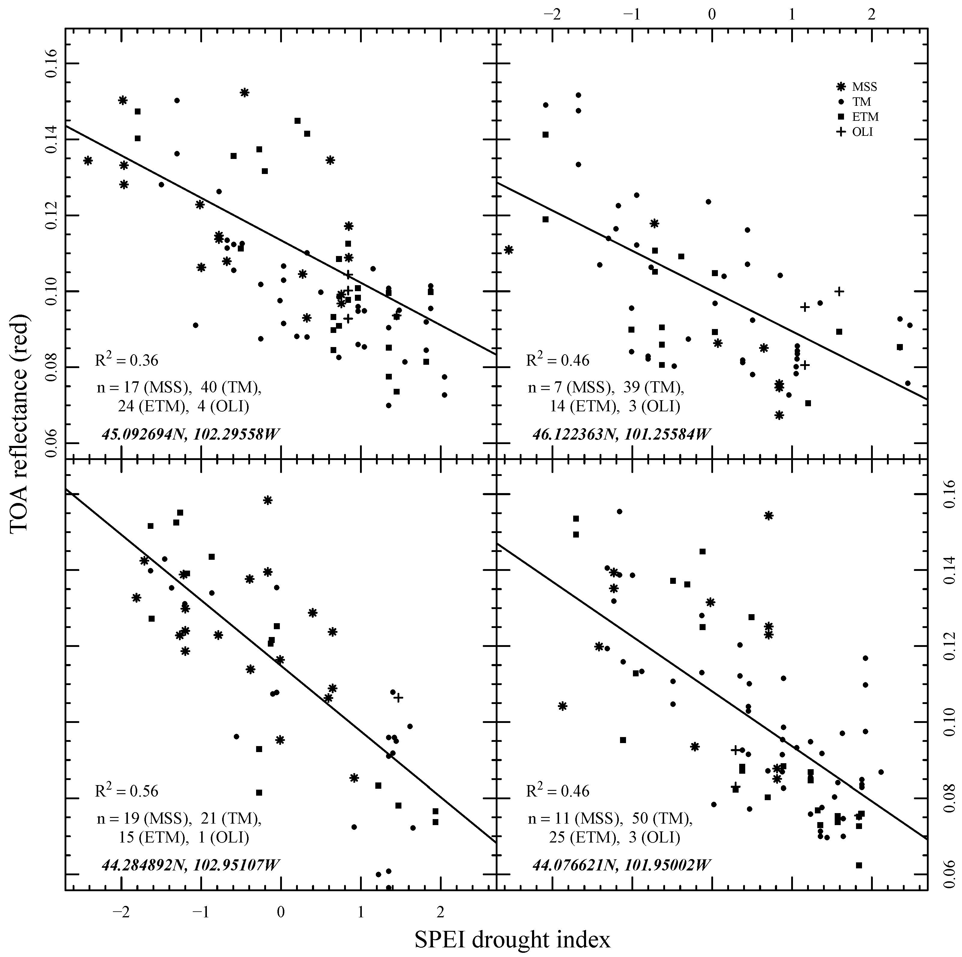
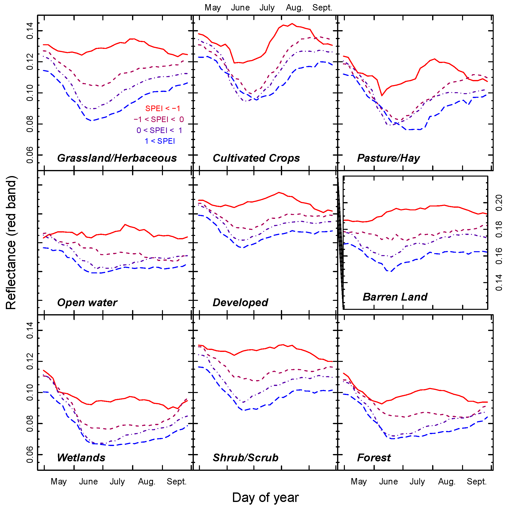
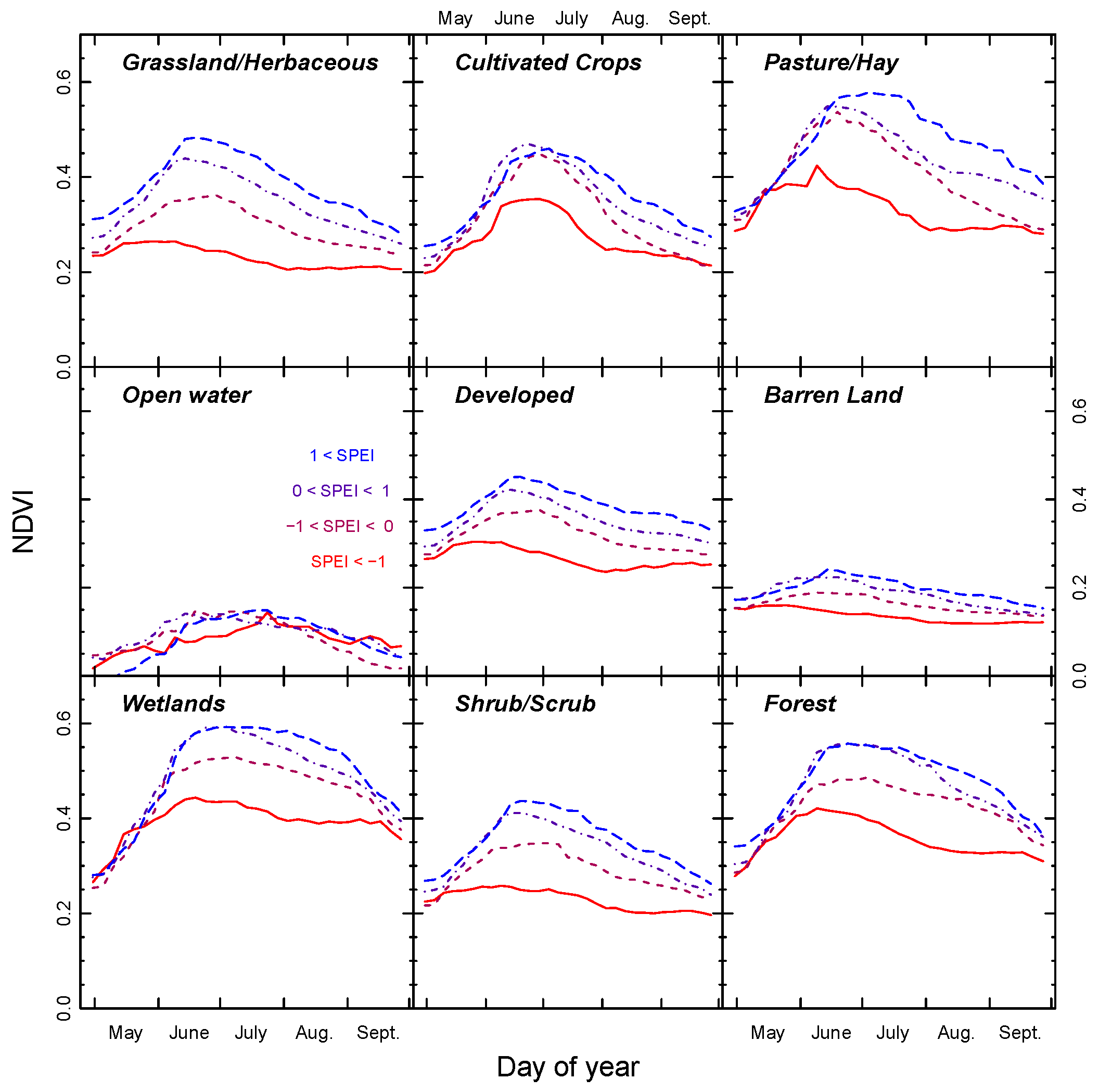
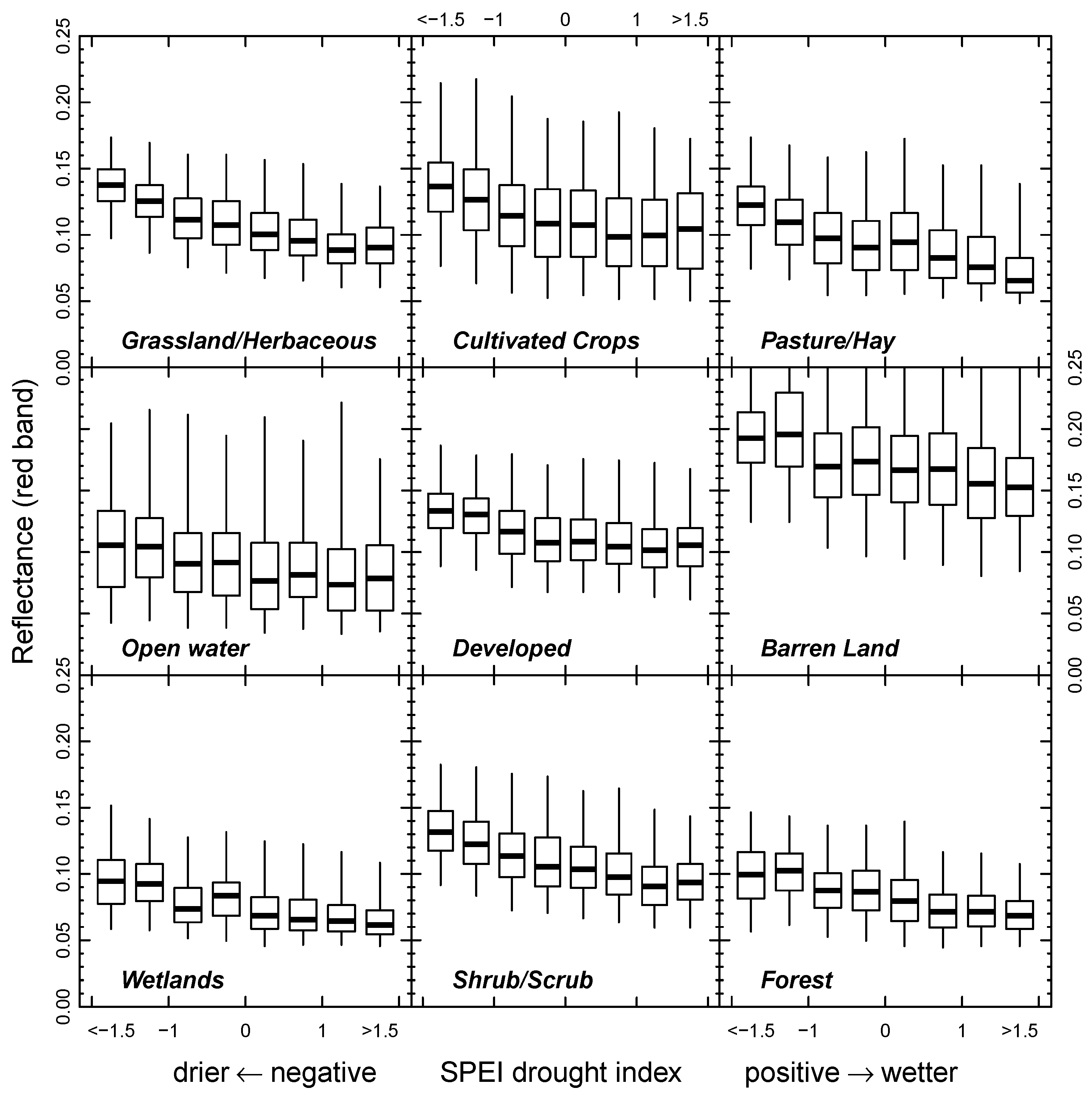
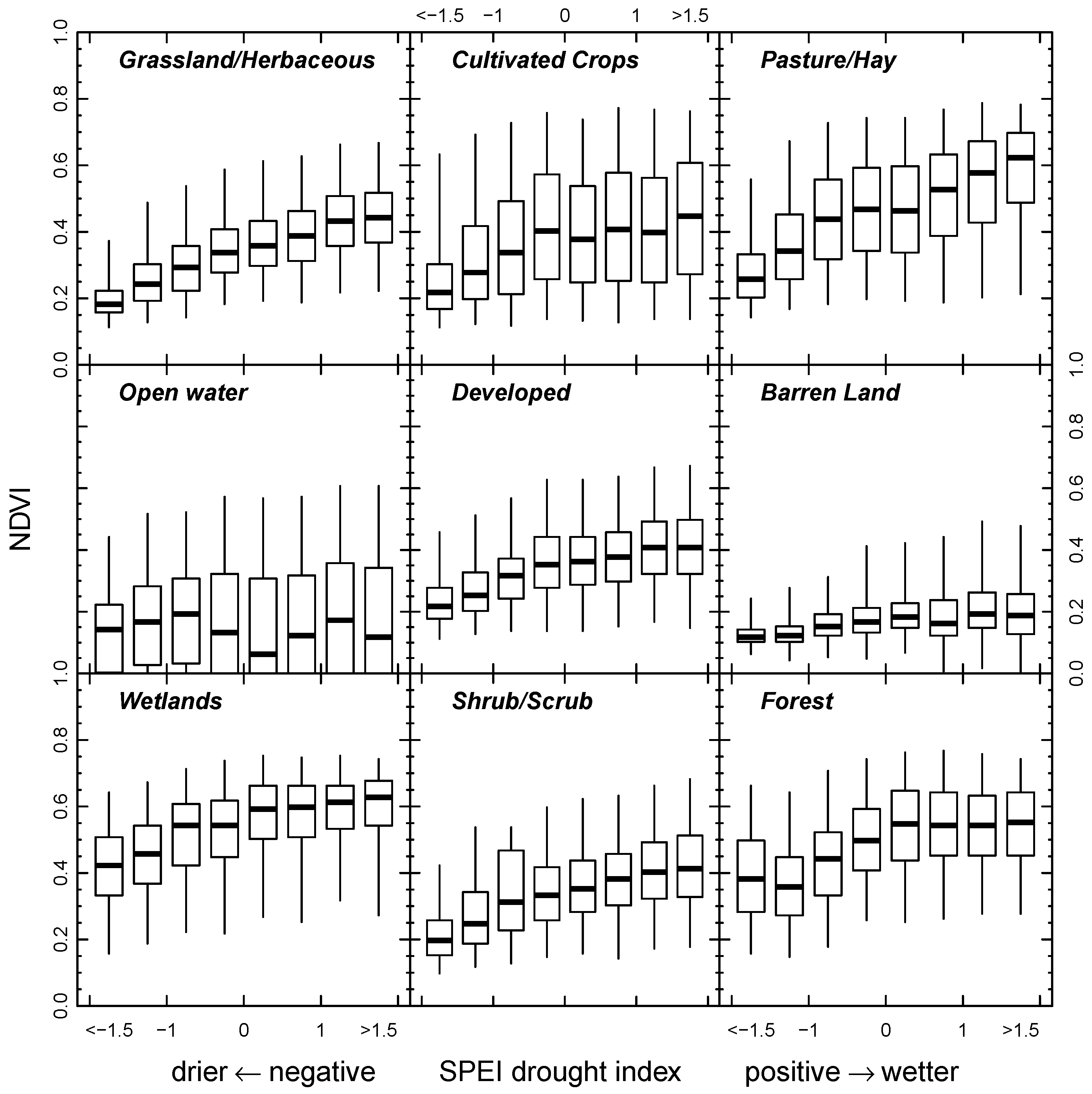
4.1. Effects of LULC and Effective Moisture on Spectral Response

Grassland, the most common LULC class in the study area (∼72% in 2011 NLCD), was observed to be highly responsive to effective moisture (Table 2). The SPEI versus red reflectance relationship had the steepest average slope (−0.014) of the classes considered, and ∼99% of grassland pixels had a significant relationship. Compared to other cover types in the study area, grassland response was also quite uniform in time and space, with an average RMSE of 0.016 for individual pixel fits and relatively small variability across the study area (Figure 9).
Cultivated crops also occurred frequently across the study area (∼17% in 2011 NLCD), but were less responsive to effective moisture and more variable than grassland. The red reflectance average slope of crops (−0.011) was lower than grassland; the mid-summer reflectance difference between dry and wet conditions was less than that found in grassland (Figure 7); and ∼62% of pixels with a significant relationship were the lowest among the LULC classes, highlighting the variability between pixels. Cropland was also variable within individual pixels, with the highest average RMSE for pixel fits (0.030). The SPEI provided less predictive power for cropland than for other categories (R 2 of 0.19); agricultural field management activities like plowing greatly affected the land surface, but did not occur at exactly the same time in every field in every year, so management decisions could have large effects on individual pixels. During the wettest periods ( SPEI > 1 ), the red reflectance minimum was delayed from mid-June to the beginning of July (Figure 9), perhaps due to late planting (for example, in years with SPEI > 1 , the median of spring wheat was ∼12% complete in the last week of April versus ∼50% in wetter years; [66]). This was one of the few times where the average reflectance during a wetter period crossed above that of a drier period.
The next most common LULC class was pasture/hay (∼6% of study area in 2011 NLCD), with results similar to crops, but with generally lower red reflectance (average intercept 0.09 versus 0.11 for crops) and higher NDVI (Figure 10). Furthermore, average RMSE (0.022) was lower than in cropland, but higher than in grassland. These observations were reasonable if well-watered land with good soil tended to become pasture where there were steeper slopes that were difficult to cultivate and tended to become cropland in large upland areas with a flatter topography.
The other LULC classes were less common in the study area (combined ∼5%, none individually >2%). Although all still had a large number of pixels (forest, with the least, had >3000), pixels of these classes tended to be more isolated (>90% of pixels in each class had a neighboring pixel of a different class) and so were more likely to be affected by sub-pixel variability and geolocation errors. Since grassland is the most common LULC class, these less common classes potentially contain substantial numbers of pixels that are partially grassland. Furthermore, these isolated pixels might not be representative of larger areas of that LULC class; for example, the riparian forest in the study area might behave differently than more extensive forested areas. However, it is still interesting to analyze these LULC categories, as they display some different patterns than the three more common classes.
Open water was the only class with a non-significant SPEI versus NDVI fit; NDVI values were near zero throughout the growing season, as expected. However, red reflectance had a shallow but significant fit (slope of −0.008). This result could be attributed to drying and water turbidity during drought, because bare soil and turbid water are more reflective than clear water. The Shadehill Reservoir (the largest water body in the study area, approximately 45°45′N, 102°15′W)) could lose more that 20% of its area during droughts [67,68], and smaller reservoirs and stockponds were likely to be even more affected by drought. Water bodies that dried out during drought were not necessarily filtered out of the dataset with the NLCD mask since none of the NLCD mapping eras (1992, 2001, 2006, and 2011) featured a serious drought in the study area (nine month SPEI showed drought in late 2006, but this late 2006 drought was not apparent in longer, e.g., two year, SPEI, and the Shadehill water levels were not especially low in 2006; [68]).
Developed land in the study area had a phenological and effective moisture response pattern similar to that of grassland, although fewer pixels had a significant relationship between effective moisture and reflectance (∼80% versus >98% for grassland). This was reasonable, since developed land is a mixture of structures, trees, and grass [54].
Barren land had by far the highest average red reflectance among the LULC types (0.17; Table 2), due to limited vegetation coverage. Unlike open water, barren land pixels tended to have low, but non-zero NDVI values; inspection of images in Google Earth showed that these pixels often contained small patches of grass or shrub. The slope of the SPEI versus red reflectance fit was fairly steep (−0.012) compared to the SPEI versus NDVI slope, suggesting that some of the reflectance relationship was due to darkening of the bare soils by moisture. This was also supported by the fairly constant value of reflectance through the summer. The high average RMSE (0.026) and low fraction of significant pixels (∼75%) demonstrated that this relationship was less well predicted for bare soil than, e.g., grassland, perhaps due partly to soil color responding more quickly than vegetation condition to precipitation.
Wetlands have a shallow red reflectance average slope (−0.008) compared to other LULC types, despite high NDVI. Wetland vegetation might be buffered due to more stable moisture availability, even during drought. A stronger response might be seen during a decadal drought (such as the 1930s). Due to their lush vegetation and the presence of water, wetlands had the lowest average red reflectance (0.077). As in the open water class, the absence of surface water during droughts might increase red reflectance. The phenology of wetlands includes a steep increase in vegetation in the spring (especially May), which is expected for the almost exclusively C 3 wetlands species, during which time, effective moisture has no apparent effect on NDVI.
The phenology curve of scrub/shrub was similar to that of grassland, with a slightly less prominent minimum in June, but with lower reflectance continuing into the fall (particularly during drought), which produced a slightly less steep red reflectance slope in the late summer period tested (−0.012; grassland: −0.014). In both grassland and scrub/shrub, the driest NDVI curve was nearly flat, with little spring green-up. In the study area, the relatively small number of scrub/shrub pixels was commonly isolated in small clusters interspersed with grassland; if these pixels often contained some grass, it was not surprising that they were similar to grassland. Shrubs tend to be deeper rooted than grass, explaining the continuation of low reflectance into the fall.
Forest was not well represented in the study area, since effective moisture was not usually high enough to support tree cover. The pixels of forest that did occur were mainly in river valleys and near watercourses. The average slope for SPEI versus red reflectance was shallow (−0.010) compared to grassland; however, pixels had low average RMSE (0.014), and most (∼99%) were significant.

4.2. Fine-Scale Spatial Variability in the Impact of Effective Moisture

The slope of the effective moisture-reflectance relationship displayed detailed patterns when shown for each 30 m pixel across space (Figure 11). Impacts of LULC were visible as expected, with grassland pixels having generally steep slopes compared to cropland, water, or forest. However, within-class variability was also visible. For example, while many bodies of water had a low slope, smaller water bodies often had a steep slope. Small water bodies in the study area could be greatly reduced in size and depth during drought, increasing their reflectance and producing a strong relationship between effective moisture and reflectance. Similarly, the Cheyenne River was notable both for carrying a substantial sediment load [69] and for having a strong effective moisture-reflectance relationship.
Patterns within grassland are of particular interest since grassland often has a strong effective moisture-reflectance relationship. For example, the Moreau Prairie ecoregion (cyan outline in Figure 11a) had lower productivity than surrounding areas because of the alkaline soils derived from the underlying Hell Creek Formation [70]. While the difference between the grassland in the Moreau Prairie and in surrounding areas was not clearly apparent in visible reflectance (Figure 11c), the central areas of the ecoregion appeared to have a less strong relationship than surrounding areas of grassland (Figure 11a). This might be attributable to lower productivity (and higher red reflectance) even in wet periods, leading to less change between wet and dry periods. Patterns in the effective moisture-reflectance relationship also followed management boundaries, topography, and soil type in some places, demonstrating that there was information available to be drawn from the slope.
The image of RMSE also displayed patterns across the land surface. Croplands stood out as locations of substantial variability, as did some bodies of water, including the Cheyenne River (visible as a dark blue line across the southern portion of the study region in Figure 11b). RMSE contained interesting within-class variability, for instance croplands commonly had high RMSE, but varied between management areas. In grasslands, one source of variability was locations having prairie dog activity at some point in the study period, which showed larger RMSE than surrounding locations.
One other advantage of this image approach was that it had the potential to highlight data inconsistencies. Although there was a sharp boundary in the SPEI values used at the half-degree latitude/longitude lines, there was little difference in slope across the boundaries (the vertical line at 102 W was due to reprojection across the UTM boundary). This suggested that the gridding of the SPEI values was not producing inconsistencies between the SPEI pixels. There was a small amount of striping due to Landsat 7 scan line corrector artifacts, and there were features at the edge of Landsat scene boundaries in the southwestern portion of the study area. However, the slope images were generally consistent between scene center and overlap zones, despite approximately double the number of observations in overlap zones and no bidirectional reflectance distribution function (BRDF) correction between the paths. In the study area, Worldwide Reference System-1 (WRS-1) overlap zones broadly covered the area of the WRS-2 scene center, so the relative observation frequency also changed through time, but was not visible in the slope or RMSE images.

5. Discussion

The relationship between effective moisture driven by weather and LULC (i.e., high visible/shortwave-IR reflectance during drought) was consistent with expectations and with previous work, e.g., [5,10,71]. During a drought, the vegetation senesces and loses its leaves, while the soil dries. These processes combine to increase visible/shortwave-IR reflectance. Near-IR reflectance is high for actively growing green vegetation and decreases with the loss of active vegetation; however, similar to visible and shortwave-IR, near-IR reflectance of dry soils tends to be high [13], suggesting that vegetation was dominating the near-IR reflectance signal. The temporal pattern was also as expected, with a larger impact from effective moisture during the growing season. Since the visible and shortwave-IR reflectance bands were observed to increase during drought, albedo could be expected to increase also, although the near-IR wavelengths would counteract this relationship.
The robustness of the relationship between effective moisture and reflectance presented here was striking; it was apparent in nearly every regional, temporal, or LULC subset that was investigated. The study area was selected as one that would likely respond to effective moisture, but even so, the wide applicability of the relationship was noteworthy. The 30 m resolution was detailed enough to show that this relationship was not just a result of averaging over a large area, but was relatively consistent across a variety of soil, vegetation, and management conditions. The magnitude of the relationship was not greatly affected by atmospheric correction, although the average reflectance did change.
The uniformity across the study area in the response of grassland to effective moisture (grassland/herbaceous in Figure 9) was quite interesting. Most of the 30 m grassland pixels in the study area responded to effective moisture in a similar way, indicating a robustness to different levels of grazing. The higher variability seen in barren land suggested that uniformity in soil reflectance was not the main driver of this uniformity and that vegetation was an important factor. Plant communities were not uniform across the study area, with variability in the fraction of C 3 and C 4 grasses [34]. This variability in vegetation suggested that different communities of grass species across the study area responded to effective moisture in a way that was broadly similar, which was potentially related to evolution in a highly variable environment with grazing pressure.
Not using time as a variable in the analysis highlighted the effective moisture-reflectance relationship by land cover type and reduced the influence of temporal biases on the analysis. For example, the full Landsat record was cross-calibrated, but if the calibration of one of the early Landsat instruments produced data that were slightly lower than that from later instruments, a time-focused analysis might find that there was an increase in reflectance even if nothing had changed on the land surface. However, the measurements from that earlier instrument would cover a range of drought index values and thus should have a more limited impact on the slope of the relationship between effective moisture and reflectance.
It is useful to note that large changes in reflectance during drought do not necessarily imply that drought is producing changes that will be long lasting or difficult to reverse once precipitation returns. For example, when grass cover senesces during drought, it can return to normal by the next growing season if precipitation returns, e.g., [72], whereas forest cover that has more stable reflectance might have substantial tree mortality due to drought, which continues to affect the character of the landscape even after the return of rain [73,74]. The strong effective moisture-reflectance relationship observed in this study suggested that much of the observed change in reflectance was reversible; if the land surface was undergoing (relatively) permanent changes during drought, then reflectance values might not return to their previous levels, and there would be more noise in the effective moisture-reflectance relationship. In a landscape that was out of equilibrium, the strong relationship found here between effective moisture and reflectance might break down, providing a potential method for locating such areas.

5.1. Potential Applications for Spatial Variability in Effective Moisture Impacts

A spatial perspective on the variability in the effective moisture-reflectance relationship potentially provides interesting tools to better delineate the characteristics of the land surface. For example, impacts related to grazing intensity might be investigated by comparing the slope between areas with different management regimes. One potentially interesting focus of study is variability between soil types, as highlighted by the Moreau Prairie ecoregion. This type of approach might provide additional information to help map small areas of differing soils, using freely available remote sensing data. Residual differences from expected values also might be used for interpreting differences through time, especially if higher resolution moisture data were available. The slope data from this study provided a time-averaged result, so that small regions of variability in the short-term (e.g., opposite sides of a field receiving different amounts of precipitation in a thunderstorm) had limited influence on the slope results.
The 30 m spatial scale allowed the possibility of detecting important patterns that might be obscured within coarser resolution satellite observations such as from Moderate Resolution Imaging Spectroradiometer (MODIS), Visible Infrared Imaging Radiometer Suite (VIIRS), or Advanced Very High Resolution Radiometer (AVHRR). For example, the difference we observed between small water bodies and their surroundings would be averaged out in imagery with coarse spatial resolution, losing the pattern of the water and reducing the slope seen in the surrounding grassland. The 30 m scale was also helpful for distinguishing patterns within classes, for example drainage patterns or irrigation features that varied within an agricultural field, or the difference in moisture response between a north- versus a south-facing slope. Even differences that were small relative to the range of variability could be observed in the slope images.

5.2. Using Reflectance and Weather Data in Modeling

Modeling of the relationship between moisture and surface reflectance in time series remote sensing data can be utilized in algorithms for change detection, e.g., [75,76]. For change detection, it is useful to understand and to be able to model processes that cause variability in satellite reflectance measurements. Quantification of the moisture-reflectance relationship has the potential to improve the ability to distinguish the effect of moisture on reflectance from other processes occurring on the land surface (e.g., clearing of land for development).
An advantage of linear regression is that it is a useful approximation that would be tractable to implement in a model of land-atmosphere feedback. In climate and weather models, albedo is often estimated based on biome and is set as a constant through time, e.g., [77,78]. To simulate feedback, albedo can be estimated from vegetation and soil fractional coverages modeled based on climate, e.g., [79]. Another approach is to utilize satellite measurements to estimate albedo, either by measuring albedo across an average year and using that for all years or in retrospective studies of recent time periods, e.g., [5,80,81]. However, it is challenging to measure albedo on near-real timescales [82] and impossible to measure albedo before the satellite record or in the future. With a simple model for the response of albedo to weather, it might become possible to improve albedo estimates beyond a constant value. Although the relationship between reflectance and effective moisture is likely to be different in other study areas and the relationship between reflectance and albedo is not straightforward, the robustness of the effective moisture-reflectance relationship presented here suggested that there was a possibility for using a drought index to model improved estimates of albedo.
Here, we modeled the relationship between effective moisture and reflectance using linear regression. Qualitatively, the plots of SPEI versus reflectance appeared to be somewhat linear (Figure 5). However, there was no mechanistic reason to assume the relationship had to be linear. In study areas less limited by water, a non-linear response is plausible; a rainforest, for example, might have increased visible reflectance (due to decreased active vegetation) in its driest periods, but not have much reflectance difference between average and wet periods (or even have decreased active vegetation causing increased reflectance during wet periods, due to less available sunlight; [83]). In any study area, reflectance cannot go beyond its theoretical bounds, and so, a linear fit must break down at extreme values of the drought index. Even within this study area, there is reason to believe that a linear relationship is only an approximation; the trend through time of pixels with SPEI < 1 is more offset than the other lines in Figure 7, and the medians of the wetter bins are roughly equal for several land cover types (e.g., cultivated crops) in Figure 9.
In addition, the simple linear regression used in this study assumed that all error was in the y-values (reflectance). This was clearly not the case, as the weather variables used in the SPEI calculation had errors, and even more importantly, converting point meteorological data to gridded data introduced significant errors. Patil [84] estimated a mean absolute error of 0.4 in SPEI for the study area due to spatial averaging. That error was similar to or larger than the 5–10% Landsat instrument errors [21]; however, surface variability will also increase the y-error. Given the extra conceptual and computational complications of a more sophisticated fit, we utilized simple linear regression, but the fit slopes would be steeper if the x-error were taken into account.
Other potential sources of error include change in LULC, the cloud mask, the use of top of atmosphere reflectance, registration, and calibration differences between instruments or over time. These errors will increase the amount of noise in the reflectance measurements, but more concerning would be if a source of error produces bias that affects the effective moisture-reflectance fit. Missed clouds during wet periods would act to decrease the slope measurement, while increased atmospheric water vapor would decrease TOA reflectance and increase the slope. The significance and robustness of the measured fit suggested that there was little cloud contamination, as thick clouds are highly reflective and would be highly significant outliers for the fit. Dust or haze in dry periods would increase the slope. Registration errors could affect pixels with subpixel or neighboring pixels with different LULC, so the uncommon LULC classes largely composed of isolated pixels were likely to be contaminated by other LULC classes (most commonly grassland). A change in LULC might also lead to incorporation of data from one class into another in this analysis, for example a pixel that was cropland early in the study period and then became grassland before 1992 would be included in the grassland data. Since time is not directly a component in the effective moisture-reflectance relationship, instrument calibration errors and other changes during the study period should not produce a large bias; any effect would be second-order (due to more droughts occurring towards the beginning of the study period). This minimization of time bias was an important advantage of using this method of analysis.

5.3. Effect of LULC on Albedo-Drought Interactions

The impact of effective moisture on reflectance can provide insight into the potential for climate-albedo feedback within different LULC categories. Since increases in albedo have been observed to reduce precipitation [5], it is important to understand albedo changes in response to effective moisture. Barren land that has a consistently high albedo, which might inhibit precipitation at all times (e.g., in the Sahara Desert), whereas grassland might be more subject to intensifying drought feedback and have large interannual precipitation variability.
The small variability in grassland visible reflectance for a given drought index shown in this study suggested that drought-albedo feedbacks were relatively predictable in grassland; albedo values would generally be similar after a given amount of effective moisture, and so should produce a similar amount of feedback. Modeling precipitation feedback might be relatively straightforward in grasslands. In contrast, the higher reflectance variability of cropland suggested that the feedback potential in cropland was not consistent throughout the study. Management decisions likely were an important part of this variability, suggesting that management could affect feedback. For example, Vick et al. [85] suggested that discontinuation of summer fallow across a large area of the northern Great Plains in recent years produced increased evapotranspiration during the summer months, leading to increased humidity and precipitation and decreased temperature. Feedback between reflectance and drought might also have importance for forest/grassland and grassland/barren transition locations.

6. Conclusions

Effective moisture had a substantial effect on reflectance across the northern U.S. Great Plains study area. Most pixels had higher visible reflectance during dry periods than during wet periods, especially in grassland, where the difference was particularly substantial. In cropland, there was more variability in reflectance at a given drought index value than in other LULC categories, although there was still a correlation between effective moisture and reflectance.
Feedbacks between albedo and moisture are an important part of the Earth system, and further research is needed to explore these interactions. The pattern of LULC on the landscape is also potentially important; boundaries between LULC types affect the initiation of convection and precipitation [86]. Using linear regression to estimate reflectance could be a helpful approach in climate models. One important topic for future consideration concerns the boundaries of LULC categories and whether feedback plays any role in maintaining these boundaries.

Supplementary Materials

The following are available at https://www.mdpi.com/2072-4292/12/12/1919/s1, Supplementary Materials S1: Landsat Scene Identifier List, Supplementary Materials S2: Reflectance Distribution As a Function of SPEI, Supplementary Materials S3: Linear Regression Results.

Author Contributions

Conceptualization, H.J.T., J.F.B., and T.R.L.; data curation, H.J.T.; formal analysis, H.J.T.; funding acquisition, H.J.T., J.F.B. and T.R.L.; investigation, H.J.T.; methodology, H.J.T.; project administration, J.F.B. and T.R.L.; resources, J.F.B. and T.R.L.; software, H.J.T.; supervision, J.F.B. and T.R.L.; validation, H.J.T.; visualization, H.J.T.; writing, original draft, H.J.T.; writing, review and editing, H.J.T., J.F.B., and T.R.L. All authors read and agreed to the published version of the manuscript.

Funding

Funding was provided by the USGS Climate and Land Use Change Mission Area. H.J.T. acknowledges the USGS Mendenhall Postdoctoral program.

Acknowledgments

We thank B.Wylie and three anonymous reviewers, whose valuable comments and suggestions improved this manuscript. The Landsat scene list and data are available in the Supplementary Materials, and cloud masks are in Tollerud [47]. Landsat data available from the U.S. Geological Survey (2016). Any use of trade, firm, or product names is for descriptive purposes only and does not imply endorsement by the U.S. Government.

Conflicts of Interest

The authors declare no conflict of interest.

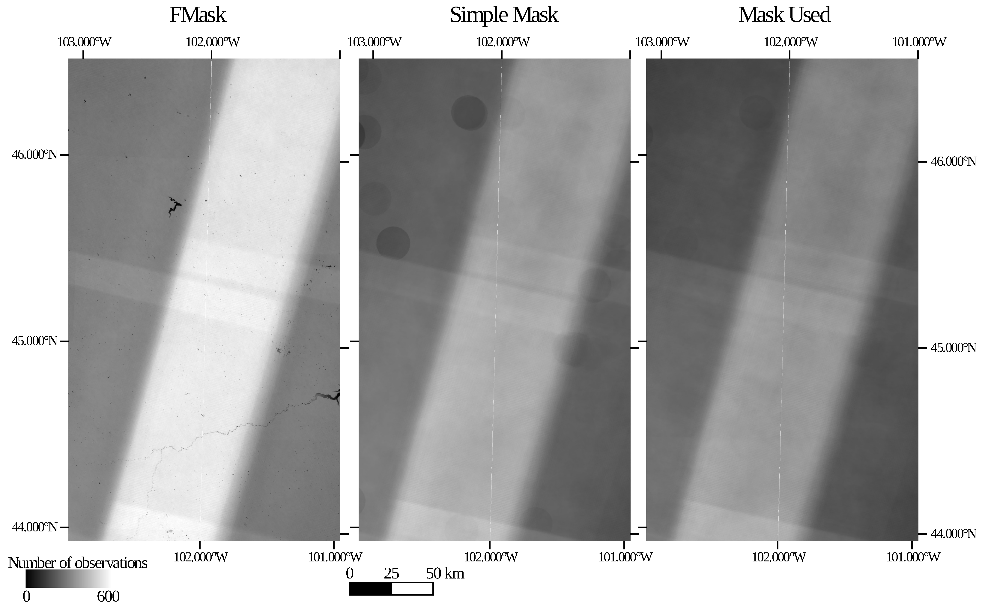
Appendix A. Cloud Masking Methods

The cloud masking goal for this study was to minimize (to the extent possible) statistical bias in the Landsat dataset due to clouds. Because clouds are highly reflective, they have substantial potential to skew data distributions; we utilized an aggressive cloud removal strategy, even at the expense of removing numerous clear pixels. This approach could be expected to remove more pixels during wet periods (when there are more clouds), but since wet periods are already expected to be less represented due to clouds, discarding some clear pixels during these periods does not add a new bias. However, areas that are consistently detected as clouds during clear conditions have the potential to produce statistical issues not already present in the data; for example, if a barren pixel is preferentially flagged during periods of high reflectivity, both its median and the slope of its relationship with the Standardized Precipitation and Evaporation Index (SPEI) would be expected to be artificially reduced. Thus, we pursued the approach of being relatively conservative in flagging pixels as clouds, but then aggressively buffered the flagged pixels to remove neighboring unflagged clouds; this approach also served to remove most cloud shadows without any other detection strategy.
The starting point for cloud masks production for this study was a simplified version of the Fmask algorithm [48]. It was also partially similar to that of Braaten et al. [49], who described a cloud mask for the Multispectral Scanner System (MSS). In the simplified algorithm, pixels are flagged as clouds if all visible bands are above a reflectance cutoff and all visible bands have a similar reflectance (since clouds tend to be uniformly bright). Cutoff values were selected manually, optimized for this study area to minimize extraneous detections seen around Badlands National Park (where highly reflective barren pixels can easily be flagged) and Rapid City, SD (the largest city near the study area). For MSS, pixels were flagged if red (R) and green (G) were both >0.35 and if G R was within (−0.02,0.025). For Thematic Mapper (TM), Enhanced Thematic Mapper Plus (ETM+), and Operational Land Imager (OLI), the test was R, G, and blue (B) all > 0.2 and both G R and B R within (−0.03,0.025). Alternately, TM, ETM+, and OLI pixels were flagged if R, G, and B were all > 0.35, since some oversaturated cloud pixels (particularly in TM) had significantly different R, G, or B values. To further reduce false detections, pixels were removed if there were not at least 10 other detected pixels in the surrounding 5 × 5 pixel region. Finally, all flagged pixels were surrounded with an aggressive buffer (20 km for MSS, 10 km for OLI/ETM+/TM), to remove undetected clouds, as well as cloud shadows.
To further reduce cloud errors and instrument artifacts (particularly in MSS), we performed a manual filtering step. The starting point was the simple cloud mask and for MSS, a mask filtering out any scan line that averaged at least twice that of surrounding lines or of the whole image. Results of Fmask (Version 3.3) were overlaid for reference during manual masking. Clouds, cloud shadows, snow, or instrument artifacts that were not detected by the simple mask were manually flagged (clear pixels in the vicinity were also flagged in the interest of analyst efficiency). False cloud detections caused by surface features were manually unmasked to reduce statistical bias (clear buffers around valid cloud detections were generally not unmasked).
The resulting dataset [47] contained a few areas with a low number of observations, but fewer than the Fmask algorithm or simple mask alone (Figure A1). The manual mask also drastically reduced the number of visible clouds in the dataset (as with any manual procedure prioritizing efficiency, there were a few misses). Manual masking also reduced haze and smoke pixels, although these were more difficult to identify and flag than clouds that were more opaque. While not done for this dataset, the simple masking procedure used as manual input could be further improved by running it a second time with the few problematic/consistently flagged pixels required to never produce cloud detections. This also might allow a slight reduction in the cutoffs used, to reduce the number of clouds missed.
Figure A1. Number of observations available at each pixel across the study area for a given masking approach. The left panel is the number of clear observations for each pixel found by the Fmask procedure. This panel does not include pixels flagged as water, but water pixels are included in the analysis. The middle panel is the result of the simple masking approach. The right panel shows the observation density after the manual masking procedure.
Remotesensing 12 01919 g0a1

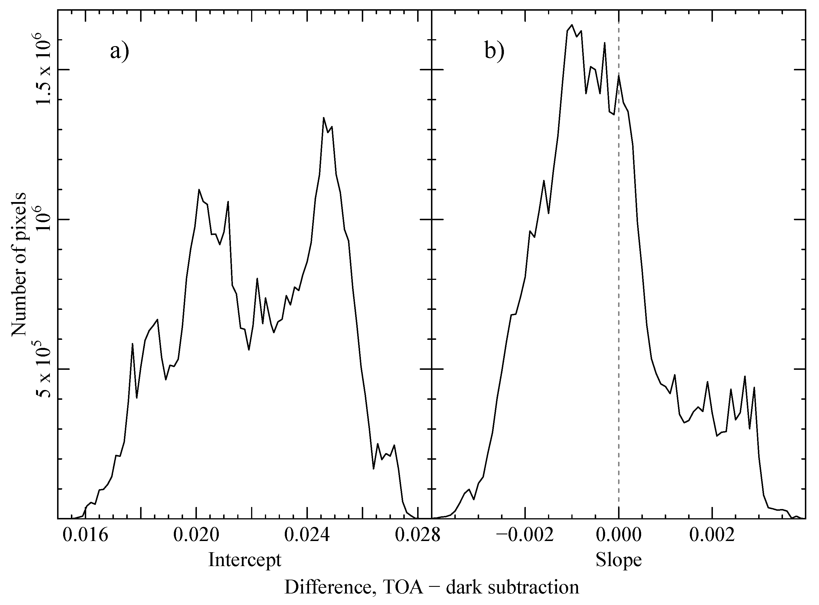
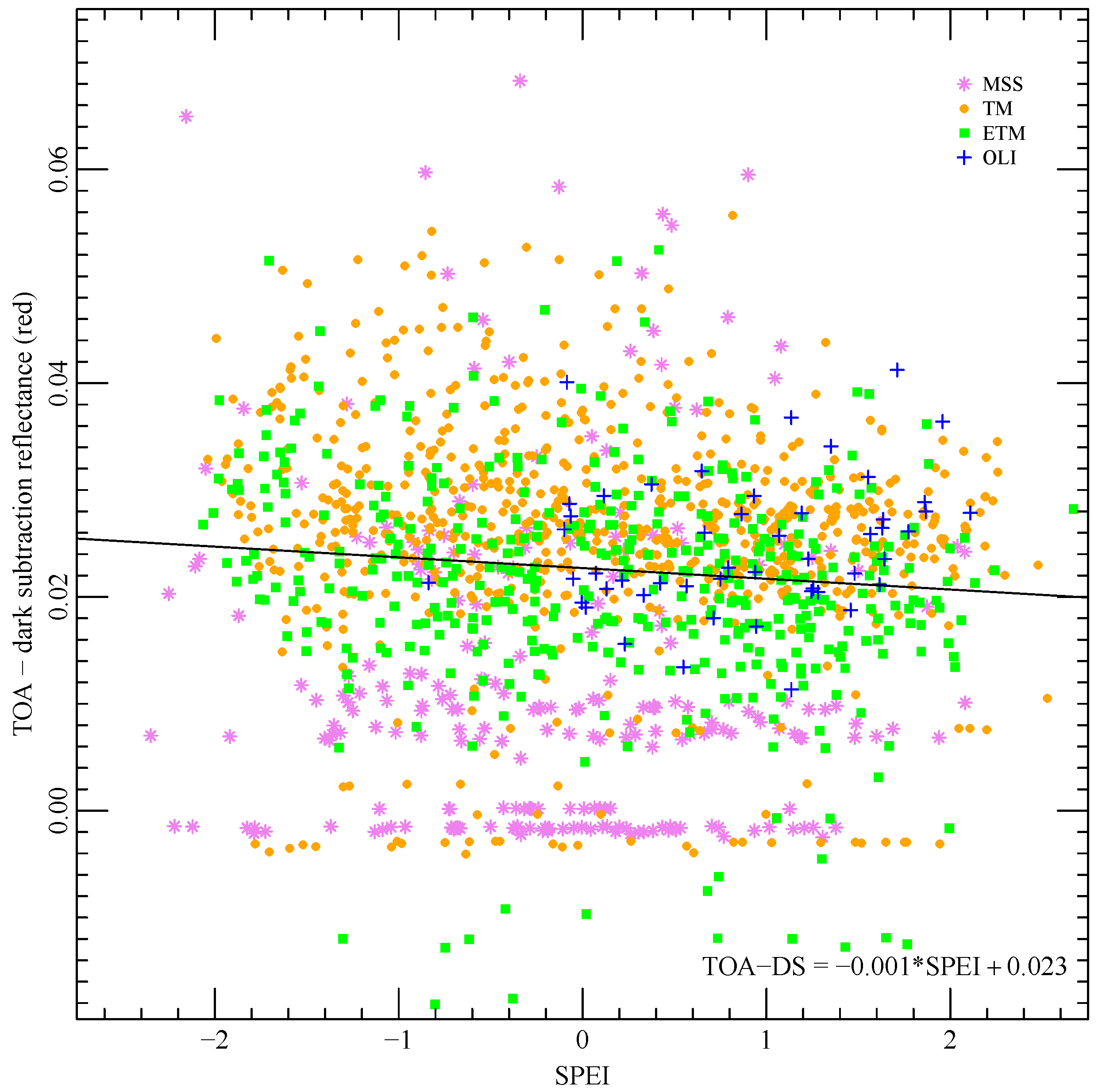
Appendix B. Atmospheric Correction with Dark Object Subtraction

We investigated the dark object subtraction method of Chavez [46] for atmospheric correction since it can be computed using MSS data. Dark object subtraction assumes that the darkest pixel(s) in an image provides an approximation of the radiance from the atmosphere, and so, subtracting that value from the image provides an atmospheric correction. Here, we focused on the red band. We found the minimum value for the red band in each Landsat observation, subtracted that from the entire image, and then converted to reflectance by multiplying by the same factor as the conversion to top of atmosphere (TOA) reflectance. Then, linear regression was performed with SPEI for all pixels, following the same method as for TOA reflectance. For each pixel in the study area, the dark subtraction linear regression intercept and slope were subtracted from the TOA intercept and slope, and then, histograms were computed across all pixels to determine how much the fit coefficients changed when the dark subtraction method was applied.
As expected, the dark subtraction correction decreased the reflectance and the SPEI-reflectance intercept (by 0.022 on average; Figure A2a). However, the effect on the slope of the SPEI-reflectance fit was small (average increase of 0.0003 compared to the average slope of −0.013; Figure A2b). This suggested that the dark subtraction correction did not have a large impact on the analysis of the SPEI-reflectance relationship.
A challenge for dark object subtraction in this study area was the lack of dark objects. Dense vegetation, deep clear water, and shadowed slopes are examples of dark targets, but none were common in the study area. Shadows from clouds are also potential dark targets, but not all observations included cloud shadows. Qualitatively, we observed that water was often the minimum used by dark object subtraction (at least in observations without cloud shadow). However, water turbidity was a potentially serious complication as it was common in the study area. In addition, we did not use the cloud masks before searching for a dark subtraction value in order to include cloud shadow as a possible source of dark subtraction. This allowed for the possibility of data artifacts producing the dark subtraction value, which we saw in some observations.
Figure A2. Histogram of the difference between TOA and dark subtraction regression coefficients for all pixels in the study area. (a) Distribution of the intercept difference (bin size = 0.00015). (b) Distribution of the slope difference (bin size = 0.0001). No difference is marked with a dashed line.
Remotesensing 12 01919 g0a2
To further investigate the relationship between dark subtraction and SPEI, we compared SPEI to the magnitude of the dark subtraction correction. For each of the 1430 Landsat observations in this study, we found the SPEI at the scene center and the difference between TOA reflectance and dark subtraction reflectance for the red band. In drier conditions (negative SPEI), the dark subtraction correction was slightly larger than during wet conditions (Figure A3). This was the opposite direction from the trend seen between SPEI and the surface reflectance correction, where the correction was larger in wet conditions (Figure 6 in the main text). It was possible that this was an accurate description of the atmospheric correction, i.e., that there was more atmospheric dust during dry periods, and so, a larger correction was needed. Alternately, it was possible that this trend was an artifact of the dark subtraction correction. If cloud shadow were more common in wet periods, the dark subtraction correction might be more accurate during wet periods and tend to produce an overcorrection during dry periods. It was also possible that the dark subtraction correction was higher due to the land surface effects we were trying to measure, or in other words, that the surface reflectance of dark targets was higher during dry periods than wet periods. Dark vegetation is likely to have higher reflectance during drought, and stock ponds, wetlands, and reservoirs are likely to have increased reflectance during drought when they become more shallow or dry completely. Thus, it would be problematic to use dark subtraction to investigate the SPEI-reflectance relationship. While it was possible that more atmospheric correction could be needed in dry conditions due to increased aerosol optical depth, it was difficult to disentangle that from the land surface effects, and the surface reflectance correction-SPEI relationship suggested that the land surface effects might be more important.
Figure A3. Comparison between SPEI and the dark subtraction (DS) correction (TOA minus dark subtraction reflectance) for the red band. Spot checks suggest that dark correction values near zero are often due to data artifacts in the Landsat observations. The black line shows the linear regression, equation ( 0.0010 ± 0.0003 ) × SPEI + ( 0.0227 ± 0.0003 ) , with p < 0.001 .
Remotesensing 12 01919 g0a3

Appendix C. Weighted Regression

Since there have been many more Landsat observations in recent years than in the early part of the record, we calculated the linear regression fits so that each year in the record would have equal weight. To do this, we weighted each observation by 1 / m i , where m i is the number of Landsat observations in the year of observation i. If the model for regression is:
y = β 0 + β 1 x + ϵ
where y is the reflectance, x is the SPEI drought index, ϵ is the residual error, and β 0 and β 1 are the fit solutions, then we maximize the likelihood L such that:
= i = 1 N ( y i ( β 0 + β 1 x i ) ) 2 m i
where N is the total number of observations. Solving for the β values,
β 1 ^ = i = 1 N y i m i j = 1 N x j m j N i = 1 N x i y i m i ( i = 1 N y i m i ) 2 N i = 1 N x i 2 m i
β 0 ^ = 1 N ( i = 1 N y i m i β 1 ^ i = 1 N x i m i ) .

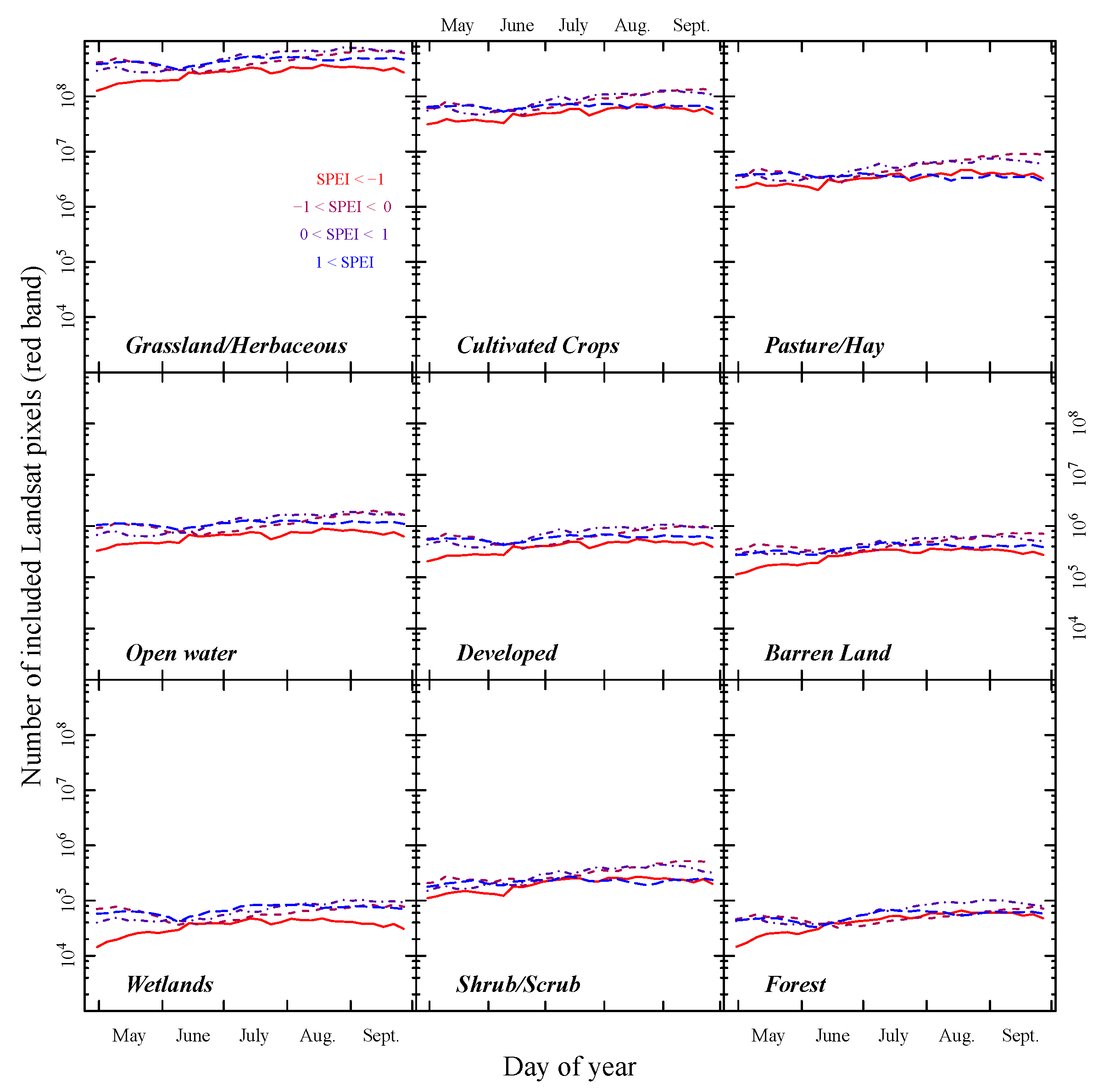
Appendix D. Count of Pixels Utilized in Summary Plots

Figure A4. Number of Landsat pixel measurements included in the figure showing average red reflectance by day of year, drought intensity, and land use/land cover (LULC). Each point on the lines shows the number of Landsat red reflectance measurements for all pixels in the study area/period that are within a 40 day window of the day of year, the specified SPEI range, and the specified LULC category. The solid red line is the driest category ( SPEI < 1 ), the short dashed maroon line drier than average (SPEI between −1 and zero), dashed dotted indigo line wetter than average (SPEI between zero and one), and dashed blue line the wettest ( SPEI > 1 ) .
Remotesensing 12 01919 g0a4

References

  1. Field, C.; Barros, V.; Mach, K.; Mastrandrea, M.; van Aalst, M.; Adger, W.; Arent, D.; Barnett, J.; Betts, R.; Bilir, T.; et al. Climate Change 2014: Impacts, Adaptation, and Vulnerability. Part A: Global and Sectoral Aspects. Contribution of Working Group II to the Fifth Assessment Report of the Intergovernmental Panel on Climate Change; Chapter Technical Summary; Cambridge University Press: Cambridge, UK; New York, NY, USA, 2014; pp. 35–94. [Google Scholar]
  2. Melillo, J.M.; Richmond, T.T.C.; Yohe, G.W. Climate Change Impacts in the United States: The Third National Climate Assessment; Technical Report; U.S. Global Change Research Program; U.S. Government Printing Office: Washington, DC, USA, 2014. [Google Scholar] [CrossRef]
  3. Loveland, T.R.; Mahmood, R. A Design for a Sustained Assessment of Climate Forcing and Feedbacks Related to Land Use and Land Cover Change. Bull. Am. Meteorol. Soc. 2014. [Google Scholar] [CrossRef]
  4. Mahmood, R.; Pielke, R.A.; Hubbard, K.G.; Niyogi, D.; Dirmeyer, P.A.; McAlpine, C.; Carleton, A.M.; Hale, R.; Gameda, S.; Beltrán-Przekurat, A.; et al. Land cover changes and their biogeophysical effects on climate. Int. J. Climatol. 2014, 34, 929–953. [Google Scholar] [CrossRef]
  5. Meng, X.H.; Evans, J.P.; McCabe, M.F. The influence of inter-annually varying albedo on regional climate and drought. Clim. Dyn. 2014, 42, 787–803. [Google Scholar] [CrossRef]
  6. Ji, L.; Peters, A.J. Assessing vegetation response to drought in the northern Great Plains using vegetation and drought indices. Remote Sens. Environ. 2003, 87, 85–98. [Google Scholar] [CrossRef]
  7. Govaerts, Y.; Lattanzio, A. Estimation of surface albedo increase during the eighties Sahel drought from Meteosat observations. Glob. Planet. Chang. 2008, 64, 139–145. [Google Scholar] [CrossRef]
  8. Wang, J.; Rich, P.M.; Price, K.P. Temporal responses of NDVI to precipitation and temperature in the central Great Plains, USA. Int. J. Remote Sens. 2010, 24, 2345–2364. [Google Scholar] [CrossRef]
  9. Yu, F.; Price, K.P.; Ellis, J.; Feddema, J.J.; Shi, P. Interannual variations of the grassland boundaries bordering the eastern edges of the Gobi Desert in central Asia. Int. J. Remote Sens. 2004, 25, 327–346. [Google Scholar] [CrossRef]
  10. Vicente-Serrano, S.M.; Gouveia, C.; Camarero, J.J.; Beguería, S.; Trigo, R.; López-Moreno, J.I.; Azorín-Molina, C.; Pasho, E.; Lorenzo-Lacruz, J.; Revuelto, J.; et al. Response of vegetation to drought time-scales across global land biomes. Proc. Natl. Acad. Sci. USA 2013, 110, 52–57. [Google Scholar] [CrossRef] [Green Version]
  11. Brown, J.F.; Wardlow, B.D.; Tadesse, T.; Hayes, M.J.; Reed, B.C. The Vegetation Drought Response Index (VegDRI): A New Integrated Approach for Monitoring Drought Stress in Vegetation. GISci. Remote Sens. 2008, 45, 16–46. [Google Scholar] [CrossRef]
  12. Karnieli, A.; Agam, N.; Pinker, R.T.; Anderson, M.; Imhoff, M.L.; Gutman, G.G.; Panov, N.; Goldberg, A. Use of NDVI and Land Surface Temperature for Drought Assessment: Merits and Limitations. J. Clim. 2010, 23, 618–633. [Google Scholar] [CrossRef]
  13. Liu, W.; Baret, F.; Gu, X.; Tong, Q.; Zheng, L.; Zhang, B. Relating soil surface moisture to reflectance. Remote Sens. Environ. 2002, 81, 238–246. [Google Scholar] [CrossRef]
  14. Fan, X.; Ma, Z.; Yang, Q.; Han, Y.; Mahmood, R. Land use/land cover changes and regional climate over the Loess Plateau during 2001–2009. Part II: Interrelationship from observations. Clim. Chang. 2015, 129, 441–455. [Google Scholar] [CrossRef] [Green Version]
  15. Baldocchi, D.D.; Xu, L.; Kiang, N. How plant functional-type, weather, seasonal drought, and soil physical properties alter water and energy fluxes of an oak–grass savanna and an annual grassland. Agric. For. Meteorol. 2004, 123, 13–39. [Google Scholar] [CrossRef] [Green Version]
  16. Zha, T.; Barr, A.G.; van der Kamp, G.; Black, T.A.; McCaughey, J.H.; Flanagan, L.B. Interannual variation of evapotranspiration from forest and grassland ecosystems in western Canada in relation to drought. Agric. For. Meteorol. 2010, 150, 1476–1484. [Google Scholar] [CrossRef]
  17. Fraser, E.D.; Simelton, E.; Termansen, M.; Gosling, S.N.; South, A. “Vulnerability hotspots”: Integrating socio-economic and hydrological models to identify where cereal production may decline in the future due to climate change induced drought. Agric. For. Meteorol. 2013, 170, 195–205. [Google Scholar] [CrossRef]
  18. Roy, D.; Wulder, M.; Loveland, T.; Woodcock, C.E.; Allen, R.; Anderson, M.; Helder, D.; Irons, J.; Johnson, D.; Kennedy, R.; et al. Landsat-8: Science and product vision for terrestrial global change research. Remote Sens. Environ. 2014, 145, 154–172. [Google Scholar] [CrossRef] [Green Version]
  19. Pasquarella, V.J.; Holden, C.E.; Kaufman, L.; Woodcock, C.E. From imagery to ecology: Leveraging time series of all available Landsat observations to map and monitor ecosystem state and dynamics. Remote Sens. Ecol. Conser. 2016, 2, 152–170. [Google Scholar] [CrossRef]
  20. Wulder, M.A.; Hilker, T.; White, J.C.; Coops, N.C.; Masek, J.G.; Pflugmacher, D.; Crevier, Y. Virtual constellations for global terrestrial monitoring. Remote Sens. Environ. 2015, 170, 62–76. [Google Scholar] [CrossRef] [Green Version]
  21. Markham, B.L.; Helder, D.L. Forty-year calibrated record of earth-reflected radiance from Landsat: A review. Remote Sens. Environ. 2012, 122, 30–40. [Google Scholar] [CrossRef] [Green Version]
  22. Hernandez, E.A.; Uddameri, V. Standardized precipitation evaporation index (SPEI)-based drought assessment in semi-arid south Texas. Environ. Earth Sci. 2014, 71, 2491–2501. [Google Scholar] [CrossRef]
  23. Vicente-Serrano, S.M.; Beguería, S.; López-Moreno, J.I. A Multiscalar Drought Index Sensitive to Global Warming: The Standardized Precipitation Evapotranspiration Index. J. Clim. 2010, 23, 1696–1718. [Google Scholar] [CrossRef] [Green Version]
  24. Beguería, S.; Vicente-Serrano, S.M.; Reig, F.; Latorre, B. Standardized precipitation evapotranspiration index (SPEI) revisited: Parameter fitting, evapotranspiration models, tools, datasets and drought monitoring. Int. J. Climatol. 2014, 34, 3001–3023. [Google Scholar] [CrossRef] [Green Version]
  25. Vicente-Serrano, S.M.; der Schrier, G.V.; Beguería, S.; Azorin-Molina, C.; Lopez-Moreno, J.I. Contribution of precipitation and reference evapotranspiration to drought indices under different climates. J. Hydrol. 2015, 526, 42–54. [Google Scholar] [CrossRef] [Green Version]
  26. White, A.B.; Kumar, P.; Tcheng, D. A data mining approach for understanding topographic control on climate-induced inter-annual vegetation variability over the United States. Remote Sens. Environ. 2005, 98, 1–20. [Google Scholar] [CrossRef]
  27. Hoerling, M.; Eischeid, J.; Kumar, A.; Leung, R.; Mariotti, A.; Mo, K.; Schubert, S.; Seager, R.; Hoerling, M.; Eischeid, J.; et al. Causes and Predictability of the 2012 Great Plains Drought. Bull. Am. Meteorol. Soc. 2014, 95, 269–282. [Google Scholar] [CrossRef] [Green Version]
  28. Gibson, D.J. Grasses and Grassland Ecology; Oxford University Press: Oxford, UK, 2009; Volume 104, p. ix. [Google Scholar] [CrossRef] [Green Version]
  29. Arguez, A.; Durre, I.; Applequist, S.; Squires, M.; Vose, R.; Yin, X.; Bilotta, R. NOAA’s U.S. Climate Normals (1981–2010). Dataset. 2010. Available online: https://doi.org/10.7289/V5PN93JP (accessed on 29 April 2020).
  30. NOAA NCEI. U.S. Billion-Dollar Weather and Climate Disasters. Dataset. 2017. Available online: www.ncdc.noaa.gov/billions/ (accessed on 29 April 2020).
  31. Homer, C.; Dewitz, J.; Fry, J.; Coan, M.; Hossain, N.; Larson, C.; Herold, N.; McKerrow, A.; VanDriel, J.N.; Wickham, J.; et al. Completion of the 2001 national land cover database for the counterminous United States. Photogramm. Eng. Remote Sens. 2007, 73, 337. [Google Scholar]
  32. U.S. Department of Agriculture. 2012 Census of Agriculture; Technical Report AC-12-A-51; National Agricultural Statistics Service, U.S. Department of Agriculture: Washington, DC, USA, 2014.
  33. Greer, M.J.; Bakker, K.K.; Dieter, C.D. Grassland bird response to recent loss and degradation of native prairie in central and western South Dakota. Wilson J. Ornithol. 2016, 128, 278–289. [Google Scholar] [CrossRef] [Green Version]
  34. Tieszen, L.L.; Reed, B.C.; Bliss, N.B.; Wylie, B.K.; DeJong, D.D. NDVI, C3 and C4 production, and distributions in Great Plains grassland land cover classes. Ecol. Appl. 1997, 7, 59–78. [Google Scholar] [CrossRef]
  35. U.S. Department of Agriculture. 2014 Cropland Data Layer. Dataset. 2015. Available online: nassgeodata.gmu.edu/CropScape/ (accessed on 29 April 2020).
  36. U.S. Department of Agriculture. Field Crops Usual Planting and Harvesting Dates; Technical Report; United States Department of Agriculture National Agricultural Statistics Service: Washington, DC, USA, 2010; Agricultural Handbook Number 628.
  37. U.S. Department of Agriculture. 2007 Census of Agriculture, South Dakota State and County Data; Technical Report AC-07-A-41; National Agricultural Statistics Service, U.S. Department of Agriculture: Washington, DC, USA, 2009; Map 07-M082.
  38. Whitehead, R. Ground Water Atlas of the United States: Segment 8, Montana, North Dakota, South Dakota, Wyoming; Technical Report 730-I; U.S. Geological Survey: Reston, VA, USA, 1996.
  39. Taylor, J.L.; Acevedo, W.; Auch, R.F.; Drummond, M.A. Status and Trends of Land Change in the Western United States–1973 to 2000: U.S. Geological Survey Professional Paper 1794–B; Technical Report; US Department of the Interior, US Geological Survey: Reston, VA, USA, 2015. [CrossRef] [Green Version]
  40. U.S. Department of Agriculture. Conservation Reserve Program Statistics. Dataset. 2017. Available online: www.fsa.usda.gov/programs-and-services/conservation-programs/reports-and-statistics/conservation-reserve-program-statistics/index (accessed on 29 April 2020).
  41. Townshend, J.R.; Masek, J.G.; Huang, C.; Vermote, E.F.; Gao, F.; Channan, S.; Sexton, J.O.; Feng, M.; Narasimhan, R.; Kim, D.; et al. Global characterization and monitoring of forest cover using Landsat data: Opportunities and challenges. Int. J. Digit. Earth 2012, 5, 373–397. [Google Scholar] [CrossRef] [Green Version]
  42. U.S. Geological Survey. Landsat Data Archive. Dataset. 2016. Available online: www.usgs.gov/centers/eros (accessed on 29 April 2020).
  43. Wulder, M.A.; White, J.C.; Loveland, T.R.; Woodcock, C.E.; Belward, A.S.; Cohen, W.B.; Fosnight, E.A.; Shaw, J.; Masek, J.G.; Roy, D.P. The global Landsat archive: Status, consolidation, and direction. Remote Sens. Environ. 2016, 185, 271–283. [Google Scholar] [CrossRef] [Green Version]
  44. Masek, J.G.; Vermote, E.F.; Saleous, N.E.; Wolfe, R.; Hall, F.G.; Huemmrich, K.F.; Kutler, J. A Landsat surface reflectance dataset for North America, 1990–2000. IEEE Geosci. Remote Sens. Lett. 2006, 3, 68–72. [Google Scholar] [CrossRef]
  45. Vermote, E.; Justice, C.; Claverie, M.; Franch, B. Preliminary analysis of the performance of the Landsat 8/OLI land surface reflectance product. Remote Sens. Environ. 2016, 185, 46–56, Landsat 8 Science Results. [Google Scholar] [CrossRef] [PubMed]
  46. Chavez, P.S. An improved dark-object subtraction technique for atmospheric scattering correction of multispectral data. Remote Sens. Environ. 1988, 24, 459–479. [Google Scholar] [CrossRef]
  47. Tollerud, H. Landsat Cloud Masks in Western South Dakota; U.S. Geological Survey: Reston, VA, USA, 2019. [CrossRef]
  48. Zhu, Z.; Woodcock, C.E. Object-based cloud and cloud shadow detection in Landsat imagery. Remote Sens. Environ. 2012, 118, 83–94. [Google Scholar] [CrossRef]
  49. Braaten, J.D.; Cohen, W.B.; Yang, Z. Automated cloud and cloud shadow identification in Landsat MSS imagery for temperate ecosystems. Remote Sens. Environ. 2015, 169, 128–138. [Google Scholar] [CrossRef] [Green Version]
  50. Storey, J.; Choate, M. Landsat-5 bumper-mode geometric correction. IEEE Trans. Geosci. Remote Sens. 2004, 42, 2695–2703. [Google Scholar] [CrossRef]
  51. U.S. Geological Survey. Landsat 7 (L7) Data Users Handbook; Technical Report LSDS-1927; U.S. Geological Survey: Sioux Falls, SD, USA, 2018.
  52. Vicente-Serrano, S.M.; Beguería, S. Global SPEI Database, SPEIbase. Dataset, Version 2.4, Based on CRU TS 3.23. 2016. Available online: http://digital.csic.es/handle/10261/128892 (accessed on 29 April 2020).
  53. Harris, I.; Jones, P.; Osborn, T.; Lister, D. Updated high-resolution grids of monthly climatic observations—The CRU TS3.10 Dataset. Int. J. Climatol. 2014, 34, 623–642. [Google Scholar] [CrossRef] [Green Version]
  54. Multi-Resolution Land Characteristics Consortium. National Land Cover Database. Dataset. 2011. Available online: www.mrlc.gov (accessed on 29 April 2020).
  55. Wickham, J.; Stehman, S.V.; Gass, L.; Dewitz, J.A.; Sorenson, D.G.; Granneman, B.J.; Poss, R.V.; Baer, L.A. Thematic accuracy assessment of the 2011 National Land Cover Database (NLCD). Remote Sens. Environ. 2017, 191, 328–341. [Google Scholar] [CrossRef] [Green Version]
  56. Vogelmann, J.E.; Howard, S.M.; Yang, L.; Larson, C.R.; Wylie, B.K.; Van Driel, N. Completion of the 1990s National Land Cover Data Set for the conterminous United States from Landsat Thematic Mapper data and ancillary data sources. Photogramm. Eng. Remote Sens. 2001, 67, 650–662. [Google Scholar]
  57. Fry, J.; Xian, G.; Jin, S.; Dewitz, J.; Homer, C.; Yang, L.; Barnes, C.; Herold, N.; Wickham, J. Completion of the 2006 national land cover database for the conterminous united states. Photogramm. Eng. Remote Sens. 2011, 77, 858–864. [Google Scholar]
  58. Homer, C.G.; Dewitz, J.A.; Yang, L.; Jin, S.; Danielson, P.; Xian, G.; Coulston, J.; Herold, N.D.; Wickham, J.; Megown, K. Completion of the 2011 National Land Cover Database for the conterminous United States-Representing a decade of land cover change information. Photogramm. Eng. Remote Sens. 2015, 81, 345–354. [Google Scholar]
  59. Huang, W.; Huang, J.; Wang, X.; Wang, F.; Shi, J. Comparability of Red/Near-Infrared Reflectance and NDVI Based on the Spectral Response Function between MODIS and 30 Other Satellite Sensors Using Rice Canopy Spectra. Sensors 2013, 13, 16023–16050. [Google Scholar] [CrossRef] [PubMed]
  60. Roy, D.; Kovalskyy, V.; Zhang, H.; Vermote, E.; Yan, L.; Kumar, S.; Egorov, A. Characterization of Landsat-7 to Landsat-8 reflective wavelength and normalized difference vegetation index continuity. Remote Sens. Environ. 2016, 185, 57–70. [Google Scholar] [CrossRef] [PubMed] [Green Version]
  61. Fuller, W.A.; Hidiroglou, M.A. Regression Estimation After Correcting for Attenuation. J. Am. Stat. Assoc. 1978, 73, 99–104. [Google Scholar] [CrossRef]
  62. R Core Team. R: A Language and Environment for Statistical Computing; R Foundation for Statistical Computing: Vienna, Austria, 2015. [Google Scholar]
  63. QGIS Development Team. QGIS Geographic Information System; Open Source Geospatial Foundation Project; QGIS Development Team, 2016; Available online: http://qgis.org (accessed on 29 April 2020).
  64. Ollinger, S.V. Sources of variability in canopy reflectance and the convergent properties of plants. New Phytol. 2011, 189, 375–394. [Google Scholar] [CrossRef]
  65. Rigge, M.; Smart, A.; Wylie, B.; Gilmanov, T.; Johnson, P. Linking Phenology and Biomass Productivity in South Dakota Mixed-Grass Prairie. Rangel. Ecol. Manag. 2013, 66, 579–587. [Google Scholar] [CrossRef] [Green Version]
  66. U.S. Department of Agriculture. Weekly Weather and Crop Bulletin. 2016. Available online: usda.mannlib.cornell.edu/MannUsda/viewDocumentInfo.do?documentID=1393 (accessed on 29 April 2020).
  67. Ferrari, R.L. Shadehill Reservoir 1993 Sedimentation Survey. Technical Report, Bureau of Reclamation, Technical Service Center Denver CO 80225. 1995. Available online: www.usbr.gov/tsc/techreferences/reservoir/ShadehillReservoir1993SedimentationSurvey.pdf (accessed on 29 April 2020).
  68. U.S. Bureau of Reclamation. Shadehill Monthly Reservoir Elevation 1952–2016. Dataset; V2.6, retrieved 1/2017; U.S. Bureau of Reclamation: Washington, DC, USA, 1997.
  69. Callender, E.; Robbins, J.A. Transport and accumulation of radionuclides and stable elements in a Missouri River Reservoir. Water Resour. Res. 1993, 29, 1787–1804. [Google Scholar] [CrossRef]
  70. Bryce, S.; Omernik, J.; Pater, D.; Ulmer, M.; Schaar, J.; Freeouf, J.; Johnson, R.; Kuck, P.; Azevedo, S. Ecoregions of North Dakota and South Dakota. Color Poster with Map, Descriptive Text, Summary Tables, and Photographs; Map scale 1:1,500,000; U.S. Geological Survey: Reston, VA, USA, 1996.
  71. Krishnan, P.; Meyers, T.P.; Scott, R.L.; Kennedy, L.; Heuer, M. Energy exchange and evapotranspiration over two temperate semi-arid grasslands in North America. Agric. For. Meteorol. 2012, 153, 31–44. [Google Scholar] [CrossRef]
  72. Hoover, D.L.; Knapp, A.K.; Smith, M.D. Resistance and resilience of a grassland ecosystem to climate extremes. Ecology 2014, 95, 2646–2656. [Google Scholar] [CrossRef] [Green Version]
  73. Allen, C.D.; Macalady, A.K.; Chenchouni, H.; Bachelet, D.; McDowell, N.; Vennetier, M.; Kitzberger, T.; Rigling, A.; Breshears, D.D.; Hogg, E.T.; et al. A global overview of drought and heat-induced tree mortality reveals emerging climate change risks for forests. For. Ecol. Manag. 2010, 259, 660–684. [Google Scholar] [CrossRef] [Green Version]
  74. Vose, J.M.; Clark, J.S.; Luce, C.H.; Patel-Weynand, T. Effects of Drought on Forests and Rangelands in the United States: A Comprehensive Science Synthesis; Technical Report Gen. Tech. Report WO-93b; Forest Service Research & Development: Washington, DC, USA, 2016. [CrossRef] [Green Version]
  75. Zhu, Z.; Woodcock, C.E. Continuous change detection and classification of land cover using all available Landsat data. Remote Sens. Environ. 2014, 144, 152–171. [Google Scholar] [CrossRef] [Green Version]
  76. Brown, J.F.; Tollerud, H.J.; Barber, C.P.; Zhou, Q.; Dwyer, J.L.; Vogelmann, J.E.; Loveland, T.R.; Woodcock, C.E.; Stehman, S.V.; Zhu, Z.; et al. Lessons learned implementing an operational continuous United States national land change monitoring capability: The Land Change Monitoring, Assessment, and Projection (LCMAP) approach. Remote Sens. Environ. 2020, 238, 111356. [Google Scholar] [CrossRef]
  77. Chikira, M.; Abe-Ouchi, A.; Sumi, A. General circulation model study on the green Sahara during the mid-Holocene: An impact of convection originating above boundary layer. J. Geophys. Res. Atmos. 2006, 111. [Google Scholar] [CrossRef]
  78. Pausata, F.S.; Messori, G.; Zhang, Q. Impacts of dust reduction on the northward expansion of the African monsoon during the Green Sahara period. Earth Planet. Sci. Lett. 2016, 434, 298–307. [Google Scholar] [CrossRef] [Green Version]
  79. Vamborg, F.; Brovkin, V.; Claussen, M. The effect of a dynamic background albedo scheme on Sahel/Sahara precipitation during the mid-Holocene. Clim. Past 2011, 7, 117–131. [Google Scholar] [CrossRef] [Green Version]
  80. Zaitchik, B.F.; Evans, J.P.; Geerken, R.A.; Smith, R.B.; Zaitchik, B.F.; Evans, J.P.; Geerken, R.A.; Smith, R.B. Climate and Vegetation in the Middle East: Interannual Variability and Drought Feedbacks. J. Clim. 2007, 20, 3924–3941. [Google Scholar] [CrossRef]
  81. Rechid, D.; Raddatz, T.J.; Jacob, D. Parameterization of snow-free land surface albedo as a function of vegetation phenology based on MODIS data and applied in climate modelling. Theor. Appl. Climatol. 2009, 95, 245–255. [Google Scholar] [CrossRef] [Green Version]
  82. Boussetta, S.; Balsamo, G.; Dutra, E.; Beljaars, A.; Albergel, C. Assimilation of surface albedo and vegetation states from satellite observations and their impact on numerical weather prediction. Remote Sens. Environ. 2015, 163, 111–126. [Google Scholar] [CrossRef] [Green Version]
  83. Restrepo-Coupe, N.; da Rocha, H.R.; Hutyra, L.R.; da Araujo, A.C.; Borma, L.S.; Christoffersen, B.; Cabral, O.M.; de Camargo, P.B.; Cardoso, F.L.; da Costa, A.C.L.; et al. What drives the seasonality of photosynthesis across the Amazon basin? A cross-site analysis of eddy flux tower measurements from the Brasil flux network. Agric. For. Meteorol. 2013, 182-183, 128–144. [Google Scholar] [CrossRef] [Green Version]
  84. Patil, S. Analysis of Spatial Performance of Meteorological Drought Indices. Master’s Thesis, Texas A&M University, College Station, TX, USA, 2013. Available online: http://hdl.handle.net/1969.1/148327 (accessed on 29 April 2020).
  85. Vick, E.S.; Stoy, P.C.; Tang, A.C.; Gerken, T. The surface-atmosphere exchange of carbon dioxide, water, and sensible heat across a dryland wheat-fallow rotation. Agric. Ecosyst. Environ. 2016, 232, 129–140. [Google Scholar] [CrossRef] [Green Version]
  86. Carleton, A.M.; Travis, D.J.; Adegoke, J.O.; Arnold, D.L.; Curran, S.; Carleton, A.M.; Travis, D.J.; Adegoke, J.O.; Arnold, D.L.; Curran, S. Synoptic Circulation and Land Surface Influences on Convection in the Midwest U.S. “Corn Belt” during the Summers of 1999 and 2000. Part II: Role of Vegetation Boundaries. J. Clim. 2008, 21, 3617–3641. [Google Scholar] [CrossRef]
Figure 1. The location of the study area in the western Dakotas (yellow box) shown over a Landsat natural color mosaic of late summer (Landsat 8; July 15–Aug 15; 2013–2016). The four main Landsat scenes used in this study are outlined with dotted grey lines. The filtered National Land Cover Database for the study area is shown in the panel in the upper right (black = not used for this study, tan = grassland, dark brown = crops, yellow = pasture/hay, blue = water).
Remotesensing 12 01919 g001
Figure 2. Average of precipitation and temperature for meteorological stations within the study area. Bars show monthly average precipitation, and lines show average minimum and maximum daily temperatures. Data from Arguez et al. [29].
Remotesensing 12 01919 g002
Figure 3. Landsat red reflectance through time for one grassland pixel (45°5′33.7″N, 102°17′44.1″W). Colors denote the Standardized Precipitation and Evaporation Index (SPEI) value at the observation time (red = dry, blue = wet). Landsat instrument shown by symbols: MSS (asterisk), TM (circle), ETM (square), and OLI (plus).
Remotesensing 12 01919 g003
Figure 4. The record of 9 month SPEI in the study area. The grey area shows the range of SPEI covered by the 20 half-degree SPEI pixels within the study area; the black line is the average value for the 20 pixels.
Remotesensing 12 01919 g004
Figure 5. Example pixel fits of SPEI versus red Landsat reflectance for observations during Day of Year 180–220 (∼July). All four example pixels are from unmixed areas classified as grassland throughout the study period.
Remotesensing 12 01919 g005
Figure 6. SPEI versus the mean difference of TOA minus surface reflectance (SR) for 90 Landsat observations for the red band. Note that the range in reflectance difference is ∼0.015, compared to a range of ∼0.1 in Figure 5. The grey lines show one standard deviation around the mean difference. The black line is the regression fit. Orange circles are TM observations, green squares ETM+, and blue pluses OLI.
Remotesensing 12 01919 g006
Figure 7. Average red reflectance by day of year, drought intensity, and LULC. Each point on the lines shows the average red reflectance for all pixels in the study area/period that are within a 40 day window of the day of year, the specified SPEI range, and the specified LULC category. The solid red line is the driest category ( SPEI < 1 ); the short dashed maroon line is drier than average (SPEI between −1 and zero); the dashed dotted indigo line is wetter than average (SPEI between zero and one); and the dashed blue line the wettest ( SPEI > 1 ). Note the different scale for the barren category. The observation count in each point of this plot is available in Figure A4.
Remotesensing 12 01919 g007
Figure 8. Similar to Figure 7, NDVI is shown to provide context to aid in the interpretation of reflectance. Patterns in this figure are roughly inverse of red reflectance.
Remotesensing 12 01919 g008
Figure 9. The distribution of reflectance as a function of SPEI for Day of Year 180–220 (June 29–August 8). Pixel counts are weighted so that each year has an equal weight. Boxes denote the 25th, 50th, and 75th percentiles; whiskers are the second and 98th percentiles. The boxes on the ends contain all points with SPEI < 1.5 and > 1.5 . The SPEI values are for nine months. Data for all bands and day of year are included in Supplementary Materials S2.
Remotesensing 12 01919 g009
Figure 10. Similar to Figure 9, NDVI is shown to provide context to aid in the interpretation of reflectance.
Remotesensing 12 01919 g010
Figure 11. Per-pixel images of the effective moisture-reflectance relationship. (a) Slope of SPEI-reflectance regression for each pixel in the study area; darker red is a steeper (more negative) slope, while white is a near-zero slope. The line down the middle of the image is due to re-projection across the UTM boundary. (b) RMSE of SPEI reflectance regression across the study area; darker blue is a larger RMSE. (c) Natural color Landsat mosaic of the study area. (d) Zoom in view of the yellow rectangle in Panel (a).
Remotesensing 12 01919 g011
Table 1. Summary of Landsat observations. MSS, Multispectral Scanner System.
SensorSatelliteDatesSpatial ResolutionNumber of Observations a
MSS1–57/1972-9/1983 (for 1–3)∼80 m281
TM4–57/1982-12/201330 m749
ETM+74/1999+30 m468
OLI82/2013+30 m52
a Total number of individual Landsat observations used in this study.
Table 2. Summary of NLCD categories.
Category a 1992 Alternative Category(s) a Pixels b Significant c Slope d Intercept d RMSE d R 2 d
Grassland/NA 2.72 × 10 7 99%−0.0140.1080.0160.49
Herbaceous (71)
Cultivated Crops (82)Orchards/Vineyards/ 5.80 × 10 6 62%−0.0110.1100.0300.19
Other (61),
Row Crops (82),
Small Grains (83),
Fallow (84)
Pasture/Hay (81)NA 3.53 × 10 5 86%−0.0120.0940.0220.30
Open Water (11)NA 7.60 × 10 4 64%−0.0080.0860.0200.21
Developed,Urban/Recreational 4.50 × 10 4 81%−0.0090.1150.0170.29
All (21,22,23,24)Grasses (85)
Barren Land (31)Bare Rock/Sand/Clay (31) 2.52 × 10 4 75%−0.0120.1720.0260.22
Wetlands, All (90, 95)Wetlands, All (91,92) 1.86 × 10 4 86%−0.0080.0770.0140.30
Shrub/Scrub (52)Shrubland (51) 1.81 × 10 4 97%−0.0120.1090.0160.40
Forest, All (41,42,43)NA 3.18 × 10 3 99%−0.0100.0820.0140.38
a Numbers in parenthesis are the NLCD class labels used for the class; for example, forest in this study comprises NLCD classes 41 (deciduous), 42 (evergreen), and 43 (mixed). b Number of 30 m pixels in the category for all NLCD years. c Percent of pixels with a significant ( p < 0.01 ) SPEI vs. red reflectance fit (Day of Year 180–220). See Section 3.4 for a description of the significance calculation. d Mean for the regression of SPEI vs. red reflectance.
Table 3. Description of Landsat bands and mean results of regression with SPEI a .
Landsat BandsSPEI Regression ResultsAtmospheric Correction d
BandSpectral RangeMSS AvailableSlopeIntercept b RMSE b SignificantSlopeIntercept
(ETM+, μm) Pixels (%) c
Blue0.452–0.514 −0.0080.1160.010930.0010.050
Green0.519–0.601x−0.0080.1120.012910.0010.016
Red0.631–0.692x−0.0130.1090.019910.0010.006
Near-IR0.772–0.898∼0.7–0.8, ∼0.8–1.00.0080.2320.030430.001−0.011
SWIR-1 e1.547–1.748 −0.0230.2410.033860.003−0.021
SWIR-2 e2.065–2.346 −0.0210.1540.031850.003−0.022
a More regression fit values available in Supplementary Materials S3. b Mean value for regression of SPEI vs. reflectance for Day of Year 180–220. c Percent of pixels with a significant ( p < 0.01 ) slope. d Regression results for SPEI vs. TOA minus surface reflectance for selected observations. e Shortwave-IR Landsat bands.

