Survey of 8 UAV Set-Covering Algorithms for Terrain Photogrammetry

Abstract

Remote sensing with unmanned aerial vehicles (UAVs) facilitates photogrammetry for environmental and infrastructural monitoring. Models are created with less computational cost by reducing the number of photos required. Optimal camera locations for reducing the number of photos needed for structure-from-motion (SfM) are determined through eight mathematical set-covering algorithms as constrained by solve time. The algorithms examined are: traditional greedy, reverse greedy, carousel greedy (CG), linear programming, particle swarm optimization, simulated annealing, genetic, and ant colony optimization. Coverage and solve time are investigated for these algorithms. CG is the best method for choosing optimal camera locations as it balances number of photos required and time required to calculate camera positions as shown through an analysis similar to a Pareto Front. CG obtains a statistically significant 3.2 fewer cameras per modeled area than base greedy algorithm while requiring just one additional order of magnitude of solve time. For comparison, linear programming is capable of fewer cameras than base greedy but takes at least three orders of magnitude longer to solve. A grid independence study serves as a sensitivity analysis of the CG algorithms $\alpha$ (iteration number) and $\beta$ (percentage to be recalculated) parameters that adjust traditional greedy heuristics, and a case study at the Rock Canyon collection dike in Provo, UT, USA, compares the results of all eight algorithms and the uniqueness (in terms of percentage comparisons based on location/angle metadata and qualitative visual comparison) of each selected set. Though this specific study uses SfM, the principles could apply to other instruments such as multi-spectral cameras or aerial LiDAR.

1. Introduction

Structure-from-motion (SfM) is an increasingly popular method for three-dimensional (3D) model reconstruction using UAVs due to low cost and passive method of collecting data [1]. Photos for photogrammetry frequently come from photos taken in a grid flight path or manually by the pilot, rather than from optimized locations and angles. Two different photo sets (photos taken from different locations) of the exact same object result in slightly different models. This makes the comparison of models difficult, as differences may be from physical changes or distortions due to the photograph locations used to render the model. Flight planning using an algorithmic approach creates a set of camera viewpoints. Ruggles et al. [1], Okeson et al. [2], and Shakhatreh et al. [3] demonstrate that using defined camera viewpoints minimizes variation between models, and requires automation of the UAV mission and flight path.

Flight planning often uses existing knowledge from elevation data or field measurements to create a rough approximation of the area of interest. Flight paths take into account information, as well as information gaps identified to create a more complete model as shown by Arce et al. [4]. The UAV must then be able to fly to locations that “see” all areas of interest from multiple angles. These photos overlap to generate a 3D point cloud using SfM. Flights that produce well-defined models are needed to produce repeatable results for inspection and not require a high computational cost that adds to field collection time.

By treating all the surfaces in a region of interest as elements within a set, mathematical set-covering problems (SCP) can decide how many photos are necessary to create a model, and where these photos should be taken from. This paper first examines the principles behind SfM photogrammetry and camera planning. Then, after a review of traditional solutions to the SCP by Okeson [5], statistical analysis shows that of eight algorithmic solutions to the SCP that the carousel greedy algorithm (CG) achieves the best balance of solve time and resulting coverage (averaging 3.2 fewer photos than the base greedy algorithm with just an order of magnitude longer solve time). A grid independence study of input parameters for the CG, and a case study comparing all eight algorithms applied to the Rock Canyon collection dike in Provo, UT, USA compliment the analysis.

The current study seeks to allow SfM to optimize both flight time and computational resources required by selecting only the necessary camera locations for complete coverage of the area of interest. The work builds on work within view planning and iterative modeling as well as work described within Section 2: Prior Work and Section 3: 8 Algorithms for the Set-Covering Problem.

2. Prior Work

2.1. UAV Use and Inefficiencies

UAVs have become increasingly common in industry due to the platform mobility and adaptability. UAVs began as military tools for surveillance or warfare, but have evolved as software and hardware have improved and costs have decreased [6]. One of the most valuable abilities of UAVs is the ability to automate data collection and sense remotely. By automating the process, the flights are faster, and eliminate human error. UAVs allow for remote inspection in dangerous conditions such as immediately after a disaster [7], enhancing personnel safety and reducing other forms of risk. Because of the high cost of field collection, it is desirable that UAVs give accurate results as quickly as possible with as little input as possible.

Researchers have established that UAV efficiency largely depends on the amount of work to be done within one battery capacity. Researchers in Jordan, Indonesia, Qatar, and other countries collaborated to determine common uses of UAVs, as well as current limitations in these applications [3]. Two of the three identified limitations are the restrictions battery life imposes on flight time and payload capabilities. Similarly, Gheisari and Esmaeili [8], from a group interested in using UAVs on construction sites to improve safety, found that the largest barrier to UAV implementation is battery life. A dissertation by Martin, analyzes flight path and energy optimization for solar-powered UAVs and UAVs that inspect oil pipelines [9]. In both cases, the longevity of the UAV determines effectiveness. Two solutions are proposed to work together to optimize battery life. The first, optimize flight plans and flight time traveled. For fixed-rotor design UAVs, energy consumption is directly proportional to time flown. By reducing the time flown with efficient flight paths, battery life is conserved. Requiring fewer photos, reduces the flight time and conserves energy. Second, by using fixed-wing aircraft, lateral motion keeps the aircraft airborne and increases efficiency. UAVs are invaluable tools that are robust and flexible. Often, the largest impediment to UAV usage is the limited battery life, especially within multi-rotor design aircraft.

2.2. Photogrammetry and Structure-from-Motion

SfM is a popular method for model construction using two-dimensional photos to generate a 3D model. SfM is especially popular due to ease of implementation and reasonable accuracy depending on parameters such as camera height, resolution, and post-processing techniques. SfM does this with significantly less field time than the other similarly accurate surveying methods. Ruggles et al. compares SfM and LiDAR imaging to show that SfM modeling produces similar results with 2 h in the field compared to 32 h required with LiDAR [1].

SfM creates 3D models through feature detection. Model reconstruction compiles similar features detected and matched between multiple photographs, as well as the angles and locations the images were taken from, to compute the 3D location of a point. A common software to render models is Agisoft Metashape© (see agisoft.com for more information) as chosen for this study, though any photogrammetry tool may be used for reconstruction from the photographs. Carefully surveyed points, called Ground Control Points, generally make the reconstruction more accurate and provide for model georectification. SfM requires overlap between photos and typically this overlap requirement is specified by the reconstruction software. Each point that is modeled needs to be “seen” in at least three separate cameras, and different angles. An oblique angle is often most beneficial as it gathers more information about the face within the view. Because SfM requires feature detection, it performs poorly with dynamic objects such as reflective surfaces, objects that are moving, and water. SfM struggles to recognize and locate long, slender objects [10].

SfM is a valuable, cost effective tool for creating models, but does have weaknesses. Industry standard techniques use nadir grid patterns with a typical $60\%$ vertical and $80\%$ horizontal overlap in an attempt to accurately cover all surfaces. This process produces more photos than necessary due to the overhead viewpoints at a uniform 90${}^{\circ }$ angle [10]. By automating photo location and collection, comparison is equitable between two models generated from the same camera locations.

Another drawback of SfM is the computational cost. Martin et al. [11] show that if the number of photos (n) doubles, the computational cost increases on the order of $n^2$. Agarwal et al. [12] show that the number of photos can be decreased without a cost to model quality, but the computational power required is still $\sigma n^2$ [13]. Optimizing the camera’s locations and amount, so that only the minimum number of photos are taken, improves the process of model construction without any impediment to model quality. Thus, within the current paper, the authors focus on model coverage–seeking to view each point from three distinct angles–as a measure of resulting model quality (assuming similar accuracy).

2.3. Camera Planning

Camera planning accounts for the camera position, orientation, and sometimes even the lens setting of the sensor. Camera planning has been used for surveillance [14], target tracking [15], quality coverage, and SfM [16]. The basis for camera planning derives from early set-covering research; however, only general principles of SCP work with SfM, due to the complexity. The connection between model quality, speed of algorithm processing, and unknown terrain create an intricate balance.

The first camera planning problem is the Art Gallery Problem by Victor Klee in 1973 [17]. The Art Gallery Problem assumes that there is an oddly shaped art gallery, and the minimum number of security guards are placed so that every point in the museum is seen by at least one guard. The art gallery problem is too simplistic for SfM’s camera planning but many of the underlying principles still apply.

A general workflow for camera planning was developed by Liu et al. [18]. SfM requires adaptation of common camera planning models as it requires multiple views of each point to triangulate position, not just a single camera. The general workflow then sorts all cameras by which cameras view a given point, and at what angle the cameras view the point. An algorithm then compares possible cameras with those previously selected.

This method refines angles selected but remains too computationally intensive to be feasible for any normal camera planning process. Multiple variations of camera planning have been adapted for UAV applications. Bircher et al. set cost function to be coverage rather than number of photos [19]. Papachristos et al. optimize a flight for one battery life [20]. Similarly, iterative modeling allows for greater accuracy without the complexity of statistical modeling to decide the likelihood of objects being in the flight path or the view of the cameras [2].

2.4. Iterative Modeling

Iterative modeling can successfully model an unknown area, and plan subsequent flights afterward. Martin et al. explore many benefits from an iterative approach [10]. First, a high level flight is flown. Data from this flight is processed, and the next flight flies closer and focuses on areas of interest as areas of interest become visible. The iterative process repeats until the model reaches a sufficient standard of resolution and completion. Iterative modeling is outside the scope of this study.

3. 8 Algorithms for the Set-Covering Problem

There are several algorithms that combine solution speed and coverage. A brief explanation of each algorithm used follows a brief review of combinatorial optimization and SCP formulation. The brevity of description for each algorithm addresses a few key points of the chosen algorithms, but is only meant as a general description; however, the references provide needed depth, insight, and clarification beyond the scope of this work.

Combinatorial optimization is a specific subset of optimization applicable with camera planning and optimization for UAVs. Combinatorial optimization consists of finding the best outcome from a countably infinite set [21].

Applying combinatorial optimization to the SCP allows solutions to be found through various algorithms similar to Al-Betar et al. with the Grey Wolf Optimizer in six situations [22]. Non-deterministic polynomial-time (NP) problems as well as NP-hard and NP-complete difficulties arise in Hoffman et al. [23]. The ideal algorithms to solve the SCP in an effective but timely manner tend to be NP-hard and NP-complete. NP-hard is at least as difficult as the hardest NP problem, and NP-complete means a problem is both NP and NP-hard.

The SCP is NP-complete and thus, due to complexity, a threshold of accuracy and precision is allowed for the chosen algorithms. Greedy, reverse greedy, carousel greedy, linear programming, particle swarm optimization, simulated annealing, genetic, and ant colony algorithms produce solutions to the SCP corroborative to UAV view planning. The base greedy algorithm serves as the benchmark for statistical comparisons between each optimization algorithm.

The SCP adapted to SfM is as follows:

$$P=\{p_1,p_2,p_3,\dots p_m\}$$

(1)

$$C=\{c_1,c_2,c_3,\dots c_n\}$$

(2)

$$c=\{s_{15}\{p_a,p_b,p_c\},s_{30},s_{45}\}$$

(3)

$$\mathrm{Find}\mathrm{a}\mathrm{set}I\in C\mathrm{that}\mathrm{minimizes}\sum _{c=I}{c}_i\mid \cup s_{15}=P,\cup s_{30}=P,\cup s_{45}=P$$

(4)

P represents the set of points contained in the a priori knowledge of the area of interest. C is the set of all possible cameras. Each camera, c, contains three subsets of points: $s_{15}$ represents the points that are visible and within 15${}^{\circ }$ of the orientation of the camera. $s_{30}$ and $s_{45}$ represent similar subsets with bounds $[{15}^{\circ },{30}^{\circ }]$ and $[{30}^{\circ },{45}^{\circ }]$ respectively. These three subsets ensure that each point is “seen” from distinct angles to triangulate positional data. Equation (4) demonstrates that the solution set of I cameras will be the smallest set that sees all points from the three sets created within Equation (3).

Although triangulation requires views of a specific point from different angles, it does not require that the views be at distinct angles normal to the plane viewed. The current study forms discrete groups as shown in Figure 1 to simplify groups of distinct angles to triangulate position. Other groupings could similarly group points to ensure points are viewed in distinct angles to triangulate position. Other solutions with possibly fewer cameras may exist with different methods of grouping cameras.

3.1. Greedy Algorithm (Base, GRASP, Reverse, and Carousel)

Greedy algorithms are simple but effective. Research continues to refine adjustments to the basic greedy heuristic [24,25]. The basic greedy heuristic is explained in Freeman et al. [7]. Greedy heuristics are relatively popular for problem solving and optimization due to ease of implementation and speed. Greedy algorithms select the best solution at each stage of decision-making, and then make subsequent decisions based on the prior decisions. Greedy algorithms trade speed for the possibility of getting stuck in local solutions instead of global solutions, as greedy algorithms do not re-evaluate past decisions. This proves valuable in such an extensive problem such as SCP for SfM as the heuristic shortcuts save time compared to more extensive methods.

3.1.1. Modifications to the Greedy Algorithm

Greedy algorithms quickly and effectively find a local solution. A globally optimal solution does not necessarily include all the locally optimal solutions, but selecting local minima and working forward can serve as an approximation. A greedy heuristic may sometimes exclude a globally optimal solution due to this trade-off; however, a number of modifications to the greedy algorithm reconfigure the algorithm to better find the global solution.

3.1.2. The Greedy Randomized Adaptive Search Procedure

The greedy randomized adaptive search procedure (GRASP) selects randomized points near each local minimum at each level in an attempt to find the global optimal solution over a set number of iterations [26,27]. This allows for the variation necessary to select a point that may not be a local minimum but necessarily leads to the globally optimal solution. GRASP is not specifically used in the statistical comparisons of this paper, but conceptually preambles the additional greedy principles.

3.1.3. The Reverse Greedy Algorithm

The base greedy algorithm selects the best solution, then selecting the next best solution until sufficient. In contrast, the reverse greedy algorithm (RG) instead eliminates the worst solution, then the next worst solution until a final solution is produced. The camera with the least unique or rare view is removed and successive cameras are removed to the point of search criteria (such as coverage or maximum number of cameras).

3.1.4. The Carousel Greedy Algorithm

Cerrone et al. recently developed the carousel greedy algorithm (CG), which begins similarly to the traditional greedy algorithm before making modifications [28]. The base greedy algorithm selects the locally minimum solution, then progresses with that assumption to calculate further local minima. Since these decisions affect one another, the results of initial decisions influence the later decisions, but due to the order, the opposite is not true. The CG calculates in the same order as the greedy algorithm, but after progressing to the end, manipulates the earlier stages of the equation with the end results in mind [28]. To do this, the CG requires two parameters $\alpha$ and $\beta$ to be specified. $\alpha$ is an integer and represents the number of intermediate iterations once the greedy solution is reached to test the accuracy of the solution. $\beta$ represents the percentage of the solution that is disregarded and recalculated given the remaining results.

For example, if $\alpha =5$ and $\beta =40\%$, there would be five testing iterations of the greedy solution, each disregarding 40% of said solution and using the remaining 60% to calculate the optimal values for the disregarded variables. Cyclic removal and addition of cameras from the base greedy set refines the search space and camera set. Because the CG involves both greedy algorithms for speed, and meta-heuristics for solution accuracy, the CG is robust and relatively inexpensive for computational methods. Because of these recent advances, the CG is well suited for the SCP adaptation for SfM.

3.2. Linear Programming

As early as the 1960s, linear programming in Land and Doig has been used to solve the Integer Linear Programming Problem (ILP) [29]. The Binary Integer Programming Problem (BIP) is the ILP with just 0’s and 1’s. A branched approach that selects between a minimum constraint rounded up and a maximum constraint rounded down produces viable view planning solutions. The SCP is not linear, but the BIP approach approximates feasible viewpoint sets despite the non-linearity of the problem. Equations (5)–(9) display the selected framework for the BIP.

$$\mathit{minimize}\sum x$$

(5)

$$\mathit{s}.\mathit{t}.Ax\ge y$$

(6)

$$\sum y\ge n_{required}$$

(7)

$$y\le 1$$

(8)

$$xϵ0,1$$

(9)

where x is constrained to be a binary integer, and y must be a number less than or equal to one. A is the matrix of possible solutions. Pyomo’s framework interfaced with the COIN-OR solver with a band gap of zero and a max solve time that retains the most feasible solution to that point upon termination (15 min for selected sites and 1 h for random sites) [30,31,32]. A COIN-OR Branch and Cut multi-integer (CBC) method serves this function.

3.3. Particle Swarm Optimization

Developed by Kennedy and Eberhart [33], particle swarm optimization (PS) imitates how creatures in nature swarm together. Just as a dispersed flock of birds or school of fish quickly conglomerate into cohesive wholes, the PS seeks to do the same to find optimal values. The optimal values are found by adjusting the data-set’s population (initially chosen randomly) to move at various “velocities” with each iteration until optima are found. Additionally, Kennedy and Eberhart [34] use Binary PS which adjusts the base algorithm to just 0’s and 1’s. Morsly et al. [35] applies PS to camera view planning.

Based off two works by Kennedy and Eberhart, the PS skips the nearest neighbor computation (due to solve time and large particle sets) [33,34]. The objective function is minimized (see Equations (10) and (11)) and penalizes solutions that “see” insufficient points but does not benefit viewpoints that “see” more points. Although a partial SCP (due to computational and time limitations), the PS uses a penalty of $5(P=5)$ justified by empirical convergence and coverage results.

$$seen=[A·\times \ge 1]$$

(10)

$$objective=P·max(0,n_{required}-\sum seen)+\sum x$$

(11)

A is the matrix of possible solutions (the cameras and the points that each viewpoint will “see”), and x is a binary integer vector of 0’s and 1’s. P is a penalty factor to prevent convergence from occurring too quickly, this increases the chances of finding the global optimum among the many local optima that are found in the process of the algorithm; $n_{required}$ is representative of the coverage that must be “seen” and the objective is minimized when $n_{required}$ equals the sum of the “seen” views.

3.4. Simulated Annealing

The simulated annealing optimizer (SA) is initialized, and then volatility reduces in a model similar to liquid metal cooling. Within this study, the model is initialized with 100 cameras. After initialization, the subsequent heating and cooling of metal is imitated in the code by “raising temperature”—decreasing the viability of solutions–followed by “cooling down”—increasing the viability of solutions. Morsly et al. [35] and Rahimian and Kearney [36] note SA as applied to the SCP and choosing viewpoints. The created set is then added to or removed from to achieve the desired coverage. Because the problem is guaranteed to have the specified coverage, the different camera sets are only evaluated by the number of cameras needed to entirely cover the region. If the new set is smaller than the previous one, the new set is always kept; however, if the new method is worse, a Boltzmann distribution is used to decide if the worse set should be kept. This method is popular for its ability to avoid local minima and search a wider search space.

3.5. Genetic Algorithm

There are many variations of evolutionary and genetic algorithms (GA), but a base case in work by Holland, points out how solutions can adapt towards optima [37]. GAs imitate natural selection in the initial population and progress through generations where the “most fit” solution will be presented as an optimum. Many use GA for sensor location planning [7,11,38,39].

The GA leverages the same objective function as the PS (see Equations (10) and (11)) but starts from an initial random population based on fitness. Fitness scores are adjusted and normalized with each generation with mutations and crossover as random adaptations. Fitness score generally rises with each generation until reaching a max iteration limit.

3.6. Ant Colony Algorithm

Dorigo et al. describe the ant colony algorithm (ACO) as similar to swarms but replaces the swarm by imitating creatures that forage [40]. The natural inspiration leaves a path akin to ant pheromones that directs closer and closer to desired solutions the longer the algorithm sorts the data.

Ren et al. and Alexandrov and Kochetov specifically apply the ACO to the SCP [41,42]. The solver takes an initial iterative search of a single ant/camera chosen at a random row of the histogram. Cameras that “see” previously unseen points are selected with equal probability until reaching 95% coverage. With each solution, the pheromone matrix $\tau$ (see Equation (12) for updating $\tau$) updates to weight specific cameras (strengthening solutions that minimize cameras) and lowering the weight at an evaporative rate of 5% to other solutions. x is the Boolean matrix and indicates selected cameras. Iterations continue to the point of no improvement or a set max number of iterations.

$$\tau =0.95(\tau +100x\sum x^{-1})$$

(12)

With the groundwork of UAV photogrammetry, SfM, camera planning, combinatorial optimization, and a brief explanation of the eight chosen algorithms for evaluating optimal solve time while minimizing the required number of cameras presented in the preceding sections, additional clarification of the methodology precedes the statistics, comparisons, and discussion of the results in Section 5: Results.

4. Methodology

A summary of the workflow for planning a flight for SfM according to the SCP follows, as well as being shown graphically in Figure 2. Parameters such as the area to be modeled, distance from the surface to take photos, camera field of view, and desired coverage are accepted. Further information on site selection is included in Section 4.1: Site Selection. With regard to a nadir grid approach, the height is extremely important for creating models from UAV photogrammetry. However, the various algorithms produce camera views that come from a variety of heights and a variety of oblique angles. Distance from the face the camera is oriented toward, is constant within each location investigated. Although height affects the number of photos required in a model, keeping the height constant within each location allows for comparison of the algorithms without the effect of the height.

After taking user inputs into account, a priori geographical data such as from the United States Geographical Survey (USGS) or from the Google Maps API are parsed into representative data points. Each geographical data point contains latitude (or northing), longitude (or easting), and elevation information. The point cloud of geographical data points of each site is what must be covered by the SCP. Possible cameras are initially generated from a mesh by the Delaunay triangulation model at the distance specified. Cameras that are within the ground or within a safety radius of the ground are excluded. Cameras are grouped by what points they view and what angle they view the points at. Figure 1 demonstrates the grouping based on camera orientation and a visual of what one camera might “see” (red is unseen, and the other colors indicate other groupings).

From the grouped cameras, the observed algorithms select the minimum number of cameras to “see” at least $95\%$ of the a priori points within each of the three subsets identified. Performance of each algorithm is observed through coverage, and time required to reach the $95\%$ coverage. At this point, the evaluation in this study moves to statistical analysis. A flight would use the Traveling Salesman Problem (TSP) and the Christofides algorithm to find an ordered path from camera location to camera location. If the flight path collides with an object or the ground, the flight path is recalculated. Although many of the locations in the study did not include flight planning, this method was used in Section 7: Physical Test Flights.

For the analysis of camera uniqueness between the algorithms for the physical tests at the Rock Canyon collection dike, the chosen method is one physical UAV flight that takes many pictures (512 photos). Each selected algorithm is adjusted to select a subset of the photo-set based on the photo metadata (e.g., latitude, longitude, elevation, pose angles). The photo metadata is the same data structure as the histogram of possible camera views used in each theoretical case, just the histogram of physical views is smaller. The quantity of views provided by the photo-set, is minimized according to each algorithm. This ensures that the shared cameras are, in fact, the exact same views, and that the cameras that are different are unique for each individual comparison.

For analysis, models are generated using the simulated flights. Each model is compared using several measures including number of cameras, time to generate a flight path, comparison of point cloud density, and required cameras and analysis similar to a Pareto Front. Comparison of solve time and number of cameras compares the time required to create a more efficient flight path, and the differential benefit of that flightpath. Optimal solutions balance number of photos required, and time required to create the flight path. Creating a regression of the inverse point cloud density and the number of cameras allows for accurate prediction of the effect of each additional camera on point cloud density. Pareto Front style analysis identifies the set of efficient solutions where one solution cannot become better without sacrificing other optimal conditions. Linear relationships of inverse point cloud density and camera count normalize model density as compared to absolute camera count for a given coverage by comparing slopes of the chosen relationship. The grid independence of variables finds a grid of solutions from the $\alpha$ and $\beta$ parameters of the CG. A student’s t-test is used to determine statistical significance and find the p value, and standard deviations describe the variance or spread of the various data sets. Lastly, raw percentages compare similarity between algorithm camera sets, describe analysis of the null hypothesis, and present several cumulative distribution functions (CDF).

The eight selected algorithms run the SCP for every selected site (random and handpicked) on an Intel Core i7-3630QM at 2.4 GHz with 8 GB of RAM and require approximately 80 h of solve time.

4.1. Site Selection

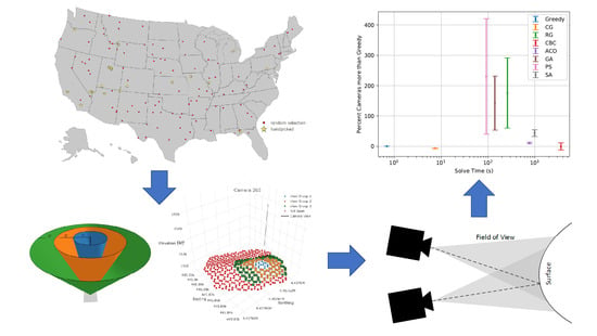
The eight selected algorithms–greedy, RG, CG, CBC, PS, SA, GA, and ACO–appear throughout literature on the SCP, but which algorithm produces optimal view planning for UAVs has not been determined to the authors’ knowledge; the following tests and statistics determine that the CG is the optimal algorithm for the SCP as applied to UAV SfM (in terms that balance solve time and number of cameras required). To analyze each algorithm, two types of sites across the continental United States are evaluated and compared to each other (see Figure 3 and the following list).

• 100 random locations using NumPy’s random number generator with a circle of random radius (50 to 150 m) followed by a perturbation/scaling of the perimeter away from the center (to randomize size, shape, and location before applying the SCP).
• 20 selected sites of interest (selected by the author) including but not limited to include man-made structures, historical sites, and industrial sites (e.g., Tibble Fork Dam, Gettysburg Memorial, Kennecott Copper Mine, Angel’s Landing in Zion National Park, a golf course, the Grand Canyon, and the flat terrain of the Four Corners).

Randomized site locations are chosen to add validity to the statistical analysis as well as normalize the type of terrain with concern to each chosen algorithm. Handpicked sites are chosen because random sites are not guaranteed to process all types of terrain and objects of interest to UAV photogrammetry. Man-made infrastructure, industrial sites, historical monuments, landmarks, and recreational areas are all included in the handpicked sites because such locations and objects are of most interest to reproduce with SfM. Agreement between randomized and handpicked site results would imply that each algorithm performs irrespective of terrain while disagreement between results would emphasize that specific algorithms may perform differently for different terrain types. The Rock Canyon collection dike was chosen for physical flights due to ease of accessibility, permission to fly UAVs in the given airspace, and the variety of terrain and objects of interest at the selected site.

Surface area, change in elevation, and number of data points vary with each site along with steepness and roughness. Steepness is quantified as the average of the absolute value of the first derivative of position (displacement); roughness is quantified as the average of the absolute value of the Hessian (second derivative of position). Three sites are characterized visually in Figure 4 and numerically in

Table 1. Site characterization for three of the 20 selected sites. Elevation plots are included in Figure 4.

Site	Cameras	Points	Area (m${}^2$)	Δ Elevation (m)	Steepness	Roughness (m${}^{-1}$)
Golf Course	653	1956	6628	9.6	0.045	0.003
Grand Canyon	11,371	33,936	503,296	519.4	0.674	0.018
Copper Mine	12,636	37,867	34,798	303.5	0.572	0.079

.

5. Results

5.1. Results for Randomized Sites

Figure 5 marks average solve time and number of needed cameras for the randomly selected sites relative to the greedy algorithm. This was normalization was done by dividing the number of cameras each site required by the number of cameras the greedy algorithm required and calculating a $95\%$ confidence interval based on distributions observed. Camera count is normalized relative to the greedy algorithm due to the fast and simple nature of the base greedy algorithm.

Algorithms that used heuristics, rather than random numbers, to select cameras were generally more efficient. Although PS, SA, and GA, which use random numbers, show superior performance compared to heuristics such as the greedy algorithm in the literature, those studies required few cameras and addressed smaller areas [35,36,38,43,44,45]. Viz, 50 cameras signifies $2^{50}$ or $1.1\times {10}^{15}$ different camera combinations and for 100 cameras becomes $1.2\times {10}^{30}$. The sites in this study range from 265 to 9988 cameras with a median of 2637 cameras and a mean of 3155 cameras. The large camera counts render exploration of the entire search space infeasible when conducted randomly as opposed to a heuristic. Random selection could select a more optimal solution, but given the scale of the search space, the chance of finding an optimal randomly selected set is lower than heuristically selecting a superior data set.

Introducing a heuristic to the PS, SA, or GA methods to replace the random number generator could explore more of the search space. Such adaptations could follow the ACO method’s adoption of a heuristic. Longer run-time or increased iterations increase random variation and would produce additional optima. However, such adaptations to PS, SA, and GA are beyond the scope of this paper (note that while gains may occur, the added solve time could render more complete solutions infeasible).

For number of cameras, the metrics of size of the area compared to number of required cameras provides the essential quantitative analysis (see Figure 6). In accordance with Figure 5, RG, GA, and PS methods perform significantly worse than the base greedy algorithm; however, for CBC and ACO, no clear statistical conclusion follows because although the $95\%$ confidence intervals do not overlap for the randomized sites, CBC and ACO’s $95\%$ confidence intervals do overlap in the upcoming segment that addresses the handpicked site’s results (see also Figure 7). CG performs optimally in both cases.

Besides the direct relationship between size and number of cameras, Figure 6 compares number of cameras to inverse point cloud densities with a fixed intercept of zero to reduce degrees of freedom.

The lowest slope shown in Figure 6 demonstrates that the CG produces models that use fewer cameras and higher resolution (here referring to number of novel points viewed per camera) than the other methods. Although each model achieves similar camera coverage, this does not indicate similar resolution or point cloud densities among camera selection methods.

It should be noted that CBC (the extension of the BIP) performs poorer than expected. This is attributed to solve time limitations, and if solve time were not a constraint, it would likely find the optimal solution.

5.2. Results for Selected Sites

Results for handpicked sites generally follow the results for randomly selected sites. The Pareto Front-esque approach for handpicked sites is similar to the random Pareto Front-esque approach except for a few notable exceptions (see Figure 7). The $95\%$ confidence interval for percentage more cameras for RG, GA, and PS more than doubles. SA and CBC solve slower for the handpicked sites than the random sites (this is attributed to the 1 h permitted solve time instead of the 15 min solve time limit for each random site).

Cameras needed and the model area also differ from added variability of set UAV distance from the ground. The random sites use a set height while the handpicked sites adjust according to the size of site and the required set coverage detail. Distance from the ground clearly impacts the needed number of cameras for a site and this difference is expected.

Figure 8 relates the inverse point cloud density to the number of cameras needed. Despite handpicked site flight variation of flight height, each linear fit has less variation than the random sites. This suggests that man-made structures or locations with distinct features have more predictable relationships between selected cameras and point cloud density.

Again, the CG produces the smallest slope out of all the algorithmic methods. CG delivers higher resolutions per camera in models for comparable areas (for smooth, complex, random, and selected terrains), and the assumption of equal coverage implying equal accuracy appears to be imperfect like the randomized sites’ results.

5.3. Reconciliation of Randomized and Selected Data

Both randomized and handpicked selected data indicate CG as the optimal algorithm for the SCP as applied to UAV photogrammetry and SfM. The CG requires fewer cameras but only an order of magnitude larger solve time than the base greedy algorithm. The traditional greedy algorithm, CG, RG, BIP (in the form of CBC’s COIN-OR solver), swarm intelligence (PS and ACO) and other methods (GA and SA) each explore the same search spaces and data sets to a pre-set coverage parameter of “seeing” $95\%$ of the search space. This study assumes that the coverage metric accurately evaluates each method for every selected site and relies on number of cameras to reach the desired coverage metric (assuming equal coverage also implies similar accuracy). Future work could include other metrics of coverage, analysis to determine how much coverage and accuracy correlate, more detailed model generation, and checking each method with specific sites of interest for optimality to specific site types (e.g., industrial versus civil infrastructure).

6. Grid Independence of CG Parameters

As demonstrated by Pareto Front principles and inverse point cloud density evaluations of the various algorithms, only the CG produces comparable results to the greedy algorithm with fewer chosen cameras without an inordinate time cost. CG follows greedy heuristics but includes $\alpha$ and $\beta$ inputs. As described by Cerrone et al. [28], the $\alpha$ parameter is an integer representing the number of complete revolutions around the subset of data, and the $\beta$ parameter represents a percentage of how much of the whole data-set that is explored with each revolution.

Solve time and number of cameras compete as objectives in a grid independence study, so a grid independence study of the CG parameters explores the required resolution of parameter input. There are many papers that mention the importance of resolution [11,46,47,48,49,50], this suggests how additional numerical analyses could improve algorithms and UAV SfM quality. Breaking up the problem into different scales shows promise in Liu et al. [38].

The calculus-based approach analyzing differential portions or nodes or points of interest and solving them separately (or simultaneously) comes to the forefront since principles used in numerical solutions to partial differential equations (PDEs) relate to UAV SfM algorithmic parameter selection. Heuristics and GAs find reasonable solutions to UAV SfM and take into account (or successfully and accurately ignore) many variables to reach those solutions. PDEs consider multiple differential variables changing simultaneously—most commonly in space and time—so due to similarities in complexities and variables from algorithms and PDEs, it stands to reason that numerical solutions could be obtained similarly. One example drawn from a PDE in computational fluid dynamics points out how grid independence studies are often overlooked despite clear potential to contribute to understanding complex systems [51].

The grid independence study builds on the precedent of prior sensitivity studies for SfM. In Al-Betar et al. [22], the Grey Wolf Optimizer, including a greedy variation combined with genetic concepts such as natural selection, undergoes a sensitivity analysis. Ludington et al. [52] takes georeferenced SfM and uses bundle adjustment to model uncertainty in SfM. Also of particular note, Jung et al. [24] uses a stochastic greedy algorithm for optimal sensor (non-UAV) placement.

Similar to how a generic PDE may be analyzed by a grid of spatial (x) and temporal (t) values, the $\alpha$ and $\beta$ parameters take the place of x and t while the analog z-axis of the 3D reconstructed surface describes either the number of photos or the time to optimize the UAV SfM mission. A refined discretization of the parameters displays the best values when using CG for UAV SfM ($n=1$), an intermediate discretization reveals that the spacing of the chosen discretization is sufficient to have meaningful results ($n=2$), and a broad discretization shows that too wide of a discretization yields unusable results ($n=4$).

Each competing objective respectively becomes the z-axis with $\alpha$ as the x-axis and $\beta$ as the y-axis (see Figure 9). CG solve time increases as either $\alpha$ and/or $\beta$ increase, but as previously shown in Section 5: Results in addressing the statistical comparison of the eight algorithms for the SCP, is only an order of magnitude longer to solve than the base greedy algorithm. The number of cameras chosen by the CG are more sensitive to the input parameters, so

Table 2. Table exploring number of camera benefits for optimized CG parameters in 20 sub-cases.

Greedy	CG	Difference	SD	% SD Fewer
25	24	1	1.87	0.53
33	33	0	1.84	0
43	39	4	3.19	1.25
36	34	2	2.31	0.86
70	65	5	5.27	0.95
27	25	2	1.94	1.03
27	24	3	2.18	1.38
67	62	5	4.68	1.07
46	42	4	3.37	1.19
40	37	3	2.80	1.07
39	35	4	2.85	1.40
75	69	6	5.15	1.16
36	34	2	2.55	0.78
26	25	1	1.59	0.63
79	74	5	5.13	0.97
40	38	2	2.68	0.75
70	63	7	5.29	1.32
37	35	2	2.33	0.86
43	39	4	3.37	1.19
33	31	2	2.27	0.88

(giving the number of cameras used for each sub-case for each algorithm, the difference, and the standard deviation of the camera spread) and

Table 3. Paired two sample for means t-test of Greedy to CG required number of cameras for 20 sub-cases.

t	t Critical	P
7.85	1.73	$1.12\times {10}^{-7}$

explore how much statistical improvement comes from each of 20 sub-cases of the Rock Canyon collection dike (see Section 7: Physical Tet Flights) and yields $3.2$ fewer cameras per model than the traditional greedy algorithm or $96\%$ of one standard deviation (SD) CG parameters. Table 3 is calculated from a one tailed paired two sample for means t-test by comparing the first two columns of Table 2, and the t value is $7.85$, t critical is $1.73$, and the p value is $1.12\times {10}^{-7}$ giving $0.0000112\%$. t is a measure of the variance between the two sets, t critical is the t value that, once passed, indicates statistical significance, and P is a representative probability also used to determine statistical significance. Using a traditional $5\%$p value level of significance, these results are statistically significant and indicate that the greater camera efficiency through CG is not due to chance. Viz, the CG algorithm obtaining fewer cameras in the 20 sub-cases is not likely due to random chance from a base greedy heuristic.

Figure 9 explores the search space of $\alpha$ and $\beta$ for discretizations of $n=1$, $n=2$, and $n=4$ (each of the 120 graphs produces similar results). In other words, $n=1$ signifies the smallest grid squares of $\alpha$ stepping by values of 1 from 0 to 12 and $\beta$ stepping by values of $0.1$ from 0 to $1.2$ (the $beta$-axis is left a factor of 10 too large as 0–12 to mitigate visual distortion and assist visualization the effects of the parameters), $n=2$ are grid squares that are twice as large, and $n=4$ doubles again such that grid squares increase to twice the discretization of $n=2$. Figure 10 and Figure 11 refer to the same study figures on a smaller scale.

The computationally intensive $n=1$ grid squares yield that the number of required cameras for similar coverage minimize at $\alpha =8\pm 1$ and $\beta =0.5\pm 0.3$. The $n=2$ discretization similarly obtains $\alpha =8\pm 1$ and $\beta =0.5\pm 0.3$. However, the $n=4$ grid deviates with $\alpha =6\pm 3$ and $\beta$ losing a defined resolution. The grid independence analysis reveals that the optimal $\alpha$ input is approximately 8 with $\beta$ varying from $0.2$ to $0.8$, and the search space for the parameters could be reasonably adjusted in increments of 2 for $\alpha$ and $0.2$ for $\beta$ to observe differing results.

7. Physical Test Flights

Physical verification of simulation results is an essential step for continued application of research results and occurs periodically in the literature for photogrammetry and SfM [45,53,54,55,56,57,58]. The algorithm set is tested at the Rock Canyon collection dike in Provo, UT, USA. The camera sets chosen for each test are tested for uniqueness (in terms of percentage comparisons based on location/angle metadata and qualitative visual comparisons) to further validate that CG is the most optimal algorithm for the SCP with UAV photogrammetry.

Rock Canyon Collection Dike Algorithm Test Set

The data and analysis of the algorithms at the Rock Canyon collection dike follow the same structure as work by Martin et al. and note “holes” in the created models [10,11]. This extends the previous work which noted “holes” in simulated models but not physical flights.

The Rock Canyon collection dike, though small, contains objects of interest to photogrammetry (e.g., dams, levees, valves). The path for each flight uses a Christofides algorithm to solve the TSP. A DJI Phantom 4 carried out the UAV missions on the same day in a 3 h window (see specifications in

Table 4. Camera specifications for the DJI Phantom 4’s camera.

Sensor	1/2.3″ CMOS
Field of View	94
Image Size (Pixels)	4000 × 3000
Horizontal Viewing Angle	75.2${}^{\circ }$
Vertical Viewing Angle	56.4${}^{\circ }$

) and was flown autonomously with an in-house Android App using DJI’s APK.

Table 5. Summary of algorithm results at the Rock Canyon collection dike.

Method	Cameras	Solve Time (s)	Flight Time (min)
Greedy	49	0.017	9
CG	45	0.094	8
RG	92	1.994	16
CBC	42	3.603	8
ACO	50	36.95	9
GA	61	40.49	10
PS	84	4.471	17
SA	63	10.64	12

summarizes the solve time, the required number of cameras, and approximate flight time for the Rock Canyon collection dike for each algorithm. CG delivers the second lowest camera count (3 cameras above CBC and 4 cameras fewer than base greedy heuristics), the second lowest solve time (behind base greedy), and ties the quickest flight time (same as CBC). CBC delivered the fewest cameras and the quickest flight time, but is sub-optimal because the solve time is 3 orders of magnitude longer than the CG. The CBC algorithms is a worst-case scenario for computation time as it does not leverage heuristics to approximate the solution. These results match the simulations of the algorithms and expected results as discussed previously.

Coverage and uniqueness are evaluated through chosen camera overlap between algorithms. Each algorithm produces a model from a subset of a camera set of 512 potential camera locations for the Rock Canyon collection dike and Equation (13). A route of future research could be a more comprehensive comparison between algorithms from individual flights and applying those same algorithms to an existing data-set of photos to be selected based on photo metadata in terms of shared cameras between algorithms. The method of photo-set metadata to form a histogram matrix of possible viewpoints ensures that the shared cameras are exactly that, shared cameras.

Table 6. Percent common cameras between algorithms following the method shown in Equation (13) where the row represents the reference entity.

	Greedy	CG	RG	CBC	ACO	GA	PS	SA
Greedy	100%	43%	22%	14%	16%	12%	16%	22%
CG	47%	100%	24%	49%	29%	16%	20%	27%
RG	12%	12%	100%	12%	14%	17%	18%	17%
CBC	17%	52%	26%	100%	29%	26%	26%	21%
ACO	16%	26%	26%	24%	100%	14%	22%	16%
GA	10%	11%	26%	18%	11%	100%	20%	13%
PS	10%	11%	20%	13%	13%	14%	100%	14%
SA	17%	19%	25%	14%	13%	13%	19%	100%

gives the percent of commonly chosen cameras between each algorithm. The percentages are not perfectly symmetrical about the comparison of the algorithms with themselves ($100\%$ values in the table) because each algorithm produces differing numbers of cameras that skew percentages depending on which algorithm is the reference algorithm.

As expected, algorithms based on similar heuristics shared common coverage selection, such as the base greedy and CG. However, the highest overlap was the CG and CBC at $52\%$, but the base greedy only overlapped $17\%$ with the CBC. As the CBC solution is the most exhaustive, devoid of heuristic shortcuts, the ratio of common cameras between it and CG lends credibility to the heuristic selection process in CG. As shown in Table 5, the CBC and CG reach the lowest number of cameras, while the CG requires orders of magnitude less time.

Equation (13) demonstrates the method for calculating the common cameras with $n_{common}$ representing mutually common cameras and $n_{reference}$ representing the number of reference cameras. The percent common cameras quantitatively shows that the SCP shares exact camera locations compared to itself but not with the other seven algorithms, so the camera views from each algorithm seem to be more unique than not in terms of geographically chosen viewpoints.

$${\%}_{common}=n_{common}/n_{reference}$$

(13)

However, the null hypothesis, assuming random cameras sets cannot be rejected per Equation (14) and

Table 7. The probability of randomly drawing at least as many in common between two camera sets.

	Greedy	CG	RG	CBC	ACO	GA	PS	SA
Greedy	0%	0%	29%	11%	11%	58%	62%	3%
CG	0%	0%	20%	0%	0%	32%	35%	1%
RG	29%	20%	0%	14%	11%	8%	39%	10%
CBC	11%	0%	14%	0%	0%	1%	8%	7%
ACO	11%	0%	11%	0%	0%	43%	21%	30%
GA	58%	32%	8%	1%	43%	0%	33%	53%
PS	62%	35%	39%	8%	21%	33%	0%	38%
SA	3%	1%	10%	7%	30%	53%	38%	0%

.

$$probability\left(A\right|B)=\left[\sum _{i=n_{com}}^{n_A}\left(\begin{array}{c}{n}_B\\ i\end{array}\right)\left(\begin{array}{c}{n}_{tot}-n_B\\ n_A-i\end{array}\right)\right]/\left(\begin{array}{c}{n}_{tot}\\ n_A\end{array}\right)$$

(14)

The combinations show the probability that camera set A will have at least $n_{com}$ cameras in common with set B, where $n_A$ and $n_B$ are the number of camera in the camera sets and $n_{tot}$ is the total number of cameras that the subsets come from.

Better performing algorithms boast lower probabilities of randomly selecting common cameras, but poorer performing algorithms produce higher probabilities of randomly selecting common cameras.

Observe the full and expanded CDF for each algorithm in Figure 12. The final models are similar to one another with CDF variations of less than $0.02$ for a 4 cm cutoff. Thus, the selected coverage metric to determine if each cameras set gives the desired coverage are all within $2\%$ of one another.

Additionally, the camera overlap of selected methods is shown in Figure 13 as generated by Agisoft. Although only three cameras overlapping make a point visible upon model generation, additional camera overlap adds clarity and resolution. The images demonstrate the qualitatively unique camera locations of each method and that each method garners sufficient coverage of the key area of interest at the Rock Canyon collection dike with overlap of approximately nine or more cameras. Cooler colors indicate greater overlap and warmer colors indicate fewer cameras that overlap in the final models. Each of the four camera overlap images covers the same general area but visibly overlap differently. Each black dot shows the location of a camera projected to the ground, and the difference of cameras is particularly visible with a close look at the PS overlapping compared to the other three. The visible difference qualitatively demonstrates that the cameras from each algorithm are unique (at least in aggregate) because what each camera “sees” is not the same even though the terrain and overall coverage theoretically remain equal, and the same pool of photos built the histogram of viewpoints.

In summary, the set of algorithms applied to the Rock Canyon collection dike confirm the simulation results that the optimal UAV photogrammetric SCP algorithm, as constrained by time and number of cameras, is the CG. The CG requires less time and fewer cameras to produce similar coverage (within $2\%$) of each other method for the case study with a unique set of camera locations–none of the solutions sets are exactly the same. Future work could include subdividing buckets or minimizing distances between cameras within the algorithms.

8. Discussion

The current study is an initial study in how to optimize both computational resources and flight time to create sufficient coverage for a SfM model. The authors are aware of progress within the realm of flight planning and next-best-view planning; however, the computational strain of large amounts of photographs is significant. By optimizing number of cameras and constraining coverage, models can be created with less computational and flight time. Additional work may be done to quantify the identified algorithms’ computational time with a more generalized computational complexity measure rather than run-time on an example computer.

The current work selects areas using distorted circles at various sites within the continental United States. Since the sites were distributed randomly, the results are likely generalizable to the United States as a whole, but only if the areas are roughly circular as they were in this study. Further research could study the effect of the shape of the area of interest on cameras required for coverage. In addition, publicly available data was used for the a priori basis of the models as well as calculating coverage. This data was available at a resolution of one elevation point per square meter. Further research could observe the effects of more detailed a priori data.

More thorough comparison of the observed algorithms (such as using buckets or adjusting solve time requirements), and comparison with more algorithms would strengthen the data analysis. In addition, different methods of establishing the best viewpoints such as next-best-view models could prove valuable. Many of the algorithms used could be improved through a refined balance of heuristic and random choosing methods. The incorporation of simulation environments such as Terragen and Microsoft AirSim to carry out extensive tests for many theoretical environments would be another aspect to explore. Although this study uses USGS and Google Earth data for modeling, in many cases, there is little-to-no knowledge of the area before flight. Research into iterative or dynamic modeling without using initial data will also become valuable to the discussion of the SCP, photogrammetry, and infrastructure modeling with UAVs.

Finally, flight planning bridges the gap between academic research, theoretical work, and in-field implementation. More robust methods of ensuring no collisions during the flight planning stage would prove invaluable. This proves especially true when little or no a priori knowledge exists, or where the a priori knowledge is incomplete.

9. Conclusions

Optimization of viewpoints for SfM model creation minimizes flight time and required computational resources. The greedy algorithm and similar heuristics are well adapted to select locally optimal solutions without a large computational price. Of the eight algorithms (greedy, RG, CG, CBC, PS, SA, GA, and ACO) studied in the context of SfM, only the CG algorithm improved the number of photos required to model topographic areas in simulation while not causing multiple orders of magnitude increase in computational solve time. These results also prove consistent in both simulation of 100 locations and the field test in Rock Canyon Park in Provo, UT, USA. CG obtains the same or fewer required number of cameras as the base greedy algorithm (averaging a statistically significant $3.2$ fewer cameras) for the same SCP with only one order of magnitude longer solve time. Linear programming for similar results requires at least 3 orders of magnitude longer than the CG to solve. A brief grid independence study identifies the optimal parameters for the CG to be $\alpha =8\pm 1$ and $\beta =0.5\pm 0.3$.