Refining the Joint 3D Processing of Terrestrial and UAV Images Using Quality Measures


1
3D Optical Metrology (3DOM) Unit, Bruno Kessler Foundation (FBK), Via Sommarive, 18, 38123 Trento, Italy
2
Dipartimento di Ingegneria e Scienza dell’Informazione (DISI), Universitá degli Studi di Trento, Via Sommarive, 9, 38123 Trento, Italy
*
Author to whom correspondence should be addressed.
Remote Sens. 2020, 12(18), 2873; https://doi.org/10.3390/rs12182873
Submission received: 6 August 2020
/
Revised: 27 August 2020
/
Accepted: 31 August 2020
/
Published: 4 September 2020
(This article belongs to the Special Issue Latest Developments in 3D Mapping with Unmanned Aerial Vehicles)
Abstract
:The paper presents an efficient photogrammetric workflow to improve the 3D reconstruction of scenes surveyed by integrating terrestrial and Unmanned Aerial Vehicle (UAV) images. In the last years, the integration of this kind of images has shown clear advantages for the complete and detailed 3D representation of large and complex scenarios. Nevertheless, their photogrammetric integration often raises several issues in the image orientation and dense 3D reconstruction processes. Noisy and erroneous 3D reconstructions are the typical result of inaccurate orientation results. In this work, we propose an automatic filtering procedure which works at the sparse point cloud level and takes advantage of photogrammetric quality features. The filtering step removes low-quality 3D tie points before refining the image orientation in a new adjustment and generating the final dense point cloud. Our method generalizes to many datasets, as it employs statistical analyses of quality feature distributions to identify suitable filtering thresholds. Reported results show the effectiveness and reliability of the method verified using both internal and external quality checks, as well as visual qualitative comparisons. We made the filtering tool publicly available on GitHub.
1. Introduction
In the last years, Unmanned Aerial Vehicle (UAV) platforms [1,2,3,4] have become widely used for image or LiDAR (Light Detection and Ranging) data acquisitions and 3D reconstruction purposes in several applications [5,6,7,8,9,10,11]. Such platforms have brought undisputed advantages, in particular when combined with terrestrial images. The increasing number of applications where UAV-based images are combined with terrestrial acquisitions is related to the opportunities to achieve complete and detailed 3D results. Despite the promising results of this image fusion approach, several issues generally arise from the joint processing of such sets of data. Big perspective changes, different image scales and illumination conditions can, in fact, deeply affect the adjustment and orientation outcomes and, consequently, the successive photogrammetric products.
Nowadays, the automation of image-based techniques has simplified the procedures of 3D reconstruction, also allowing non-expert users to digitally reconstruct scenes and objects through photogrammetric/computer vision methods. In automatic processing pipelines, increasingly robust operators and algorithms have reduced the manual effort and the processing time required in the traditional photogrammetric procedures. At the same time, however, these solutions offer less control over the processing steps and the quality of the final products.
The quality of the generated 3D data strongly depends on the characteristics of the employed sensors, on the photogrammetric network design and on the image orientation results. In many close-range and UAV-based applications, non-metric and low-cost cameras are frequently used and combined, while highly automatic algorithms of Structure from Motion (SfM) and Multi-View Stereo (MVS) commonly available in open-source and proprietary software [12,13] support the processing of image datasets. Nevertheless, characteristics of the acquired images (in terms of resolution, exposure, contrast, etc.), as well as block geometry configuration, and features extraction and matching procedures, are unavoidable factors conditioning the quality of the orientation process and the resulting reconstruction products [14].
Camera parameters and sparse point clouds are simultaneously computed using a bundle adjustment procedure based on image features automatically extracted from the set of acquired images. The quality of the image orientation, however, does not depend only on the number of the extracted points, which have a limited effect on the network precision, but rather from their correctness [15]. Wrong matched correspondences can negatively affect the bundle adjustment results and return noisy MVS-dense point clouds.
In multi-scale and multi-sensors acquisitions, which imply a combination of different network configurations, issues in the orientation step and unsatisfactory reconstruction results are even more evident [16]. Therefore, the improvement of the quality of image-based 3D processes is closely linked to a more in-depth analysis and control of the bundle adjustment results.
Paper Aim and Novelty
The work presents a methodology to detect and remove outliers and wrong matches affecting the image orientation results in automated image-based 3D processes. The proposed method allows to obtain more accurate camera parameters and so more dense and accurate dense point clouds by MVS. Quality metrics are firstly derived for the 3D tie points computed within the bundle adjustment step (Section 3.2), then aggregated in order to filter the sparse point cloud (Section 3.3) and derive a new set of tie points. The camera parameters are then re-computed with a new adjustment and the filtered tie points before generating a dense 3D reconstruction.
The work extends the method presented in [16,17] and employs only photogrammetric parameters for the quality analyses, adopting a robust statistical approach for thresholds identification in the filtering step. Although, in fact, the previous approaches based on geometrical parameters returned satisfactory results, the procedure was quite time-consuming and several issues arose working on very sparse data. Therefore, the statistical distribution of the quality parameters is used for the automatic identification of suitable thresholds for removing bad tie points, increasing the applicability and replicability of the procedure. Moreover, a more reliable weighting procedure is introduced for assigning a quality score to each 3D tie point, replacing the testing phase of several weight combinations for each quality parameter [16].
2. State of the Art
In every 3D surveying project, planning an optimal image network configuration, suitable to completely and accurately survey a scene, is the key step for achieving the expected reconstruction results and needs. Nevertheless, in the common 3D surveying practice, no planning is performed, and the quality of the final 3D results is amended by managing and controlling the image processing parameters. The integration of terrestrial and UAV images (often called “data fusion”) for surveying large and complex scenes further enhances this issue. Such images are usually characterized by big perspective changes and different image scales besides frequent illumination variations, especially in diachronic acquisitions. These particular conditions make the matching phase very complex, with a variable number of correspondences detected among heterogeneous image blocks and recurring errors in the identified homologous points.
In the following sections, we will report related works about data fusion (Section 2.1), image network design (Section 2.2) and point cloud filtering (Section 2.3), all aspects related to the presented paper.
2.1. Data Fusion
Sensor and data fusion refer to the process of integrating acquisition sensors, acquired data—commonly at different geometric resolution—and knowledge of the same real-world scene. The fusion is generally performed in order to create a consistent, accurate and useful digital representation of the surveyed scene. The fusion processes are often categorized as low, intermediate or high, depending on the processing stage at which fusion takes place [18,19,20]. Low-level data fusion combines several sources of raw data to produce new raw data. The expectation is that fused data are more informative and resolute than the original inputs. Medium level merges features coming from different raw data inputs, whereas high-level fusion is related to statistic and fuzzy logic methods. The fusion is normally performed to overcome some weaknesses of single techniques, e.g., lack of texture, gaps due to occlusions, non-collaborative material/surfaces, etc. For fusing different data, it is indispensable to have a set of common references in a similar reference system clearly identified at each dataset. These common references can be either one-, two- or three-dimensional, and can be identified either manually or automatically. Data fusion has been applied for many years in various fields, such as cultural heritage documentation—especially when large or complex scenarios are considered and surveyed [21,22,23], remote sensing [24,25,26], spatial data infrastructures [27], smart cities [28], etc. What is so far missing is a smart way of integrating data and sensors; indeed, none of the published methods so far fuse data based on quality metrics.
2.2. Image Network Configurations
The impressive technological advancements in terms of automated algorithms for image orientation (SfM) have led users to two facts: (i) being able to generate nice textured 3D results with minimum manual efforts and (ii) acquire many images, very often more than those strictly necessary, with an unfavourable geometry and not in the appropriate positions. However, the effectiveness of automated processing algorithms in identifying and matching correspondent features in overlapping images is often not sufficient for guaranteeing the achievement of the required accuracy and completeness of the 3D reconstruction. Image network design and its quality have been deeply investigated [29,30,31,32,33,34]. The relevance of suitable base-to-height ratios and camera parameters [15,29,35], advantages of bigger intersecting rays, as well as higher image redundancy [36,37], have been analyzed to identify the achievable accuracy with some standard and straightforward image network configurations. The quantitative and rough estimation of the expected quality for a designed camera network has been proposed in [29]:
where the precision in direction (camera-to-object) in the case of orthogonal acquisitions is determined as a function of the distance to the object, the baseline (i.e., distance among two cameras), the camera focal length and the precision of the image measurements (which depends on the accuracy of the feature extraction and matching). The role of the baseline is changed in the last years as, contrary to theory, short baselines are required by automatic image matching procedures, as big perspective changes can cause a decrease in the object precisions.
In the very common case of convergent images, the proposed Equation (1) can be generalized for all object coordinates as:
where k is the number of images for each camera position (generally 1) and is a design factor, indicating the quality of the imaging network and depending on the intersection angle between homologous rays (with optimal network 0.5 < < 1.2). The homogeneity of the precision values is reached when intersection angles are near to 90°.
The proposed formulas for estimating and analyzing the quality of the camera network are, however, only applicable when a uniform and regular acquisition geometry is respected, a single sensor is used for the image capture and the environment can be controlled. When data are multi-sensor and multi-scale and scenes are quite complex, further investigations are needed, involving, e.g., metrics produced by the bundle adjustment process [12].
In the last years, quality assessments for different block configurations design have been partially explored for close-range terrestrial and UAV-based acquisitions [38]. Methodologies for checking the quality of the obtained results, deformation analyses and some recommendations with typical photogrammetric networks, especially employed in the cultural heritage field, have been presented in [14,39]. Results of different imaging geometries for large-scale acquisitions are compared in the close-range terrestrial scenario and when UAV and terrestrial images are processed. Reference [40] proposed a broad quality assessment in different acquisition scenarios, comparing different network configurations and processing conditions (e.g., weak image blocks, effects of self-calibrations, the influence of Ground Control Points (GCPs) and their distribution, number of extracted tie points and consequences of some image acquisition settings). In [41], the effects on the object points precision with complex network configurations and significant image-scale variation are deepened, analyzing the quality of the bundle adjustment results with irregularly distributed camera stations.
2.3. Point Cloud Filtering
Sensors limitations, weak acquisition geometries and issues in the processing steps can return noisy and incomplete 3D reconstructions. Noise and outliers are random errors in the measured data and points which behave differently from a set of normal data, respectively. These are common phenomena in both range-based and image-based data, and they can be solved or mitigated through a filtering step.
The solutions proposed in the last years can operate at different levels (i.e., sparse or dense point clouds or meshes). However, most of them are focused on specific methods for denoising meshes. Fewer methodologies have been instead implemented for point clouds, despite the obvious advantages of working on a lower data level [19] in terms of reduced computational efforts and improvement of the following reconstruction products. An extensive review of the developed algorithms for filtering point clouds has been proposed by [42].
Depending on the specific nature of 3D point clouds, many approaches are based on statistical methods [43]. These methods assume that data follow some statistical models for classifying points as outliers, defining probability distribution functions [44] or assigning specific weights in statistical denoising frameworks [45,46]. Global or local solutions proposed for outlier detection and removal are mainly based on a balance between the cleaning demand and the preservation of the features or/and shape. Most of the proposed filtering and smoothing methods analyze some local or global geometric properties computed on the point clouds [17,47]. Projection-based filtering techniques use several projection strategies on estimated local surfaces for identifying outliers. Many of these approaches are based on regression methods, such as the Moving Least Square (MLS) [48].
Other, more specific procedures have been developed for denoising image-based point clouds and improving the entire photogrammetric workflow. Following initial works based on efficient solutions for the extraction of reliable and accurate tie points [49,50,51], more recent studies focus on tie points, filtering for improving the orientation step. In the context of UAV-based datasets, [52] presented an outlier detection method based on the statistical distribution of the reprojection error, proposing a noise reduction procedure that considers the intersection angles among homologous rays. In [53,54] new strategies to assign quality measures to the extracted tie points were proposed in order to refine the camera parameters through a filtering step based on the acceptable reprojection error and the homogenous distribution of tie points. These methods offer a deeper knowledge of quality issues which could affect the following products, working at a lower level (i.e., on the first reconstruction results). In [55], input images and depth map information are used to remove pixels geometrically or photometrically inconsistent with the input coloured surface.
Finally, a more recent group of filtering approaches is based on the application of deep learning algorithms to 3D data [56].
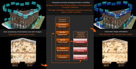
3. Proposed Methodology
This section presents the pipeline implemented to improve the orientation and 3D reconstruction results when terrestrial and UAV-based imageries are jointly processed. The procedure (Figure 1) features an initial filtering step (Section 3.3) based on some quality parameters (Section 3.2) of the 3D tie points computed within the bundle adjustment. After such filtering, the bundle is again repeated using only high-quality tie points in order to compute more precise camera poses. The filtering pipeline, developed in Python, is available at https://github.com/3DOM-FBK/Geometry.
3.1. Work Premise and Motivation: Challenging Image Network Configurations
Before developing the filtering methodology (Section 3.3), some tests were conducted to recap the effects of different image networks (terrestrial with convergent images, terrestrial with almost parallel views, UAV or combined) on the photogrammetric processing and on the achievable accuracies (hereafter measured with the a-posteriori standard deviation σ computed within the bundle adjustment process).
Figure 2 and Figure 3 show the considered image network and error distributions, respectively. The errors are also more accurately summarized in Table 1.
The first three cases are consistent with the expected results. Average σ values are generally higher in the camera depth directions. In the convergent geometry (network 1a), average σ values are higher in the x-y plane; with parallel views images (network 1b), precision is worse along the camera depth direction (y-axis); with UAV images (network 1c), the precision is worse in the y-z plane. Furthermore, reconstructed 3D tie points show higher σ values when the sensor-to-object distance increases.
From the joint processing of terrestrial and UAV images (network 1d), a more homogeneous error distribution in the three directions can be noticed, as well a general worsening of most of the statistical values. This highlights that the combination of different scale and sensor data, which returns hybrid and complex imagery geometries, define challenging processing scenarios where outliers and wrong computed matches frequently and heavily affect the quality of the image orientation and 3D reconstruction. The effectiveness of the implemented filtering procedure is tested on these challenging data, and results are presented and discussed in Section 4.
3.2. Quality Parameters of 3D Tie Points
The quality of the camera orientation process can be derived from external and internal consistency checks [31]. While checking the results with external data provides a measure of possible block deformations, internal statistics are reliable indicators of the quality of the features extraction and matching steps, and, indirectly, of the image block strength.
In this work, some inner quality parameters of each 3D tie point [12,16,57] are computed with an in-house tool and used to remove bad-quality tie points. The considered parameters express the quality of the image network geometry, the correctness of the matching and adjustment step, as well as the reliability and precision of the reconstructed 3D points. We consider the following quality parameters of the sparse point cloud derived within the bundle adjustment procedure (Figure 4):
- (a)
- Re-projection error (or image coordinates residuals): it represents, in image space, the Euclidean distance between the measured point position and the back-projected position of the calculated 3D point. Even though low re-projection error values can suggest a high quality of the computed 3D point, this feature is not very significant when the point has been measured in few images.
- (b)
- Multiplicity (or image redundancy): this value indicates the number of images contributing to the 3D point calculation, i.e., the number of images where the point has been measured. Therefore, the multiplicity value refers to the excess of image observations with respect to the number of unknown 3D object coordinates, estimated within the adjustment step. High multiplicity values suggest greater reliability and precision of the computed 3D tie points, considering that multiple intersecting rays contribute to the point position check.
- (c)
- Maximum intersection angle: it refers to the maximum angle between intersecting rays contributing to the creation of a 3D point. Small intersection angles can negatively affect the adjustment procedure and reduce its reliability.
- (d)
- A-posteriori standard deviation of object coordinates (σ): from the covariance matrix of the least squares bundle adjustment, the standard deviations of all unknown parameters can be extracted. High standard deviation values can highlight 3D points with unsuitable object coordinates precision and problematic areas within the image network.
3.3. Filtering Technique
Once each 3D tie point is enriched with its quality parameters (Section 3.2), an aggregated quality score is computed as a linear aggregation of the different parameters (Section 3.3.2). The aggregated quality score of each 3D tie point is used as an indicator of the quality of the reconstructed point within the adjustment procedure. This quality measure is employed in the automatic filtering approach to discard low-quality points (Section 3.3.3) before running a new bundle adjustment to refine the orientation results.
3.3.1. Single-Parameter Filtering: Tests and Issues
Many filtering methods employ a single quality parameter to discard bad points. To highlight that quality features are correlated and should be concurrently considered, a dataset of 133 terrestrial and 87 UAV images (Section 4.1.1) is processed in order to derive camera parameters and a sparse 3D point cloud. Quality parameters (re-projection error, multiplicity, intersection angle and a-posteriori standard deviation) are then individually used to filter bad 3D points, a new bundle adjustment is performed, and new quality parameters are computed. Table 2 shows the variations of the single quality parameters when only one is used to filter the sparse point cloud derived from the bundle adjustment. The variations of the median values are not consistent, e.g.: filtering tie points considering only their multiplicity leads to a higher multiplicity but a worse median re-projection error; filtering using only the re-projection error decreases the median intersection angles, etc. Such results confirm the limits of a single-feature filtering approach and the need of adopting a filtering method based on combined and aggregated parameters.
3.3.2. Normalization and Linear Aggregation
A data normalization process is mandatory for assigning equal weight to each quality parameter. Through several statistical approaches of normalization, differently measured and computed values can be adjusted and scaled in the same range [0, 1] [58].
In the past research [16], a min–max features scaling method was tested, with a simple linear transformation allowing independent variables to be rescaled in the same range based only on the minimum and maximum value.
In the current work, we explore the advantages of adopting a logistic function for representing and scaling the data, thus reducing the outliers’ effect. The employed logistic function is represented by a sigmoid curve and an inflection point (sigmoid midpoint). Outliers are penalized by the characteristic trend of this curve, which exponentially grows but slows down its growth moving close to the boundaries. In the general formulation, the function is expressed as Equation (3):
where:
- is the maximum value of the curve;
- is the Euler’s number;
- is the x value of the sigmoid’s midpoint;
- is the steepness of the curve.
The two main variable and adjustable parameters of this function are and (vertical and horizontal scaling parameters), which define how the curve is stretched or compressed to better fit the data. Following [59], we adopted a modified logistic function which proved to be efficient with comparable normalization issues:
where is the value to normalize, the mean and the standard deviation of the data.
The normalized quality parameters values are then linearly combined with the proposed aggregation method Equation (5):
- is the overall aggregated quality score computed with the normalized quality parameters for each 3D tie point;
- is the normalized value of the re-projection error;
- is the normalized value of the multiplicity;
- is the normalized maximum angle of intersection;
- is the normalized value of the a-posteriori standard deviation;
- is a weight computed for each 3D tie point as in Equation (6):
3.3.3. Filtering Threshold Identification—The Statistical Approach
Once an aggregated quality score is assigned to each 3D tie point (Equation (5)), the identification of suitable thresholds for keeping only good-quality 3D points proved to be a very challenging task. Limits for filtering points, based on the respective aggregated score, are computed as the sum of single feature thresholds. The choice of using optimal values for each feature threshold, as presented in [16], hardly generalizes to every type of dataset and/or image block. Aiming at generalizing the filtering methodology, i.e., at automatically identifying suitable thresholds for each dataset, the statistical distribution of each quality feature is here considered. The analysis of values distribution for each quality parameter is particularly helpful for outlier identification, as well as for highlighting wrongly computed tie points, resulting from a weak image block geometry or issues in the matching and adjustment steps.
From the theory of errors, the general assumption is that random errors in a set of data have a normal distribution [31]. In the probability density function of a Gaussian distribution, the probability that the random error of variables lies in certain limits is defined as a symmetrical factor of the standard deviation. A common approach for the outlier removal is based on filtering data exceeding the “3σ rule”. Therefore, mean values, plus or minus three standard deviations, are employed as thresholds for removing outliers, considering that 99.87% of data are distributed within this range [60]. Other authors have suggested less conservative approaches and a reduction of the considered standard deviations around the mean [61,62].
Nevertheless, in laser scanning and photogrammetric data, a deviation from a normal trend is frequently observed, especially due to outliers. The normality assessment can be supported by statistical analyses and parameters, such as the Q-Q plot (quantile-quantile) or the Skewness and Kurtosis values [62]. More robust approaches with respect to the 3σ rule method must be employed with large datasets heavily affected by outliers, or when Skewness and Kurtosis values prove a non-normal behaviour of the distribution of the errors [63,64]. In these cases, sample quantiles of distribution are usually used. The quantile of a distribution is the inverse of its cumulative distribution function. The 50% quantile is the median of the distribution and it is a robust quality measure, less sensitive to outliers, that performs better with skew distributions.
Another robust estimator is the σ, derived from the Median Absolute Deviation (), i.e., the median of the absolute deviations from the median of all data:
where b = 1.4826 is a general assumption of the normality of the data, disregarding non-normal behaviour introduced by outliers. In this work, median and median plus σ values are considered as possible thresholds for each quality parameter, as explained in the next section. Tests and results adopting the median plus 3σ features’ values provide negligible effects on the sparse point cloud filtering.
3.3.4. Thresholds Tests
The robust statistical approaches described in the Section 3.3.3 for the identification of parameter thresholds were tested and the average improvement of quality features compared. In particular, using a dataset of 133 terrestrial and 87 UAV images (Section 4.1.1), the following filtering thresholds were considered:
- (1)
- Median values for each quality parameter, not weighting the aggregation function;
- (2)
- Median values for each quality parameter, weighting the aggregation function;
- (3)
- Median plus σ, not weighting the aggregation function;
- (4)
- Median plus σ, weighting the aggregation function.
Table 3 reports the improvements of the computed quality parameters for the considered threshold approaches.
A more aggressive filtering approach (i.e., case 1 and 2) produced a considerable improvement of the quality parameters. A less aggressive filtering (case 3 and 4) delivers more homogeneous results and removes less 3D points. The encouraging effects of a less conservative method (such as case 2), also confirmed by the other datasets and tests, supported the choice of selecting the median values as feature-threshold. A quite aggressive filtering (such as case 1) involved removing too many tie points, and images could not be oriented.
4. Test and Results
4.1. Experiments and Results
In the following sections, different case studies are presented to demonstrate the effectiveness and replicability of the developed methodology. The implemented and tested filtering procedure follows the subsequent steps (Figure 1):
- (a)
- Perform the joint processing of UAV and terrestrial images in order to compute camera parameters, sparse and dense point clouds;
- (b)
- Compute quality parameters for each 3D tie point of the sparse point cloud (Section 3.2);
- (c)
- Normalize the computed quality values and their aggregation (Section 3.3.2), for assigning a quality score to each computed 3D tie point;
- (d)
- Analyze the statistical distribution of the computed quality parameters and identify suitable thresholds for each dataset (Section 3.3.3 and Section 3.3.4);
- (e)
- Filter those 3D tie points with an aggregated score higher than the selected threshold and generate a new set of filtered tie points;
- (f)
- Run a new bundle adjustment, refine the camera parameters and generate a new sparse point cloud;
- (g)
- Re-compute quality parameters on the filtered and refined cloud for evaluating the improvement of the inner quality parameters with respect to step (b);
- (h)
- Compute a new dense point cloud;
- (i)
- Employ external checks (e.g., 3D ground truth data) and noise estimation procedures to evaluate improvements of the newly generated dense point cloud with respect to the dense point cloud obtained from step (a).
4.1.1. Modena Cathedral
The dataset of the Modena Cathedral (Italy) is composed of 219 images (Figure 5), with 133 terrestrial images and 87 acquired with a UAV platform. The terrestrial images (average GSD: 2 mm) were acquired with a Nikon D750 (pixel size of 5.98 µm) with an 18 mm (73 images) and 28 mm lens (59 image). The UAV images (average GSD: 8.3 mm) were acquired with a Canon EOS 600D (focal length of 28 mm, pixel size of 4.4 µm).
From the joint orientation of the terrestrial and UAV images, about 405,000 3D tie points were derived in the sparse point cloud. Using the in-house Python tool, the initial quality parameters were extracted for each 3D tie point (Table 4).
Aggregated median values were selected as a threshold in the filtering step (Section 3.3.4). About 280,000 3D tie points, with an aggregated score higher than the selected threshold, were automatically removed. The filtered set of tie points was then used for running a new bundle adjustment and refining the orientation results. Table 5 reports values and average improvements with respect to the original sparse point cloud of the recomputed quality parameters. The normality assessment of the a-posteriori standard deviation values before and after filtering, as well as related Kurtosis and Skewness parameters, are shown in Figure 6.
For the external quality check, a laser scanner point cloud (spatial resolution of 1 mm) was acquired with a Leica HDS7000. A seven parameters Helmert transformation was performed in order to co-register the photogrammetric and ranging point clouds. Then, the photogrammetric dense clouds obtained from the original processing and the one produced after the filtering step were compared with the reference laser scanning data. Using some selected areas (Figure 7), RMSEs (Root Mean Square Errors) of plane fitting procedures (Table 6) and cloud-to-cloud analyses (Table 7) were performed. In both cases, the quality improvements of the dense point cloud derived after the filtering procedure was remarkable.
Finally, a visual evaluation of the quality improvement is shown in Figure 8, where noise reduction and a more detailed reconstruction of the marble surfaces are visible.
4.1.2. Nettuno Temple
The “Nettuno Temple” in the Archaeological Site of Paestum (Italy) [65] was surveyed, combining some 214 UAV images and 680 terrestrial images (Figure 9). For the UAV-based images a Canon EOS 550 D (pixel size 4.4 µm) with a 25 mm lens was employed (average GSD: 3 mm), while the terrestrial images were acquired with a Nikon D3X (pixel size 5.9 µm) and a 14 mm lens average terrestrial GSD 2 cm).
The joint processing of UAV and terrestrial images produced a sparse point cloud with some 640,000 3D tie points. Results of the quality parameters extracted from the derived sparse point cloud are presented in Table 8.
Once a suitable threshold was identified (Section 3.3.4), the automatic filtering procedure returned a new set of 3D tie points of about 187,000 (~71% of the original sparse cloud were removed). Results and improvement of the inner quality parameters for the Nettuno temple dataset after running a new bundle adjustment are shown in Table 9.
In order to further evaluate the improvements of the filtering procedure with respect to external information, RMSEs on 30 total station check points (Table 10) and cloud-to-cloud analyses on five sub-areas (Figure 10 and Table 11) surveyed with laser scanning (spatial resolution 5 mm) were performed. For this case study, the improvement brought by the proposed filtering procedure was very evident.
Finally, some visual comparisons of the dense point clouds produced with a standard procedure (“original”) and the proposed filtering procedure (“filtered”) are provided in Figure 11.
4.1.3. The World War I (WWI) Fortification of Mattarello (Trento, Italy)
One side of the WWI Fortification of Mattarello (Trento, Italy) was surveyed, integrating 68 terrestrial and 14 UAV images (Figure 12). Terrestrial images (average GSD: 2 mm) were acquired with a Nikon D750 (pixel size of 5.98 µm) with a 50 mm lens, while the UAV images (average terrestrial GSD: 1.3 cm) were acquired with a FC6310 camera (focal length of 8.8 mm, pixel size of 2.6 µm).
From the joint processing of UAV and terrestrial images, some 1.2 mil. 3D tie points were computed and their quality parameters extracted, as shown in Table 12.
Adopting the proposed filtering procedure, some 717,000 tie points were removed (~61%). Results of the inner quality parameters variation are shown in the Table 13.
For the external check, a laser scanner point cloud acquired with a Leica HDS7000 was employed (spatial resolution of 1 mm). Results of the cloud-to-cloud distance procedure on five sub-areas (Figure 13) are presented in Table 14. Qualitative and visual analyses and improvements are shown in Figure 14.
4.1.4. The ISPRS/EuroSDR Dortmund Benchmark
The central part of the Dortmund benchmark [66] was considered. It contains the City Hall (Figure 15) seen in 163 terrestrial images (average GSD: 3 mm) acquired with a NEX-7 camera (16 mm lens, 4 µm pixel size) and in 102 UAV images (average GSD: 2 cm) captured with a Canon EOS 600D (20 mm lens, 4.4 µm pixel size).
Statistics computed on the extracted quality parameters of the original sparse point cloud (~315,000 tie points) are shown in Table 15, while results on the filtered tie points set (~70,000 points) are given in Table 16.
5. Discussion
The presented work extends two previous studies [16,17], proposing a new approach for achieving even better improvements in the 3D reconstruction results with a more flexible and time-preserving procedure. Limitations and weaknesses of the precedent methods pushed authors to develop the current work, based only on photogrammetric quality parameters and a robust statistical approach for the filtering step. Statistically defined thresholds instead of strict and idealized values, as in [16], avoid the risk of an excessive filtering of tie points, increasing the feasibility of the procedure. The proposed weighted aggregation function (Section 3.3.2), based on the tie point multiplicity, allows for overcoming the time-consuming testing of several weight combinations for each quality parameter. Compared with the geometrical method presented in [16], the current filtering procedure is based only on photogrammetric parameters and proved to be more efficient. In the geometrical approaches, the suitable identification of optimal radii for the feature extraction strongly conditions the filtering results, and it proved to be a very challenging task working on sparse data. With respect to similar filtering approaches based on the quality analyses of computed 3D tie points [52,53], our method considers various and combined photogrammetric parameters for defining the quality of the reconstructed 3D points. The novelty and importance of their aggregation, as presented in Section 3.3.1, is related to the insufficient improvements of the single-features filtering approach.
Quantitative and qualitative results and analyses of the developed method have been extensively reported with four case studies. For verifying the robustness and effectiveness of the procedure, the presented datasets differ for the number of processed images, employed sensors and camera network geometries. A summary of the main results and average improvements of the reconstructions adopting the proposed filtering workflow is presented in Table 19.
Although results clearly show the relevant benefits of adopting the presented method for refining the image orientation, some issues and limitations of the procedure have to be highlighted:
- (a)
- the filtering method does not fully consider the tie point distribution in image space. Too aggressive filtering could prevent the orientation of some images during the orientation refinement. This issue is partially solved by adopting more relaxed thresholds, as presented in Section 3.3.4, and weighting the aggregation function.
- (b)
- the presented method has not been yet verified in the case of multi-temporal datasets.
- (c)
- the computation of the quality features and the filtering procedure are performed with an in-house developed tool (https://github.com/3DOM-FBK/Geometry) which has been so far tested only in combination with the exported outputs from the commercial software Agisoft Metashape [67]. Some issues about file format compatibility could arise while testing our filtering tool in combination with other open or commercial software.
6. Conclusions and Future Works
This paper presented an enriched photogrammetric workflow for improving 3D reconstruction results when terrestrial and UAV images are jointly processed. In the last years, the unquestionable advantages of integrating these different sensor imageries have encouraged their use in several fields, from building to urban scales. Nevertheless, various sensor characteristics and environmental constraints, as well as irregular and unconventional camera network configurations, commonly affect the quality of the image orientation and 3D reconstruction results. This work deals with these processing issues, proposing an extended photogrammetric workflow where a filtering step is performed on the initial image orientation results. In the developed procedure, the initial sparse point cloud is filtered, a new bundle adjustment is performed to refine the camera parameters and, finally, a dense 3D reconstruction is generated. The filtering step is based on the evaluation of quality parameters for each 3D tie point computed within the bundle adjustment. The aggregation of these quality metrics allows removing low-quality tie points before refining the orientation results in a new adjustment. Thresholds for removing low-quality points are based on the statistical distribution of the considered quality parameters. The proposed robust statistical approach extends the feasibility of a previous method [16] to different quality datasets, and it is time-efficient if compared with other geometrical approaches [17].
The effectiveness of the developed procedure was tested on several datasets, all featuring terrestrial and UAV images and different scenarios. Relevant result improvements were proved using internal and external quality checks. The visual and qualitative comparisons of the dense reconstructions, generated with the standard and enriched workflow, show the relevance of the procedure.
Further tests will investigate the effectiveness and robustness of the proposed method with multi-temporal datasets, where complex network geometries and scene changes usually return unsatisfying 3D reconstruction results. In addition to that, the filtering procedure will be extended to consider also the tie point distribution in the image space. This could help to preserve a homogeneous distribution of the tie points in the image and prevent aggressive filtering.
Author Contributions
The article presents a research contribution that involved authors in equal measure. In drafting preparation, F.R. supervised the overall work and reviewed the entire paper, writing the introduction, aim and conclusions of the paper; E.M.F. dealt with the state of the art, methodology, data processing and results. A.T. was mainly involved in the development of the filtering tool, methodology development and paper revision. All authors have read and agreed to the published version of the manuscript.
Funding
This research received no external funding.
Acknowledgments
The authors would like to acknowledge the provision of the datasets by ISPRS and EuroSDR, released in conjunction with the ISPRS scientific initiative 2014 and 2015, led by ISPRS ICWG I/II.
Conflicts of Interest
The authors declare no conflict of interest.
References
- Colomina, I.; Molina, P. Unmanned aerial systems for photogrammetry and remote sensing: A review. ISPRS J. Photogramm. Remote Sens. 2014, 92, 79–97. [Google Scholar] [CrossRef] [Green Version]
- Nex, F.; Remondino, F. UAV for 3D mapping applications: A review. Appl. Geomatics 2013, 6, 1–15. [Google Scholar] [CrossRef]
- Hassanalian, M.; Abdelkefi, A. Classifications, applications, and design challenges of drones: A review. Prog. Aerosp. Sci. 2017, 91, 99–131. [Google Scholar] [CrossRef]
- Granshaw, S.I. RPV, UAV, UAS, RPAS …or just drone? Photogramm. Rec. 2018, 33, 160–170. [Google Scholar] [CrossRef]
- Anthony, D.; Elbaum, S.; Lorenz, A.; Detweiler, C. On crop height estimation with UAVs. In Proceedings of the 2014 IEEE/RSJ International Conference on Intelligent Robots and Systems, Chicago, IL, USA, 14–18 September 2014. [Google Scholar]
- Giordan, D.; Hayakawa, Y.; Nex, F.; Remondino, F.; Tarolli, P. The use of remotely piloted aircraft systems (RPASs) for natural hazards monitoring and management. Nat. Hazards Earth Syst. Sci. 2018, 18, 1079–1096. [Google Scholar] [CrossRef] [Green Version]
- Hildmann, H.; Kovacs, E. Using Unmanned Aerial Vehicles (UAVs) as Mobile Sensing Platforms (MSPs) for Disaster Response, Civil Security and Public Safety. Drones 2019, 3, 59. [Google Scholar] [CrossRef] [Green Version]
- Iglesias, L.; De Santos-Berbel, C.; Pascual, V.; Castro, M. Using Small Unmanned Aerial Vehicle in 3D Modeling of Highways with Tree-Covered Roadsides to Estimate Sight Distance. Remote Sens. 2019, 11, 2625. [Google Scholar] [CrossRef] [Green Version]
- Hein, D.; Kraft, T.; Brauchle, J.; Berger, R. Integrated UAV-Based Real-Time Mapping for Security Applications. ISPRS Int. J. Geo-Inf. 2019, 8, 219. [Google Scholar] [CrossRef] [Green Version]
- Jeon, I.; Ham, S.; Cheon, J.; Klimkowska, A.M.; Kim, H.; Choi, K.; Lee, I. A real time drone mapping platform for marine surveillance. ISPRS-Int. Arch. Photogramm. Remote Sens. Spat. Inf. Sci. 2019, XLII-2/W, 385–391. [Google Scholar] [CrossRef] [Green Version]
- Mandlburger, G.; Pfennigbauer, M.; Schwarz, R.; Flöry, S.; Nussbaumer, L. Concept and Performance Evaluation of a Novel UAV-Borne Topo-Bathymetric LiDAR Sensor. Remote Sens. 2020, 12, 986. [Google Scholar] [CrossRef] [Green Version]
- Remondino, F.; Nocerino, E.; Toschi, I.; Menna, F. A critical review of automated photogrammetric processing of large datasets. ISPRS-Int. Arch. Photogramm. Remote Sens. Spat. Inf. Sci. 2017, XLII-2/W, 591–599. [Google Scholar] [CrossRef] [Green Version]
- Stathopoulou, E.-K.; Welponer, M.; Remondino, F. Open source image based 3D reconstruction pipelines: Review, comparison and evaluation. ISPRS-Int. Arch. Photogramm. Remote Sens. Spat. Inf. Sci. 2019, XLII-2/W, 331–338. [Google Scholar] [CrossRef] [Green Version]
- Nocerino, E.; Menna, F.; Remondino, F.S.R. Accuracy and Block Deformation Analysis in Automatic UAV and Terrestrial Photogrammetry—Lesson Learnt. ISPRS Ann. Photogramm. Remote Sens. Spat. Inf. Sci. 2013, II-5/W1, 203–208. [Google Scholar] [CrossRef] [Green Version]
- Barazzetti, L. Network Design in Close-Range Photogrammetry with Short Baseline Images. ISPRS Ann. Photogramm. Remote Sens. Spat. Inf. Sci. 2017, IV-2/W2, 17–23. [Google Scholar] [CrossRef] [Green Version]
- Farella, E.M.; Torresani, A.; Remondino, F. Quality features for the integration of terrestrial and UAV images. ISPRS-Int. Arch. Photogramm. Remote Sens. Spat. Inf. Sci. 2019, XLII-2/W, 339–346. [Google Scholar] [CrossRef] [Green Version]
- Farella, E.M.; Torresani, A.; Remondino, F. Sparse point cloud filtering based on covariance features. ISPRS-Int. Arch. Photogramm. Remote Sens. Spat. Inf. Sci. 2019, XLII-2/W, 465–472. [Google Scholar] [CrossRef] [Green Version]
- Klein, L.A. Sensor and Data Fusion: A Tool for Information Assessment and Decision Making; SPIE: Bellingham, WA, USA, 2004. [Google Scholar]
- Bastonero, P.; Donadio, E.; Chiabrando, F.; Spanò, A. Fusion of 3D models derived from TLS and image-based techniques for CH enhanced documentation. ISPRS Ann. Photogramm. Remote Sens. Spat. Inf. Sci. 2014, II–5, 73–80. [Google Scholar] [CrossRef] [Green Version]
- Ramos, M.M.; Remondino, F. Data fusion in Cultural Heritage—A Review. ISPRS-Int. Arch. Photogramm. Remote Sens. Spat. Inf. Sci. 2015, XL-5/W7, 359–363. [Google Scholar] [CrossRef] [Green Version]
- Frohlich, R.; Gubo, S.; Lévai, A.; Kato, Z. 3D-2D Data Fusion in Cultural Heritage Applications. In Heritage Preservation; Springer: Singapore, 2018; pp. 111–130. [Google Scholar]
- Murtiyoso, A.; Grussenmeyer, P.; Suwardhi, D.; Awalludin, R. Multi-Scale and Multi-Sensor 3D Documentation of Heritage Complexes in Urban Areas. ISPRS Int. J. Geo-Inf. 2018, 7, 483. [Google Scholar] [CrossRef] [Green Version]
- Noor, N.M.; Ibrahim, I.; Abdullah, A.; Abdullah, A.A.A. Information Fusion for Cultural Heritage Three-Dimensional Modeling of Malay Cities. ISPRS Int. J. Geo-Inf. 2020, 9, 177. [Google Scholar] [CrossRef] [Green Version]
- Copa, L.; Poli, D.; Remondino, F. Fusion of Interferometric SAR and Photogrammetric Elevation Data. In Land Applications of Radar Remote Sensing; InTech: London, UK, 2014. [Google Scholar]
- Nguyen, H.; Cressie, N.; Braverman, A. Multivariate Spatial Data Fusion for Very Large Remote Sensing Datasets. Remote Sens. 2017, 9, 142. [Google Scholar] [CrossRef] [Green Version]
- Xia, J.; Yokoya, N.; Iwasaki, A. Fusion of Hyperspectral and LiDAR Data with a Novel Ensemble Classifier. IEEE Geosci. Remote Sens. Lett. 2018, 15, 957–961. [Google Scholar] [CrossRef]
- Wiemann, S.; Bernard, L. Spatial data fusion in Spatial Data Infrastructures using Linked Data. Int. J. Geogr. Inf. Sci. 2015, 30, 613–636. [Google Scholar] [CrossRef]
- Lau, B.P.L.; Marakkalage, S.H.; Zhou, Y.; Hassan, N.U.; Yuen, C.; Zhang, M.; Tan, U.-X. A survey of data fusion in smart city applications. Inf. Fusion 2019, 52, 357–374. [Google Scholar] [CrossRef]
- Fraser, C.S. Network design considerations for non-topographic photogrammetry. Photogramm. Eng. Remote Sens. 1984, 50, 1115–1126. [Google Scholar]
- Mikhail, E.M.; Bethel, J.S.M.J.C. Introduction to Modern Photogrammetry; John Wiley & Sons: New York, NY, USA, 2001. [Google Scholar]
- Luhmann, T.; Robson, S.; Kyle, S.H.I. Close Range Photogrammetry. Principles, Techniques and Applications; Whittles Publishing: Dunbeath, UK, 2011; ISBN 978-184995-057-2. [Google Scholar]
- Hosseininaveh, A.; Serpico, M.; Robson, S.; Hess, M.; Boehm, J.; Pridden, I.; Amati, G. Automatic Image Selection in Photogrammetric Multi-View Stereo mMethods; Eurographics Assoc.: Goslar, Germany, 2012. [Google Scholar]
- Alsadik, B.; Gerke, M.; Vosselman, G. Automated camera network design for 3D modeling of cultural heritage objects. J. Cult. Herit. 2013, 14, 515–526. [Google Scholar] [CrossRef]
- Ahmadabadian, A.H.; Robson, S.; Boehm, J.; Shortis, M. Stereo-imaging network design for precise and dense 3d reconstruction. Photogramm. Rec. 2014, 29, 317–336. [Google Scholar] [CrossRef]
- Voltolini, F.; Remondino, F.; Pontin, M.G.L. Experiences and considerations in image-based-modeling of complex architectures. Int. Arch. Photogramm. Remote Sens. Spat. Inf. Sci. 2006, XXXVI–5, 309–314. [Google Scholar]
- El-Hakim, S.F.; Beraldin, J.A.B.F. Critical factors and configurations for practical image-based 3D modeling. In Proceedings of the 6th Conference Optical 3D Measurements Techniques, Zurich, Switzerland, 22–25 September 2003; pp. 159–167. [Google Scholar]
- Fraser, C.S.; Woods, A.; Brizzi, D. Hyper Redundancy for Accuracy Enhancement in Automated Close Range Photogrammetry. Photogramm. Rec. 2005, 20, 205–217. [Google Scholar] [CrossRef]
- James, M.R.; Robson, S. Mitigating systematic error in topographic models derived from UAV and ground-based image networks. Earth Surf. Process. Landforms 2014, 39, 1413–1420. [Google Scholar] [CrossRef] [Green Version]
- Nocerino, E.; Menna, F.; Remondino, F. Accuracy of typical photogrammetric networks in cultural heritage 3D modeling projects. ISPRS-Int. Arch. Photogramm. Remote Sens. Spat. Inf. Sci. 2014, XL–5, 465–472. [Google Scholar] [CrossRef] [Green Version]
- Dall’Asta, E.; Thoeni, K.; Santise, M.; Forlani, G.; Giacomini, A.; Roncella, R. Network Design and Quality Checks in Automatic Orientation of Close-Range Photogrammetric Blocks. Sensors 2015, 15, 7985–8008. [Google Scholar] [CrossRef] [PubMed]
- Abate, D.; Murtiyoso, A. Bundle adjustment accuracy assessment of unordered aerial dataset collected through Kite platform. ISPRS-Int. Arch. Photogramm. Remote Sens. Spat. Inf. Sci. 2019, 42, 1–8. [Google Scholar] [CrossRef] [Green Version]
- Han, X.-F.; Jin, J.S.; Wang, M.-J.; Jiang, W.; Gao, L.; Xiao, L. A review of algorithms for filtering the 3D point cloud. Signal Process. Image Commun. 2017, 57, 103–112. [Google Scholar] [CrossRef]
- Balta, H.; Velagic, J.; Bosschaerts, W.; De Cubber, G.; Siciliano, B. Fast Statistical Outlier Removal Based Method for Large 3D Point Clouds of Outdoor Environments. IFAC-Pap. 2018, 51, 348–353. [Google Scholar] [CrossRef]
- Schall, O.; Belyaev, A.; Seidel, H.-P. Robust filtering of noisy scattered point data. In Proceedings of the Eurographics/IEEE VGTC Symposium Point-Based Graphics, Stony Brook, NY, USA, 21–22 June 2005. [Google Scholar]
- Narváez, E.A.; Narváez, N.E. Point cloud denoising using robust principal component analysis. In Proceedings of the First International Conference on Computer Graphics Theory and Applications, SciTePress-Science and and Technology Publications, Setubal, Portugal, 25–28 February 2006. [Google Scholar]
- Kalogerakis, E.; Nowrouzezahrai, D.; Simari, P.; Singh, K. Extracting lines of curvature from noisy point clouds. Comput. Des. 2009, 41, 282–292. [Google Scholar] [CrossRef]
- Mallet, C.; Bretar, F.; Roux, M.; Soergel, U.; Heipke, C. Relevance assessment of full-waveform lidar data for urban area classification. ISPRS J. Photogramm. Remote Sens. 2011, 66, S71–S84. [Google Scholar] [CrossRef]
- Kang, C.L.; Lu, T.N.; Zong, M.M.; Wang, F.; Cheng, Y. Point Cloud Smooth Sampling and Surface Reconstruction Based on Moving Least Squares. ISPRS-Int. Arch. Photogramm. Remote Sens. Spat. Inf. Sci. 2020, XLII-3/W, 145–151. [Google Scholar] [CrossRef] [Green Version]
- Barazzetti, L.; Remondino, F.; Scaioni, M. Extraction of Accurate Tie Points for Automated Pose Estimation of Close-Range Blocks. ISPRS-Int. Arch. Photogramm. Remote Sens. Spat. Inf. Sci. 2010, 38-3A, 151–156. [Google Scholar]
- Apollonio, F.I.; Ballabeni, A.; Gaiani, M.; Remondino, F. Evaluation of feature-based methods for automated network orientation. ISPRS-Int. Arch. Photogramm. Remote Sens. Spat. Inf. Sci. 2014, XL–5, 47–54. [Google Scholar] [CrossRef] [Green Version]
- Karel, W.; Ressl, C.; Pfeifer, N. Efficient Orientation and Calibration of Large Aerial Blocks of Multi-Camera Platforms. ISPRS-Int. Arch. Photogramm. Remote Sens. Spat. Inf. Sci. 2016, XLI-B1, 199–204. [Google Scholar] [CrossRef]
- Barba, S.; Barbarella, M.; Di Benedetto, A.; Fiani, M.; Gujski, L.; Limongiello, M. Accuracy Assessment of 3D Photogrammetric Models from an Unmanned Aerial Vehicle. Drones 2019, 3, 79. [Google Scholar] [CrossRef] [Green Version]
- Calantropio, A.; Deseilligny, M.P.; Rinaudo, F.; Rupnik, E. Evaluation of photogrammetric block orientation using quality descriptors from statistically filtered tie points. ISPRS-Int. Arch. Photogramm. Remote Sens. Spat. Inf. Sci. 2018, XLII–2, 185–191. [Google Scholar] [CrossRef] [Green Version]
- Giang, N.T.; Muller, J.-M.; Rupnik, E.; Thom, C.; Pierrot-Deseilligny, M. Second Iteration of Photogrammetric Processing to Refine Image Orientation with Improved Tie-Points. Sensors 2018, 18, 2150. [Google Scholar] [CrossRef] [Green Version]
- Wolff, K.; Kim, C.; Zimmer, H.; Schroers, C.; Botsch, M.; Sorkine-Hornung, O.; Sorkine-Hornung, A. Point Cloud Noise and Outlier Removal for Image-Based 3D Reconstruction. In Proceedings of the 2016 Fourth International Conference on 3D Vision (3DV), Stanford, CA, USA, 25–28 October 2016. [Google Scholar]
- Rakotosaona, M.-J.; La Barbera, V.; Guerrero, P.; Mitra, N.J.; Ovsjanikov, M. Pointcleannet: Learning to Denoise and Remove Outliers from Dense Point Clouds. Comput. Graph. Forum 2019, 39, 185–203. [Google Scholar] [CrossRef] [Green Version]
- Roncella, R.; Re, C.; Forlani, G. Performance evaluation of a structure and motion strategy in architecture and Cultural Heritage. ISPRS-Int. Arch. Photogramm. Remote Sens. Spat. Inf. Sci. 2012, XXXVIII-, 285–292. [Google Scholar] [CrossRef] [Green Version]
- Han, J.; Kamber, M.; Pei, J. Advanced Pattern Mining. In Data Mining; Elsevier: Amsterdam, The Netherlands, 2012; pp. 279–325. [Google Scholar]
- Mauro, M.; Riemenschneider, H.; Van Gool, L.; Signoroni, A.; Leonardi, R. A unified framework for content-aware view selection and planning through view importance. In Proceedings of the Proceedings of the British Machine Vision Conference 2014, British Machine Vision Association, Nottingham, UK, 1–5 September 2014. [Google Scholar]
- Howell, D.C. Statistical Methods in Human Sciences; Wadsworth: New York, NY, USA, 1998. [Google Scholar]
- Miller, J. Reaction time analysis with outlier exclusion: Bias varies with sample size. Q. J. Exp. Psychol. 1991, 43, 907–912. [Google Scholar] [CrossRef] [PubMed]
- Leys, C.; Ley, C.; Klein, O.; Bernard, P.; Licata, L. Detecting outliers: Do not use standard deviation around the mean, use absolute deviation around the median. J. Exp. Soc. Psychol. 2013, 49, 764–766. [Google Scholar] [CrossRef] [Green Version]
- Rodriguez-Gonzálvez, P.; Garcia-Gago, J.; Gomez-Lahoz, J.; González-Aguilera, D. Confronting Passive and Active Sensors with Non-Gaussian Statistics. Sensors 2014, 14, 13759–13777. [Google Scholar] [CrossRef] [Green Version]
- Toschi, I.; Rodriguez-Gonzálvez, P.; Remondino, F.; Minto, S.; Orlandini, S.F.A. Accuracy evaluation of a mobile mapping system with advanced statistical methods. In Proceedings of the 2015 3D Virtual Reconstruction and Visualization of Complex Architectures, Avila, Spain, 25–27 February 2015; 40, p. 245. [Google Scholar]
- Fiorillo, F.; Jiménez Fernández-Palacios, B.; Remondino, F.; Barba, S. 3D Surveying and modelling of the archaeological area of Paestum, Italy. Virtual Archaeol. Rev. 2013, 4, 55–60. [Google Scholar] [CrossRef]
- Nex, F.; Gerke, M.; Remondino, F.; Przybilla, H.-J.; Bäumker, M.; Zurhorst, A. ISPRS Benchmark for multi-platform photogrammetry. ISPRS Ann. Photogramm. Remote Sens. Spat. Inf. Sci. 2015, II-3/W4, 135–142. [Google Scholar] [CrossRef] [Green Version]
- Agisoft LLC. Agisoft Metashape (Version 1.6.3); Agisoft LLC: Saint Petersburg, Russia, 2020. [Google Scholar]
Figure 1.
The flowchart of the proposed pipeline. The standard photogrammetric workflow (left block) is enriched with the filtering procedure developed in Python (right block).
Figure 1.
The flowchart of the proposed pipeline. The standard photogrammetric workflow (left block) is enriched with the filtering procedure developed in Python (right block).

Figure 2.
Several image network configurations in the Modena Cathedral subset: terrestrial-convergent (a), terrestrial-parallel (b), unmanned aerial vehicle (UAV) (c) and terrestrial and UAV combined (d).
Figure 2.
Several image network configurations in the Modena Cathedral subset: terrestrial-convergent (a), terrestrial-parallel (b), unmanned aerial vehicle (UAV) (c) and terrestrial and UAV combined (d).

Figure 3.
Visualization of the a-posteriori standard deviation (σ) precisions computed on the original (not filtered) sparse point clouds: terrestrial-convergent (a), terrestrial-parallel (b), UAV (c) and terrestrial and UAV combined (d). σ values in (a,b) are visualized in the range [1–30 mm], for (c,d) in the range [1–100 mm].

Figure 4.
A graphical representation of the considered quality features computed for each 3D tie point: (a) re-projection error; (b) multiplicity; (c) intersection angle; (d) a-posteriori standard deviation.
Figure 4.
A graphical representation of the considered quality features computed for each 3D tie point: (a) re-projection error; (b) multiplicity; (c) intersection angle; (d) a-posteriori standard deviation.


Figure 5.
Some examples of the Modena Cathedral dataset: (a) and (b) terrestrial images; (c) UAV-based image.
Figure 5.
Some examples of the Modena Cathedral dataset: (a) and (b) terrestrial images; (c) UAV-based image.

Figure 6.
An example of quantile-quantile (Q-Q) plots for the unfiltered (a) and filtered (b) a-posteriori standard deviation values (mm) and related Skewness and Kurtosis values for the Modena Cathedral dataset. The quantiles of input sample (vertical axis) are plotted against the standard normal quantiles (horizontal axis). In the filtered case (b), values approximate better to the straight line, assuming a more relevant normal behaviour.

Figure 7.
Selected areas for the plane fitting evaluation (a—Table 6) and for the cloud-to-cloud distance analysis (b—Table 7).

Figure 8.
Qualitative (visual) evaluation and comparisons of the dense point clouds derived from the standard photogrammetric workflow (a,c) and after the proposed filtering method (b,d). Less noisy data and more details are clearly visible in (b,d).
Figure 8.
Qualitative (visual) evaluation and comparisons of the dense point clouds derived from the standard photogrammetric workflow (a,c) and after the proposed filtering method (b,d). Less noisy data and more details are clearly visible in (b,d).

Figure 9.
Some examples of the Nettuno temple dataset: terrestrial (a) and (b) and UAV (c) images.

Figure 10.
Selected five areas for cloud-to-cloud distance analyses between the laser scanning ground truth and the two photogrammetric clouds.
Figure 10.
Selected five areas for cloud-to-cloud distance analyses between the laser scanning ground truth and the two photogrammetric clouds.

Figure 11.
Qualitative evaluation and comparisons of the dense point clouds derived from the standard photogrammetric workflow (a–c)) and after the proposed filtering method (d–f).
Figure 11.
Qualitative evaluation and comparisons of the dense point clouds derived from the standard photogrammetric workflow (a–c)) and after the proposed filtering method (d–f).


Figure 12.
Some images of the WWI Fortification dataset: terrestrial (a,b) and UAV images (c).

Figure 13.
Selected five areas for cloud-to-cloud distance analyses and comparisons.

Figure 14.
Qualitative evaluation and comparisons of the dense point clouds derived from the standard photogrammetric workflow (a–c) and after the proposed filtering method (d–f) images. Less noisy data and more details are clearly visible in the results obtained with the proposed method.
Figure 14.
Qualitative evaluation and comparisons of the dense point clouds derived from the standard photogrammetric workflow (a–c) and after the proposed filtering method (d–f) images. Less noisy data and more details are clearly visible in the results obtained with the proposed method.

Figure 15.
Some examples of the terrestrial and UAV-based subset of the Dortmund benchmark: (a) terrestrial image; (b) UAV-based image.
Figure 15.
Some examples of the terrestrial and UAV-based subset of the Dortmund benchmark: (a) terrestrial image; (b) UAV-based image.

Figure 16.
Selected five areas for cloud-to-cloud distance analyses between the laser scanning ground truth and the two photogrammetric clouds.
Figure 16.
Selected five areas for cloud-to-cloud distance analyses between the laser scanning ground truth and the two photogrammetric clouds.

Figure 17.
Qualitative evaluation and comparisons of the dense point clouds derived from the standard photogrammetric workflow (a,c) and after the proposed filtering method (b,d).
Figure 17.
Qualitative evaluation and comparisons of the dense point clouds derived from the standard photogrammetric workflow (a,c) and after the proposed filtering method (b,d).


Table 1.
Considered image networks and variation of object coordinate precisions (in mm). In all datasets, the z-axis points upward.
Table 1.
Considered image networks and variation of object coordinate precisions (in mm). In all datasets, the z-axis points upward.
| Network | Numb. of Images | Numb. of 3D Tie Points | Average σx [mm] | Average σy [mm] | Average σz [mm] |
|---|---|---|---|---|---|
| 1a | 15 | ≃104 K | 4.36 | 2.04 | 0.78 |
| 1b | 12 | ≃70 K | 1.63 | 7.02 | 3.52 |
| 1c | 16 | ≃149 K | 17.65 | 32.43 | 40.89 |
| 1d | 43 | ≃440 K | 12.76 | 17.14 | 14.63 |
Table 2.
Improvements (+) and worsening (−) of median values of the considered quality feature when only one feature is used to filter the 3D tie points.
Table 2.
Improvements (+) and worsening (−) of median values of the considered quality feature when only one feature is used to filter the 3D tie points.
| Variations of Single Quality Parameters | |||||
|---|---|---|---|---|---|
| Re-Proj. Error | Multiplicity | Inters. Angle | A-Post. Std. Dev. | ||
| Employed feature for point filtering | Re-proj. Error | +52% | 0% | −24% | −47% |
| Multiplicity | −10% | +50% | +67% | +2% | |
| Int. Angle | +2% | +50% | +67% | +10% | |
| A-Post. std. dev. | −8% | +33% | +35% | +11% | |
Table 3.
Average median improvement on quality parameters after applying different filtering thresholds.
Table 3.
Average median improvement on quality parameters after applying different filtering thresholds.
| Removed 3D Points | Re-Projection Error | Multiplicity | Inters. Angle | A-Post. St. Dev. | |
|---|---|---|---|---|---|
| 1 | ~305 k (~75%) | +16% | +60% | +64% | +12% |
| 2 | ~289 k (~71%) | +16% | +50% | +61% | +15% |
| 3 | ~190 k (~47%) | +30% | +33% | +41% | +19% |
| 4 | ~167 k (41%) | +32% | +33% | +34% | +16% |
Table 4.
Median, mean and standard deviation values for the quality features computed on the original (not filtered) sparse point cloud (~405,000 3D tie points).
Table 4.
Median, mean and standard deviation values for the quality features computed on the original (not filtered) sparse point cloud (~405,000 3D tie points).
| Re-Projection Error (px) | Multiplicity | Intersection Angle (deg) | A-Post. Std. Dev. (mm) | |
|---|---|---|---|---|
| MEDIAN | 0.963 | 2 | 12.017 | 5.222 |
| MEAN | 1.454 | 3.344 | 16.806 | 54.519 |
| STD. DEV. | 1.446 | 2.762 | 16.742 | 244.976 |
Table 5.
Median, mean and standard deviation values for the quality features values computed on the filtered sparse point cloud (ca 280,000 3D tie points).
Table 5.
Median, mean and standard deviation values for the quality features values computed on the filtered sparse point cloud (ca 280,000 3D tie points).
| Re-Proj. Error (px) | Multiplicity | Inter. Angle (deg) | A-Post. Std. Dev. (mm) | |
|---|---|---|---|---|
| MEDIAN | 0.827 (−14%) | 4 (+50%) | 31.048 (+61%) | 4.532 (−15%) |
| MEAN | 1.008 (−44%) | 5.274 (+37%) | 33.915 (+50%) | 6.879 (>>−100%) |
| STD. DEV. | 0.707 (−51%) | 3.564 (+22%) | 16.171 (−3%) | 7.395 (>>−100%) |
Table 6.
RMSEs (Root Mean Square Errors) of plane fitting on five sub-areas for the dense point clouds derived from the original and filtered results.
Table 6.
RMSEs (Root Mean Square Errors) of plane fitting on five sub-areas for the dense point clouds derived from the original and filtered results.
| Sub-Area | Original (mm) | Filtered (mm) | Variation |
|---|---|---|---|
| AREA 1 | 3.022 | 2.027 | (−33%) |
| AREA 2 | 5.198 | 2.370 | (−54%) |
| AREA 3 | 2.721 | 2.137 | (−21%) |
| AREA 4 | 52.805 | 7.878 | (−85%) |
| AREA 5 | 3.774 | 3.229 | (−14%) |
| Average Variation | (~−41%) | ||
Table 7.
Cloud-to-cloud distance analyses between the laser scanning and the photogrammetric point clouds derived from the original and filtered results.
Table 7.
Cloud-to-cloud distance analyses between the laser scanning and the photogrammetric point clouds derived from the original and filtered results.
| Sub-Area | Original (mm) | Filtered (mm) | Variation | ||
|---|---|---|---|---|---|
| Mean | Std. Dev. | Mean | Std. Dev. | ||
| AREA 1 | 9.767 | 17.762 | 6.443 | 19.089 | (−40%) |
| AREA 2 | 13.327 | 31.877 | 10.452 | 33.685 | (−23%) |
| AREA 3 | 29.906 | 51.526 | 25.044 | 41.812 | (−17%) |
| AREA 4 | 37.972 | 81.564 | 32.390 | 73.520 | (−16%) |
| AREA 5 | 41.344 | 60.513 | 37.883 | 58.847 | (−7%) |
| Average Variation | (~−21%) | ||||
Table 8.
Median, mean and standard deviation values for quality feature values computed on the original (not filtered) sparse point cloud (~640,000 3D tie points).
Table 8.
Median, mean and standard deviation values for quality feature values computed on the original (not filtered) sparse point cloud (~640,000 3D tie points).
| Re-Projection Error (px) | Multiplicity | Intersection Angle (deg) | A-Post. Std. Dev. (mm) | |
|---|---|---|---|---|
| MEDIAN | 1.008 | 3 | 11.710 | 6.95 |
| MEAN | 1.239 | 4.019 | 18.597 | 108.935 |
| STD. DEV. | 0.881 | 3.529 | 19.712 | 2931.512 |
Table 9.
Values of quality parameters computed on the filtered sparse point cloud (~187,000 3D tie points) and average variations of the metrics.
Table 9.
Values of quality parameters computed on the filtered sparse point cloud (~187,000 3D tie points) and average variations of the metrics.
| Re−Projection Error (px) | Multiplicity | Intersection Angle (deg) | A-Post. Std. Dev. (mm) | |
|---|---|---|---|---|
| MEDIAN | 0.773 (−23%) | 5 (+40%) | 34.538 (+66%) | 4.565 (−34%) |
| MEAN | 0.899 (−27%) | 6.570 (+39%) | 38.413 (+52%) | 7.371 (>−100%) |
| STD. DEV. | 0.532 (−40%) | 4.094 (+14%) | 20.324 (+3%) | 34.378 (>>−100%) |
Table 10.
Check-point RMSEs in the original and filtered sparse point cloud and variation of the obtained values.
Table 10.
Check-point RMSEs in the original and filtered sparse point cloud and variation of the obtained values.
| RMSExy (px) | RMSEx (mm) | RMSEy (mm) | RMSEy (mm) | RMSE (mm) | |
|---|---|---|---|---|---|
| Original | 0.351 | 10.728 | 15.905 | 18.886 | 26.028 |
| Filtered | 0.319 | 8.235 | 5.326 | 11.102 | 16.332 |
| Variation | ~−10% | ~−30% | >−100% | ~−70% | ~−59% |
Table 11.
Cloud-to-cloud distance analyses on the original and filtered dense cloud and average variation of the mean values.
Table 11.
Cloud-to-cloud distance analyses on the original and filtered dense cloud and average variation of the mean values.
| Sub-Area | Original (mm) | Filtered (mm) | Mean Variation | ||
|---|---|---|---|---|---|
| Mean | St. Deviation | Mean | St. Deviation | ||
| AREA 1 | 59.394 | 92.244 | 52.529 | 86.107 | (~−10%) |
| AREA 2 | 59.358 | 90.843 | 26.768 | 32.289 | (~−54%) |
| AREA 3 | 49.3587 | 78.654 | 20.007 | 37.883 | (~−59%) |
| AREA 4 | 60.956 | 98.024 | 36.479 | 76.630 | (~−41%) |
| AREA 5 | 63.581 | 106.752 | 27.064 | 43.042 | (~−58%) |
| Average Variation | (~−44%) | ||||
Table 12.
Median, mean and standard deviation values for the quality features values computed on the original (not filtered) sparse point cloud (~1.2 mil. 3D tie points).
Table 12.
Median, mean and standard deviation values for the quality features values computed on the original (not filtered) sparse point cloud (~1.2 mil. 3D tie points).
| Re-Projection Error (px) | Multiplicity | Intersection Angle (degree) | A-Post. Std. Dev. (mm) | |
|---|---|---|---|---|
| MEDIAN | 13.745 | 3 | 11.585 | 5.89 |
| MEAN | 14.181 | 3.237 | 17.361 | 285.38 |
| ST. DEV. | 11.229 | 1.712 | 17.506 | 409.94 |
Table 13.
Values of the quality parameters computed on the filtered sparse point cloud and average variation of the results.
Table 13.
Values of the quality parameters computed on the filtered sparse point cloud and average variation of the results.
| Re-Projection Error (px) | Multiplicity | Intersection Angle (degree) | A-Post. St. Dev. (mm) | |
|---|---|---|---|---|
| MEDIAN | 3.822 (−72%) | 4 (+25%) | 26.913 (+57%) | 4.956 (~−19%) |
| MEAN | 5.008 (−65%) | 4.324 (+25%) | 29.991 (+42%) | 15.6908 (>−100%) |
| ST. DEV. | 3.665 (−67%) | 1.765 (+3%) | 15.326 (−12%) | 274.57 (~−49%) |
Table 14.
Cloud-to-cloud distance analysis on the original and filtered dense cloud and average variation of the mean values.
Table 14.
Cloud-to-cloud distance analysis on the original and filtered dense cloud and average variation of the mean values.
| Sub-Area | Original Dense Cloud (mm) | Filtered Dense Cloud (mm) | Mean Variation | ||
|---|---|---|---|---|---|
| Mean | St. Dev. | Mean | St. Dev. | ||
| AREA 1 | 63.694 | 35.645 | 20.548 | 17.854 | (~−67%) |
| AREA 2 | 49.796 | 22.006 | 18.229 | 18.801 | (~−64%) |
| AREA 3 | 100.720 | 52.869 | 52.584 | 46.421 | (~−48%) |
| AREA 4 | 123.237 | 24.683 | 61.367 | 17.192 | (~−50%) |
| AREA 5 | 52.432 | 33.733 | 40.717 | 18.122 | (~−21%) |
| Average Variation | (~−50%) | ||||
Table 15.
Median, mean and standard deviation values for the quality parameter values computed on the original (not filtered) sparse point cloud (~315,000 3D tie points).
Table 15.
Median, mean and standard deviation values for the quality parameter values computed on the original (not filtered) sparse point cloud (~315,000 3D tie points).
| Re-Projection Error (px) | Multiplicity | Intersection Angle (degree) | A-Post. St. Dev. (mm) | |
|---|---|---|---|---|
| MEDIAN | 0.859 | 2 | 9.829 | 11.858 |
| MEAN | 1.035 | 3.409 | 14.989 | 41.612 |
| ST. DEV. | 0.775 | 2.458 | 14.833 | 239.027 |
Table 16.
Values of the quality parameters computed on the filtered sparse point cloud and average variation of the results.
Table 16.
Values of the quality parameters computed on the filtered sparse point cloud and average variation of the results.
| Re-Projection Error (px) | Multiplicity | Intersection Angle (degree) | A-Post. St. Dev. (mm) | |
|---|---|---|---|---|
| MEDIAN | 0.656 (−24%) | 3 (+33%) | 11.201 (+12%) | 6.938 (−71%) |
| MEAN | 0.697 (−33%) | 3.478 (+2%) | 16.048 (+7%) | 21.270 (−96%) |
| ST. DEV. | 0.347 (−55%) | 2.406 (−2%) | 14.756 (−1%) | 159.97 (−49%) |
Table 17.
Results of the cloud-to-cloud distance analyses on the original and filtered dense clouds and average variation of the mean values.
Table 17.
Results of the cloud-to-cloud distance analyses on the original and filtered dense clouds and average variation of the mean values.
| Sub-Area | Original Dense Cloud (mm) | Filtered Dense Cloud (mm) | Mean Variation | ||
|---|---|---|---|---|---|
| Mean | Std. Dev. | Mean | Std. Dev. | ||
| AREA 1 | 13.736 | 28.066 | 9.606 | 27.952 | (~−36%) |
| AREA 2 | 19.090 | 41.204 | 9.703 | 33.258 | (~−53%) |
| AREA 3 | 10.663 | 7.520 | 7.589 | 5.819 | (~−36%) |
| AREA 4 | 9.391 | 5.100 | 2.698 | 4.255 | (~−67%) |
| AREA 5 | 5.284 | 39.184 | 3.152 | 35.025 | (~−50%) |
| Average Variation | (~−48%) | ||||
Table 18.
Checkpoint RMSEs in the original and filtered sparse point cloud and variation of the obtained values.
Table 18.
Checkpoint RMSEs in the original and filtered sparse point cloud and variation of the obtained values.
| RMSExy (px) | RMSEx (mm) | RMSEy (mm) | RMSEy (mm) | RMSE | |
|---|---|---|---|---|---|
| Original | 0.420 | 8.92 | 8.82 | 9.51 | 15.74 |
| Filtered | 0.338 | 6.17 | 4.60 | 8.12 | 11.18 |
| Variation | ~−20% | ~−31% | ~−48% | ~−15% | ~−30% |
Table 19.
Summary of average 3D reconstruction improvements in the considered four datasets verified with the available ground truth data.
Table 19.
Summary of average 3D reconstruction improvements in the considered four datasets verified with the available ground truth data.
| Dataset | Plane Fitting | Cloud to Cloud Distance | Check Points RMSE |
|---|---|---|---|
| Modena Cathedral | (~41%) | (~21%) | - |
| Nettuno temple | - | (~44%) | (~59%) |
| WWI Fortification | - | (~50%) | - |
| Dortmund Benchmark | - | (~48%) | (~30%) |
© 2020 by the authors. Licensee MDPI, Basel, Switzerland. This article is an open access article distributed under the terms and conditions of the Creative Commons Attribution (CC BY) license (http://creativecommons.org/licenses/by/4.0/).
Share and Cite
MDPI and ACS Style
Farella, E.M.; Torresani, A.; Remondino, F. Refining the Joint 3D Processing of Terrestrial and UAV Images Using Quality Measures. Remote Sens. 2020, 12, 2873. https://doi.org/10.3390/rs12182873
AMA Style
Farella EM, Torresani A, Remondino F. Refining the Joint 3D Processing of Terrestrial and UAV Images Using Quality Measures. Remote Sensing. 2020; 12(18):2873. https://doi.org/10.3390/rs12182873
Chicago/Turabian StyleFarella, Elisa Mariarosaria, Alessandro Torresani, and Fabio Remondino. 2020. "Refining the Joint 3D Processing of Terrestrial and UAV Images Using Quality Measures" Remote Sensing 12, no. 18: 2873. https://doi.org/10.3390/rs12182873
Note that from the first issue of 2016, this journal uses article numbers instead of page numbers. See further details here.