A Hierarchical Machine Learning Approach for Multi-Level and Multi-Resolution 3D Point Cloud Classification


1
3DSurveyGroup–ABCLab–Politecnico di Milano, Via Ponzio 31, 20133 Milano, Italy
2
3D Optical Metrology (3DOM) unit, Bruno Kessler Foundation (FBK), Via Sommarive 18, 38121 Trento, Italy
3
Department of History, Representation and Restoration of Architecture, Sapienza University of Rome, Via del Castro Laurenziano 7/a, 00161 Rome, Italy
*
Author to whom correspondence should be addressed.
Remote Sens. 2020, 12(16), 2598; https://doi.org/10.3390/rs12162598
Submission received: 29 June 2020
/
Revised: 3 August 2020
/
Accepted: 10 August 2020
/
Published: 12 August 2020
(This article belongs to the Special Issue Sensors & Methods in Cultural Heritage)
Abstract
:The recent years saw an extensive use of 3D point cloud data for heritage documentation, valorisation and visualisation. Although rich in metric quality, these 3D data lack structured information such as semantics and hierarchy between parts. In this context, the introduction of point cloud classification methods can play an essential role for better data usage, model definition, analysis and conservation. The paper aims to extend a machine learning (ML) classification method with a multi-level and multi-resolution (MLMR) approach. The proposed MLMR approach improves the learning process and optimises 3D classification results through a hierarchical concept. The MLMR procedure is tested and evaluated on two large-scale and complex datasets: the Pomposa Abbey (Italy) and the Milan Cathedral (Italy). Classification results show the reliability and replicability of the developed method, allowing the identification of the necessary architectural classes at each geometric resolution.
1. Introduction
In the last 20 years, various research activities, based on active and passive sensors, provided reliable methodologies for the acquisition and generation of dense point clouds and textured 3D models of heritage structures [1,2]. These 3D data are typically used for accurate documentation, digital preservation, and visualisation [3,4,5,6]. Nowadays, the amount of available 3D datasets has exponentially increased but, at the same time, it is becoming very important to enrich point clouds with semantic information of the digitised objects [7,8]. The association of semantic meaning to geometric data, using machine or deep learning (ML/DL) methods, leads to a simplification in 3D reading, also accelerating data management and interpretation. In general, 3D point clouds are coupled with RGB colours, intensity and other information depending on the used acquisition instrument and technique. If, on one hand, this kind of data benefits from accurate metric information, on the other hand it lacks structured information such as semantics and hierarchy between parts. For this reason, the introduction of semantic meaning, employing automated classification procedures, can play an important role in the data usage and analysis, useful, e.g., for heritage understanding, restoration, valorisation, etc.
The use of classified point clouds, i.e., 3D data with a semantic meaning, has become popular in different fields of application, such as robotics [9,10], precision farming [11], autonomous driving [12,13], indoor navigation [14,15], urban planning [16,17], geospatial [18,19] and Cultural Heritage (CH) [5,20]. The heritage sector is slightly behind the other fields in term of automated and reliable procedures, due to the complexity and variability of the 3D data. Despite this, the identification of precise architectural components in point clouds can be very useful because it allows the direct use of 3D pint clouds for architectural interpretation inside and conservation activities planning, avoiding the modelling phase typical of HBIM (Historic Building Information Modelling). This latter phase is a time-consuming process which can also lead to a great simplification of detailed surfaces, losing the metric reliability intrinsic present in the acquired point clouds.
Aim and Structure of the Paper
This paper presents and evaluates an automatic classification method, based on a multi-level and multi-resolution (MLMR) approach combined with a machine learning (ML) algorithm. The MLMR method hierarchically classifies 3D data at different geometric resolutions to facilitate the learning process and optimise the classification results. To test the developed methodology, two large-scale and complex datasets (Section 3) are used, namely the Cathedral/Duomo of Milan (Italy) and the Abbey of Pomposa (Italy). Both heritage scenarios feature a large amount of 3D points, a great diversity of geometries and styles, a richness in decoration and a lack in the regularity of the architectural elements. By using such different and complex architectural structures, the paper intends to demonstrate the applicability of the developed methodology (Section 4) to different scenarios and replicability (resolution dependent) in the time of the methods using different series of data of the same building. The method relies on ML and not deep learning (DL), due to the complexity of the considered 3D heritage data and the lack of specific training samples suitable to classify such complex heritage scenarios.
Contrary to other methods that use sub-groups of classes (e.g., façade with/without shadows [21]) to facilitate the classification and then join them into a unique class, the proposed approach relies on geometric information and hierarchically splits the data in sub-classes while the geometric details are increasing.
2. State of the Art
In the architectural heritage field, the process of structuring and classifying 3D survey data have seen various applications such as supporting the scan-to-BIM process [22,23,24,25], monitoring and restoration purposes [3,6,26], maintenance architecture planning [27,28], and damage detection and quantification [29,30,31].
Apart from being time consuming, in most cases, the introduction of manual intervention for subdividing the datasets brings a certain degree of subjectivity. In recent years, relevant progress has come in automatic classification processes by using Artificial Intelligence methods (ML and DL) that, in contrast, are objective and replicable.
In supervised ML, the algorithms take some manually annotated part of the datasets and hand-crafted features (i.e., geometric and/or radiometric attributes) as inputs, from which they learn patterns that are then predicted to the whole dataset. On the other hand, DL refers to those processes (neural networks—NN) that directly learn features and semantics from a large quantity of annotated data, which is generally not available in the heritage sector. To cope with this problem, the research proposed by [32] aims to facilitate the annotation process necessary to train DL algorithms. The authors, through a series of rule-based functions, isolate some specific architectural classes within the point cloud, such as columns and beams.
More specifically to the heritage field, a supervised learning approach which transfers the classification information from 2D textures to 3D models is proposed in [21]. Grilli et al. [33] presented a classification approach that works directly on point clouds, training a Random Forest (RF) classifier with geometric features. The method iteratively extracts the most relevant features considering a set of geometric characteristics strictly related to the architectural element dimensions. The same author has then verified the possibility to generalise the classification model across different architectural scenarios in [34].
A popular DL approach relies on convolutional neural networks (CNN) that recombine sets of neurons in different layers, in order to process a set of input vectors to a known set of outputs [35,36]. PointNet [37], and its later improvement PointNet++ [38], is a unified architecture that learns both global and local point features and is suitable to perform classification, part segmentation, and semantic scene segmentation. Results are encouraging, featuring an overall accuracy of around 90%, but the selected classes and training sets are constituted of simple objects with replicated shapes (mug, plane, table, car, etc.). This latter point proved to be critical when applying CNN to CH point clouds.
Due to the inherent complexity and uniqueness that each CH object has, it is really complicated to have a well-distributed and representative heritage training set. Nonetheless, some application exists, built for specific case studies. Malinverni et al. [5] proposed a DL approach based on PointNet++ neural network, which has been re-trained on data coming from a real survey. The dataset needs to be manually segmented by domain experts and must be broad enough to comprise enough classes for each case study, which in the CH context is quite tricky. Recently, a Dynamic Graph Convolutional Neural Network (DGCNN) supported by meaningful features (normal and HSV colours) has been employed in [39]. The DGCNN has been trained on the ArCH dataset [40], which includes 10 manually labelled point clouds subdivided into 11 classes. The resulting model has then been tested in two different ways—over a partially labelled dataset and on an unseen scene—providing promising results.
The first attempt of comparison between machine and deep learning approaches for heritage classification has been presented in [41]. The authors demonstrated that, for some specific case studies, the machine learning approaches could achieve better results in shorter times.
3. Case Studies
3.1. Milan Cathedral
Milan Cathedral (Figure 1) is one of the most important monumental heritages in Italy. It is a late Gothic Cathedral, whose construction began in 1386 and finished in 1805, with some final details completed in 1965. It is the largest church in Italy, the third largest in Europe and the fifth in the world. The external length of the Cathedral is 158 m, the transept is 93 m long, and the maximum height of the Cathedral (from the internal floor to the head of the Madonnina) is 108.50 m. Overall it covers an area of approximately 12,000 m2 and a gross volume of 440,000 m3. As with all gothic cathedrals, it is very rich in decorations, counting in total 3400 statues, 135 gargoyles and 700 figures that decorate the internal spaces as capitals, altars and windows. On the external facades, there are 135 spires and 30 decorative reverse arches that seem to support the flanks of the impressive building.
The Cathedral is built with bricks and covered with Candoglia marble. The highest parts, where the structures are thinner and lighter, are directly made of marble. Marble is the most critical aspect that affects the lifetime of the Cathedral and its preservation state as it degrades very quickly due to the mineralogical composition. Therefore, many parts of the Cathedral, especially the external ones, must be replaced periodically, which implies continuous and non-stop maintenance work. The institution responsible for these activities is the Veneranda Fabbrica del Duomo di Milano that for more than 630 years has been in charge of the ordinary maintenance of the structures, including cleaning, vegetation removal, and scheduled inspections in order to guarantee the safety of the hanging structures.
3.1.1. 3D Survey
To support the exceptional maintenance activities, a number of focussed survey operations were conducted in the last 10 years, producing 3D data and 2D classical representation at a 1:50 scale for the Main Spire, the altars of the transept, and the Dome Cladding [42]. More recently, detailed point clouds of the entire Cathedral at an average and uniform resolution of 5 mm (Figure 2 and Table 1) were produced using Terrestrial Laser Scanning (TLS) for the interior spaces [43], photogrammetry for the exteriors [44] and integrating both techniques in narrow service spaces [45,46].
3.1.2. Classification Needs
Given the necessary continuous maintenance works and the large amount of data to be handled, the semantic classification of the Milan Cathedral’s point cloud can become a digital support for conservation activities. In particular, the following activities can be foreseen:
- Derivation of measurements and 2D representations from anywhere in the Cathedral.
- Identification, counting and visualisation of single architectural elements.
- A better interpretation of the architectural structures at point cloud level, avoiding long and tedious modelling processes.
- Keeping track of every restoration activity, treating the point cloud as a complete 3D navigable information system where it is possible to reference information, data, and a catalogue of archive documents.
- Generation of a BIM-like web-based information system platform, usable in the field within a mixed-reality system.
3.2. Pomposa Abbey
The IX century Benedictine monastery of Santa Maria di Pomposa is situated in the province of Ferrara and represents one of the most important Abbeys of Northern Italy. The main building of the complex is the Basilica, consecrated in 1026 AD, that presents a layout that recalls the typical Ravenna style, in which the inner space is subdivided into three naves through continuous colonnades, bounded with relative pulvini (Figure 3). The central nave ends with a hemispherical apse that corresponds to an outer pentagonal shape. The actual framework is the result of different significant transformations occurred through the centuries, and that have basically changed the original Roman aspect [47,48]. Several survey campaigns have been conducted in the past [49,50] in order to analyse and monitor the structural behaviour, preserving the Abbey from possible damages. These inspections verified that the massive bell tower caused distortions of the church. In order to reduce this structural problem, a sequence of walls was added in the side aisles [51,52]. The actual church frame represents a non-regular case study from the geometric point of view, including columns inserted in transverse masonries, irregular structural walls and roof elements, and roto-translation of single beams.
3.2.1. 3D Survey
A 3D survey campaign of the Abbey was conducted to acquire the global structure of the church and its annexed buildings. The survey project was an opportunity to test different approaches and technologies, aiming at finding the best solution for the high-resolution documentation of a big architectonic complex [53]. The survey campaign included both image- and range-based techniques.
The photogrammetric technique was devoted to roofs data acquisition with a UAS platform, while laser scanning was used for the internal and external architectural elements. The exterior was digitized with a pulsed TOF Leica C10 from 21 stations, selecting a 0.5-cm sampling step for the main façade and a 2-cm sampling step for the other parts. On the other hand, the interior spaces were digitized using a phase-shift TOF Faro Focus X 120 placed in 31 different positions (Figure 4 and Table 2). The final point cloud was obtained with an ICP alignment of internal and external clouds, subsampled at 2 and 5 cm in order to optimise data management.
3.2.2. Classification Needs
The point cloud classification has considered only the interior datasets of the church (Table 2), which presents several interesting architectural features and a more complex geometric framework compared with the exterior part. The enrichment of the point cloud with semantic information can be useful in particular for the following:
- Derivation of measurements and 2D representations.
- Monitoring the building behaviour over time, by verifying masonries, columns and roof roto-translations: a comparison of 3D point clouds acquired over time can be considered a valuable solution to exactly and completely describe the whole fabric.
- Geometric quality check of the individual elements belonging to the same class, highlighting possible alterations in the structural composition of the building.
- Quantification of the building from a material and functional point of view, a crucial step for both a conservative intervention and damage evaluation (e.g., after a destructive event).
4. Developed Methodology
The complexity and uniqueness of the chosen dataset highlighted some limits in applying a DL approach for these specific studies. Indeed, the richness in elements and their variety, even among the same classes (i.e., all the capitals of the Milan Cathedral are unique and different from each other) pointed out the difficulty in collecting a representative annotated dataset which was large enough to train a neural network. Moreover, even considering the possibility to find representative datasets [41], the time necessary to manually annotate them would exceed the time required to classify the case studies entirely.
Starting from these considerations, the developed classification method uses a Random Forest (RF) classifier [54], following the successful supervised approach based on geometric features introduced in [34] and the study on features importance in Random Forest [20,33]. Compared to DL approaches, RF methods do not need a significant amount of manually annotated datasets to be effective. On the other hand, it becomes fundamental to select features able to highlight the discontinuities between the different architectural elements.
The high-density, high-resolution point clouds considered in this paper allow for a precise geometrical description of the CH object. However, if these the 3D representations allow the richness of construction details (i.e., decoration, small statues, beams, etc.) to be appreciated, on the other hand huge point clouds of large and complex structures have two main problems:
- The size of the dataset and the number of geometrical features to be extracted makes the computational process challenging. If the latter can be solved choosing only essential features, a subsampling of the acquired point cloud could help to handle the high number of points, but it would lower the details visible in the dataset.
- The large number of semantic classes to be identified might induce misclassification issues: initial experiments have shown that with a higher number of classes a lower accuracy of the classification is achieved (Section 7.1.1 and Section 7.2.1).
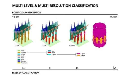
Considering these problems, it becomes difficult to classify very large datasets in one single step, as traditional classification approaches do. Therefore, a multi-level and multi-resolution (MLMR) approach is proposed (Figure 5), which follows these steps:
- The full-resolution point cloud is subsampled in various geometric levels.
- Given certain manually annotated areas corresponding to the classes of interest of the first geometric level, a RF model is trained and then all classes are predicted on the entire point cloud.
- Classification results coming from this first step are back interpolated (BI) on a higher resolution version of the dataset, using a nearest neighbourhood algorithm. To do so, the class value assigned to each point is transferred to a certain number of elements evaluated inside a specific cluster; the number of nearest neighbourhoods to be evaluated depends on the point cloud resolution. The higher the resolution, the higher the number of points in the neighbourhood.
- The next geometric level is considered with its new classes (e.g., columns are divided in base, shaft and capitals) and a new classification procedure is applied.
- Classification results are again back interpolated on a higher resolution version of the point cloud until the full geometric resolution is reached.
It should be mentioned that each architectural element can be classified in more and more details, according to the employed point cloud resolution at the corresponding level, and then back interpolated on a higher resolution version. The process is iterative, and the last classification level will correspond to the full-resolution point cloud. Moreover, the subsampling of the point cloud will depend on both the complexity of the object to be classified and the elements to be recognised. Macro-categories of objects allow for a lower resolution, while the higher resolution is used for details.
The proposed hierarchical methodology is graphically summarised in Figure 5. The diagram aims also to provide for a general indication in terms of geometric resolution of the point cloud and geometric feature ready to be used at each classification step. These values, and the methodology itself, can be considered sufficiently generalisable to be used for the classification of architectural elements in the monumental field. The parameters (resolution and feature radii) can vary case by case according to the characteristics and dimensions of the objects. However, it can be seen that they correspond to the smallest detail that can be represented at a given representation scale and its metric tolerance, in a logic of representation at an increasing level of detail.
As a final and additional step, after the full classification of the point cloud, it is possible to apply the so-called instance segmentation to each architectural class. In this way, for example, each column of the dataset can have its own index. To do so, the label connected component function available in CloudCompare [55] was used. Still, instead of working on pixels arranged in a grid, the octree structure of the point cloud from which it defines the grid step is used to perform the search in the 3D space. The tool separates the cloud into smaller ones based on a minimum distance between elements and a minimum number of points that a component must have.
5. Semantic Classes and Classification Levels
5.1. Milan Cathedral
Following the Veneranda Fabbrica conservation and restoration rules as well as the hierarchical subdivision of the monument in areas, zones, sectors, architectural elements and marble blocks reported in [56], we consider an automatic classification of the cathedral into three different levels (Figure 6).
The first level of classification has the function to identify macro-architectonic elements. The classification process is performed on the point cloud at a 5-cm resolution, extracting geometric features with radii between 20 cm and 2.5 m.
In the second level of classification, the previously identified architectural elements are divided into sub-components (e.g., columns are split in its bases, capitals and shafts). This step is performed using a 2-cm resolution point cloud, reducing to 10 cm and 1 m the min/max feature search radii.
Finally, the third and most challenging level of classification aims at the subdivision of each component in its ashlars (i.e., monolith elements as statues, gothic decoration, holes, etc.). For this, the full resolution point cloud is used with a min and max search radius of 0.5 and 5 cm, respectively.
5.2. Pomposa Abbey
Considering monitoring needs, the classification has been subdivided into three different levels (Figure 7).
The first level refers to the main structural framework of the church, defining a global functional subdivision of the entire dataset: floor, façades, columns, arches, and roof. In order to recognise these macro-categories, the point cloud has been processed at a 5-cm resolution.
The second level is devoted to a more in-depth classification process, recognising multiple sub-classes within the categories coming from the first level of classification. Façades are divided into walls and windows, columns into bases, shafts and capitals, and roof are broken down into dome, side, central and front cover. At this level, each architectural element was recognised at the 2-cm resolution point cloud.
The third level refers to the roof which presents complex and variable structures. A diverse classification process was run for each different roof structure, highlighting its main structural elements (e.g., rafters, purlins, panels, tie beams, wall plates, crown posts, etc.). To finalise this structural study, the suitable resolution of the point cloud was 2 cm.
6. Data Processing
6.1. Geometric Features Extraction
The necessary features for the classification are based on the covariance matrix [57] computed within a local neighbourhood of a 3D point. For both case studies, the considered local neighbourhoods are directly related to the dimension of the architectural elements. Moreover, as various features affect the classification results in different ways, the geometric features with the smallest impact on the training process have been iteratively removed [33]. The experiments showed that, independently from the object to be classified and the point cloud resolution, the features with a more significant impact on the classification results are (Figure 8):
- Anisotropy: allows the recognition of 3D elements such as columns, buttresses and spires over 2.5D elements such as walls and vaults.
- Planarity: highlight linear and planar items such as chains and floors and their vertical counterparts such as column shaft and walls.
- Linearity: similarly to planarity, it helps in identifying linear structures.
- Surface variation: it emphasises changes in the shapes allowing, for example, to detect corners or edges.
- Sphericity: similarly to surface variation, it helps in identifying spherical and cylindrical elements, such as columns.
- Verticality: it points out vertical and horizontal surfaces allowing the recognition of walls and floors as well as column shafts.
Among these covariance features, planarity and linearity, and surface variation and sphericity behave pairwise similarly. However, all of them have been used at the same time to improve the performance of the RF classifier. In fact, as the algorithm splits all the available information among its decision trees, redundancy in geometric features allows us to have the correct relations in every tree, allowing for a better classification.
6.2. Training and Classification
Beside extracting geometric features, some portion of each dataset—at each classification level—has been manually annotated in order to train the RF algorithm. Figure 9 and Figure 10 show the training sets used at the first level of classification (5-cm resolution) of Milan Cathedral and Pomposa Abbey, respectively. For the first case study (30 mil. points), the training sample is composed of ca 2.5 mil. annotated points for the exterior surfaces and ca 2.6 mil. points for the interior spaces. For the Pomposa Abbey, some 115,444 points are used for the training set out of ca 1.1 mil. points composing the whole cloud.
Table 3 reports numbers of used points in the training and classification times for all three classification levels. Figure 11 indicates the percentage of time spent in each working phase. It is important to say that the computation time for the extraction of the geometric features varies in relation to the dimension of the point cloud, the number of features and their search radius. Even if the processing time increases with the dimension of a given training sample, it can still be considered negligible if compared to DL approaches. Regarding the first level of classification, on an 18-core processor workstation, the training phase for the Milan Cathedral took about 5 min (2.5 mil. points), while 43 s were necessary to classify the remaining exterior point cloud (12 mil. points). With regards to the Pomposa Abbey, the training and classification processes took 5 and 3 s, respectively.
7. Results and Discussion
Considering the reduced dimension of the manually annotated portions used to train the classifier, the achieved results in both case studies were successful (Table 4 and Table 7). The metrics used to evaluate these results are Precision, Recall and F1-score. They were computed by comparing, for each dataset, a manually annotated portion with the same portion automatically predicted.
In the next sections, the achieved results will be discussed, focussing on advantages and criticalities related to the semantic segmentation of such complex architectures. Section 7.1.1 and Section 7.2.1 will show the classification results achieved with a traditional classification approach (non-hierarchical, but in one step with all semantic classes) in comparison to the proposed MLMR method.
7.1. Milan Cathedral
7.1.1. One-Step Classification
The Cathedral dataset was classified in one step using a Random Forest method and all 18 semantic classes (see Figures 13 and 14). To perform a one-step (non-hierarchical) classification, due to the huge dimension of the dataset (more than 3 bil. points), the data were subsampled at a 5-cm resolution, unavoidably lowering its details. The training dataset contained all 18 classes and the classification result got an average F1-score of 67%. Results (Figure 12) show that with this approach it is difficult to distinguish elements with similar geometry but belonging to different classes (e.g., ornaments on the capitals of the main nave and ornaments on the choir area). Furthermore, many detailed elements present discontinuities that are equal or smaller than 5 cm, making their recognition complicated.
Therefore, dividing the classification into different geometric levels facilitates the distinction of similar elements as well as allows to process only specific parts of the dataset at the full 5-mm resolution.
7.1.2. MLMR Classification
Figure 13 and Figure 14 show some examples of the subsequent levels of classification, relative to both Cathedral interiors and exteriors. Table 4 shows an average of the F1-score values, computed at each classification level. The classification results, applied to the whole dataset, are shown in Figure 15.
At the first level of classification, it was possible to identify the main elements of the construction visible in a 5-cm resolution point cloud (i.e., for the interior: floors, columns, chains, vaults, walls, and choir; for the exterior: walls, buttresses, roofs, and street). The use of a low-resolution point cloud allowed us to process the whole dataset at once. This kind of operation would have been critical from the hardware and computation point of view if using the full resolution point clouds. In Table 5 and Table 6, it is possible to observe the classification metrics achieved per class in the first level of classification (level 1).
The main classification errors in the first level of classification were due to the following areas: (i) too small with respect to the resolution level, (ii) ambiguous from a geometrical point of view, or (iii) too similar to elements belonging to a different class. For example, it has been difficult to classify chains, which are approximately 8 cm thick, at a 5-cm resolution point clouds.
A second type of problem was found in the area which surrounds the choir. The class choir comprises different architectural elements including pipe organs, benches and altars. The decision to classify them in one class is coherent with the Veneranda Fabbrica rules. However, the heterogeneity of its parts and noise in the 3D point model caused classification problems in neighbouring regions. In fact, as the RF classifier relies on geometrical features of the local points to classify them, it was not able to easily distinguish classes with similar characteristics. An analogue issue has been encountered on the outside part of the Cathedral. Here, the RF classifier could classify only those buttresses that were entirely surveyed. Errors appeared in those parts where, due to building site requirements, it was impossible to survey one of the two buttresses’ faces. In that case, the classifier confused the buttresses with walls, both being 2.5D. In Figure 16, it is possible to see the different behaviour of the same geometric features on complete and incomplete elements.
Before transferring the classification results from levels 1 to 2, misclassification errors have been manually adjusted. In fact, errors at top levels would severely affect classification at the subsequent, more detailed steps.
At the second level of classification, the precision of the results increased (see also Table 4) as the geometric resolution of the point cloud increased. This allowed to identify more peculiar architectural elements. Finally, the third classification level (5-mm resolution) included the most complex shapes to be classified (e.g., statues incorporated inside the capitals): the accuracy metrics slightly decreased due to the complex shapes but also the presence of occlusions in the point clouds as well as geometric similarities between elements (e.g., statues and gothic pyramids).
The final step of the classification process was the instance segmentation, applied to all the single and repeated elements belonging to the same classes (Figure 17 and Figure 18). The instance segmentation allowed to associate a different index to an architectural component of the same class (e.g., statues, capitals, bases, shafts, etc.). This indexing allows for (i) a better management in a HBIM context and (ii) a quick and precise identification of the elements on which to intervene (in accordance to Veneranda Fabbrica intervention rules).
7.2. Pomposa Abbey
7.2.1. One Step Classification
A traditional non-hierarchical classification was applied to the Abbey dataset searching for 18 classes of architectural interest (see Figure 21). Results, shown in Figure 19, seems quite encouraging, with an average F1-score of 75%. However, in order to be used in daily practice, the classification results need some manual misclassification adjustments (Figure 20). The relative acceptable results can be explained by the fact that Pomposa Abbey, even if complex, present less ambiguity among classes with respect to the Milan’s Cathedral. The RF can distinguish among walls and structural parts in the trusses because they are geometrically different (contrary to the statues on the choir and those on the capitals in Milan’s Cathedral). Moreover, the point cloud resolution is low and does not necessarily requires an initial subsampling step.
7.2.2. MLMR classification
The developed MLMR classification approach was applied with three levels (Figure 21). Table 7 reports the F1-scores achieved in the three levels, with an accuracy always over 90%. Working on different levels has facilitated the process of architectural content recognition, avoiding errors that are common when more classes share the same properties (e.g., columns and crown posts). The slight decrease in accuracy for level 3 is due to the fact that, despite an increase of the classes (from 9 to 18), the geometric resolution of the point cloud is like level 2 (2 cm).
At the first classification level, the most complex parts to classify were those columns that are directly inserted in the transverse walls. As shown in Figure 22a, geometric features such as planarity or linearity, that generally help in highlighting columns, responded differently on columns and semi-columns. Still, the integration with other covariance features, such as Surface Variation (Figure 22b), allows quite precise identification of semi-columns.
Once columns and semi-columns have been isolated (Figure 23), the subsequent level of classification, based on a higher resolution, allowed the identification of further elements and details, such as base, capital, shaft, etc. (Figure 24).
The second classification level split the roof into the dome, central, front and side cover, as each part presents a different structural behaviour. Therefore, these roof parts and wooden structures were considered in the last classification level. The parts could be further subdivided, extracting all their various components (Figure 25), but using specific features for each part.
In all cases, the Surface Variation, extracted at radii proportional to the size of the beams, has been essential to highlight the various elements. But, after a strategic re-orientation of the parts, the X and Y coordinates were used as features for the central and front cover, respectively, to distinguish the principal rafters. This latter strategy allowed us to notice the presence of deformations in the central cover, starting from the observation of some anomalies in the classification results (Figure 26).
With regards to the side cover classification, in early stages of experimentation, different problems were encountered as complete and incomplete beams (coming from occlusions in the dataset) responded differently to the feature extraction (Figure 27a). To cope with this issue, a temporary rotation was applied to the side covers, to make them horizontal, so that we could benefit from the Z coordinates for distinguishing rafters, purlins, and panels (Figure 27b,c).
Classification metrics per classes at level 3 are reported in Table 8, Table 9 and Table 10. This level includes very fine details of the roof (purlins, tie beams, etc.) which were classified at the same geometric detail of level 2; hence, the reached accuracy metrics are slightly worse.
Finally, the instance segmentation of the whole wooden roof (Figure 28) provided additional results useful for conservation and monitoring activities, allowing to identify components that have to be replaced. Moreover, the abstraction of structural elements could become preliminary to simulations with finite element methods/analysis systems (FEM/FEA).
8. Conclusions
The paper presented a new hierarchical classification procedure (MLMR) to semantically enrich 3D point clouds of complex heritage structures. The achieved classification results show how enriched point clouds could support a better understanding of complex heritage architectures as well as operations like restoration, communication and on-site facility management. The cognitive contribution of an expert operator is fundamental at the beginning of the process. The following are still required from an expert operator: (i) the identification of the classification rules, (ii) the class definition, and (iii) the choice of training and validation sets (data annotation). These steps are crucial to adapt the process to different case studies.
The innovative aspects of the presented work are as follows:
- The use of machine learning techniques to quickly classify large and complex 3D architectures without the need of large training datasets.
- The definition of general rules (e.g., identification of geometric features), replicable in various heritage scenarios, in terms of relations among classification levels, point cloud resolution and minimum/maximum feature search radii.
- The hierarchical segmentation (until single instances) of 3D surveying data which could facilitate HBIM processes.
- The speed of the process: once training and validation sets are defined, the prediction to the entire dataset is achieved in a few minutes.
- The objectivity of the classification procedure: objective rules are applied uniformly throughout the entire process, making the process repeatable and independent from subjective choices of an operator.
As possible lines of future research, some aspects may deserve further attention and development:
- Better investigation of the relationship between classification levels, point cloud resolution and features search radii: it is necessary to understand if the automatic classification with specific features can be generalised concerning data density, or if it is case dependent.
- Verification of the usefulness of the classification process for the scan-to-BIM process, checking if the extracted semantic structures and instances facilitate the preparatory work for the construction of BIM models.
- Checking if the semantically segmented point clouds could facilitate the generation of polygonal meshes.
- Extension of the instance segmentation, not only to repeated and separated elements but also to those classes that present differences in composition or material, even if contiguous and similar in shape (e.g., walls).
- Creation of a more user-friendly classification framework to be used by non-experts in the sector.
- Testing the possibility to automatically process the data acquired on-site with mobile scanner instruments for real-time monitoring applications.
- Improvement of the classification details by integrating information coming from images, which generally feature higher resolution, hence allows for a better identification/distinction of small elements (e.g., classification of each single marble block composing the Milan Cathedral).
Author Contributions
The article presents a research contribution that involved all authors in equal measure, starting from a 3D dataset acquired by different research groups. In drafting preparation, F.R. supervised the overall work, writing the introduction, aim and conclusions of the paper; S.T. and E.G. dealt with the state of the art, methodology, data processing and results; F.F. was responsible of Milan Cathedral description, paper conclusions and methodology generalisation; M.R. dealt with Pomposa Abbey description, paper introduction and conclusions. All authors have read and agreed to the published version of the manuscript.
Funding
This research partially received external funding from the project "Artificial Intelligence for Cultural Heritage" (AI4CH) joint Italy-Israel lab which was funded by the Italian Ministry of Foreign Affairs and International Cooperation (MAECI).
Acknowledgments
The paper is partially funded by the the project “Artificial Intelligence for Cultural Heritage” (AI4CH), a joint Italy–Israel lab which was funded by the Italian Ministry of Foreign Affairs and International Cooperation (MAECI). The authors are thankful to all participants in the surveying acquisition campaigns and data processing of the two case studies. A special thank goes to A.M. Manferdini for her contribution in the survey and data analysis of the Pomposa Abbey. The authors would also thank the Veneranda Fabbrica del Duomo di Milano and its director Eng. Francesco Canali for his support and availability to allow our research activities.
Conflicts of Interest
The authors declare no conflict of interest.
References
- Remondino, F.; Georgopoulos, A.; Agrafiotis, P. Latest Developments in Reality-Based 3D Surveying and Modelling; MDPI AG: Basel, Switzerland, 2018. [Google Scholar] [CrossRef]
- Gonzalez-Aguilera, D.; Remondino, F.; Nocerino, E. Remote Sensed Data and Processing Methodologies for 3D Virtual Reconstruction and Visualization of Complex Architectures; MDPI AG: Basel, Switzerland, 2016. [Google Scholar] [CrossRef] [Green Version]
- Apollonio, F.I.; Basilissi, V.; Callieri, M.; Dellepiane, M.; Gaiani, M.; Ponchio, F.; Rizzo, F.; Rubino, A.R.; Scopigno, R.; Sobra’, G. A 3D-centered information system for the documentation of a complex restoration intervention. J. Cult. Herit. 2018, 29, 89–99. [Google Scholar] [CrossRef]
- Nocerino, E.; Menna, F.; Toschi, I.; Morabito, D.; Remondino, F.; Rodriguez-Gonzalvez, P. Valorisation of history and landscape for promoting the memory of WWI. J. Cult. Herit. 2018, 29, 113–122. [Google Scholar] [CrossRef] [Green Version]
- Malinverni, E.S.; Pierdicca, R.; Paolanti, M.; Martini, M.; Morbidoni, C.; Matrone, F.; Lingua, A. Deep learning for semantic segmentation of 3D point cloud. ISPRS—Int. Arch. Photogramm. Remote Sens. Spat. Inf. Sci. 2019, XLII-2/W15, 735–742. [Google Scholar] [CrossRef] [Green Version]
- Roussel, R.; Bagnéris, M.; De Luca, L.; Bomblet, P. A digital diagnosis for the « Autumn » statue (Marseille, France): Photogrammetry, digital cartography and construction of a thesaurus. ISPRS—Int. Arch. Photogramm. Remote Sens. Spat. Inf. Sci. 2019, XLII-2/W15, 1039–1046. [Google Scholar] [CrossRef] [Green Version]
- Grilli, E.; Menna, F.; Remondino, F. A review of point clouds segmentation and classification Algorithms. ISPRS—Int. Arch. Photogramm. Remote Sens. Spat. Inf. Sci. 2017, XLII-2/W3, 339–344. [Google Scholar] [CrossRef] [Green Version]
- Griffiths, D.; Boehm, J. A Review on Deep Learning Techniques for 3D Sensed Data Classification. Remote Sens. 2019, 11, 1499. [Google Scholar] [CrossRef] [Green Version]
- Maturana, D.; Scherer, S. VoxNet: A 3D Convolutional Neural Network for real-time object recognition. In Proceedings of the 2015 IEEE/RSJ International Conference on Intelligent Robots and Systems (IROS), Hamburg, Germany, 28 September–2 October 2015; pp. 922–928. [Google Scholar] [CrossRef]
- Jiang, H.; Yan, F.; Cai, J.; Zheng, J.; Xiao, J. End-to-end 3D Point Cloud Instance Segmentation without Detection. In Proceedings of the IEEE/CVF Conference on Computer Vision and Pattern Recognition, Washington, DC, USA, 16–18 June 2020; pp. 12796–12805. [Google Scholar]
- Milioto, A.; Lottes, P.; Stachniss, C. Real-Time Semantic Segmentation of Crop and Weed for Precision Agriculture Robots Leveraging Background Knowledge in CNNs. In Proceedings of the IEEE International Conference on Robotics and Automation, Brisbane, Australia, 21–25 May 2018. [Google Scholar] [CrossRef] [Green Version]
- Wang, L.; Zhang, Y.; Wang, J. Map-Based Localization Method for Autonomous Vehicles Using 3D-LIDAR. In IFAC-PapersOnLine; Elsevier: Amsterdam, The Netherlands, 2017; Volume 50, pp. 276–281. [Google Scholar] [CrossRef]
- Hu, Q.; Yang, B.; Xie, L.; Rosa, S.; Guo, Y.; Wang, Z.; Trigoni, N.; Markham, A. RandLA-Net: Efficient Semantic Segmentation of Large-Scale Point Clouds. In Proceedings of the IEEE/CVF Conference on Computer Vision and Pattern Recognition, Seattle, DC, USA, 16–18 June 2020; pp. 11108–11117. [Google Scholar]
- Kim, W.; Seok, J. Indoor Semantic Segmentation for Robot Navigating on Mobile. In Proceedings of the International Conference on Ubiquitous and Future Networks, Prague, Czech Republic, 3–6 July 2018; pp. 22–25. [Google Scholar] [CrossRef]
- Poux, F.; Billen, R. Voxel-based 3D Point Cloud Semantic Segmentation: Unsupervised Geometric and Relationship Featuring vs Deep Learning Methods. ISPRS Int. J. Geo-Inf. 2019, 8, 213. [Google Scholar] [CrossRef] [Green Version]
- Xu, S.; Vosselman, G.; Elberink, S.O. Multiple-entity based classification of airborne laser scanning data in urban areas. ISPRS J. Photogramm. Remote Sens. 2014, 88, 1–15. [Google Scholar] [CrossRef]
- Zhu, Q.; Li, Y.; Hu, H.; Wu, B. Robust point cloud classification based on multi-level semantic relationships for urban scenes. ISPRS J. Photogramm. Remote Sens. 2017, 129, 86–102. [Google Scholar] [CrossRef]
- Weinmann, M.; Schmidt, A.; Mallet, C.; Hinz, S.; Rottensteiner, F.; Jutzi, B. Contextual classification of point cloud data by exploiting individual 3D neigbourhoods. ISPRS Ann. Photogramm. Remote Sens. Spat. Inf. Sci. 2015, II-3/W4, 271–278. [Google Scholar] [CrossRef] [Green Version]
- Özdemir, E.; Remondino, F.; Golkar, A. Aerial point cloud classification with deep learning and machine learning algorithms. Int. Arch. Photogramm. Remote Sens. Spat. Inf. Sci. 2019, 42, 843–849. [Google Scholar] [CrossRef] [Green Version]
- Grilli, E.; Remondino, F. Classification of 3D Digital Heritage. Remote Sens. 2019, 11, 847. [Google Scholar] [CrossRef] [Green Version]
- Grilli, E.; Dininno, D.; Petrucci, G.; Remondino, F. From 2D to 3D supervised segmentation and classification for cultural heritage applications. ISPRS—Int. Arch. Photogramm. Remote Sens. Spat. Inf. Sci. 2018, 2, 399–406. [Google Scholar] [CrossRef] [Green Version]
- Son, H.; Kim, C. Semantic As-built 3D Modeling of Structural Elements of Buildings based on Local Concavity and Convexity. In Advanced Engineering Informatics; Elsevier: Amsterdam, The Netherlands, 2017; Volume 34, pp. 114–124. [Google Scholar] [CrossRef]
- Lu, Q.; Lee, S. Image-based technologies for constructing as-is building information models for existing buildings. J. Comput. Civ. Eng. 2017, 31, 04017005. [Google Scholar] [CrossRef]
- Rebolj, D.; Pučko, Z.; Babič, N.Č.; Bizjak, M.; Mongus, D. Point cloud quality requirements for Scan-vs-BIM based automated construction progress monitoring. Autom. Constr. 2017, 84, 323–334. [Google Scholar] [CrossRef]
- Bassier, M.; Yousefzadeh, M.; Vergauwen, M. Comparison of 2D and 3D wall reconstruction algorithms from point cloud data for as-built BIM. J. Inf. Technol. Constr. 2020, 25, 173–192. [Google Scholar] [CrossRef]
- Valero, E.; Bosche, F.; Forster, A.M. Automatic segmentation of 3D point clouds of rubble masonry walls, and its application to building surveying, repair and maintenance. Autom. Constr. 2018, 96, 29–39. [Google Scholar] [CrossRef]
- Sánchez-Aparicio, L.J.; Del Pozo, S.; Ramos, L.F.; Arce, A.; Fernandes, F. Heritage site preservation with combined radiometric and geometric analysis of TLS data. Autom. Constr. 2018, 85, 24–39. [Google Scholar] [CrossRef]
- Bosché, F. Automated Recognition of 3D CAD Model objects in Laser Scans and Calculation of As-built Dimensions for Dimensional Compliance Control in Construction. In Advanced Engineering Informatics; Elsevier: Amsterdam, The Netherlands, 2010; Volume 24, pp. 107–118. [Google Scholar] [CrossRef]
- Ordóñez, C.; Martínez, J.; Arias, P.; Armesto, J.; Martinez-Sanchez, J. Measuring building façades with a low-cost close-range photogrammetry system. Autom. Constr. 2010, 19, 742–749. [Google Scholar] [CrossRef]
- Mizoguchi, T.; Koda, Y.; Iwaki, I.; Wakabayashi, H.; Kobayashi, Y.; Shirai, K.; Hara, Y.; Lee, H.-S. Quantitative scaling evaluation of concrete structures based on terrestrial laser scanning. Autom. Constr. 2013, 35, 263–274. [Google Scholar] [CrossRef]
- Kashani, A.G.; Graettinger, A.J. Cluster-Based Roof Covering Damage Detection in Ground-Based Lidar Data. Autom. Constr. 2015, 58, 19–27. [Google Scholar] [CrossRef]
- Murtiyoso, A.; Grussenmeyer, P. Virtual Disassembling of Historical Edifices: Experiments and Assessments of an Automatic Approach for Classifying Multi-Scalar Point Clouds into Architectural Elements. Sensors 2020, 20, 2161. [Google Scholar] [CrossRef] [PubMed] [Green Version]
- Grilli, E.; Farella, E.M.; Torresani, A.; Remondino, F. Geometric features analysis for the classification of cultural heritage point clouds. ISPRS—Int. Arch. Photogramm. Remote Sens. Spat. Inf. Sci. 2019, XLII-2/W, 541–548. [Google Scholar] [CrossRef] [Green Version]
- Grilli, E.; Remondino, F. Machine Learning Generalisation across Different 3D Architectural Heritage. ISPRS Int. J Geo-Inf. 2020, 9, 379. [Google Scholar] [CrossRef]
- Llamas, J.; Lerones, P.M.; Medina, R.; Zalama, E.; García-Bermejo, J.G. Classification of Architectural Heritage Images Using Deep Learning Techniques. Appl. Sci. 2017, 7, 992. [Google Scholar] [CrossRef] [Green Version]
- Yasser, A.M.; Clawson, K.; Bowerman, C.; Mustafá, Y. Saving cultural heritage with digital make-believe: Machine learning and digital techniques to the rescue. In Proceedings of the 31st British Computer Society Human Computer Interaction Conference, Sunderland, UK, 3–6 July 2017; pp. 97–101. [Google Scholar] [CrossRef]
- Charles, R.Q.; Su, H.; Kaichun, M.; Guibas, L.J. PointNet: Deep Learning on Point Sets for 3D Classification and Segmentation. In Proceedings of the Conference on Computer Vision and Pattern Recognition (CVPR), Honolulu, HI, USA, 21–26 July 2017; pp. 77–85. [Google Scholar] [CrossRef] [Green Version]
- Qi, C.R.; Yi, L.; Su, H.; Guibas, L.J. PointNet++: Deep Hierarchical Feature Learning on Point Sets in a Metric Space. In Proceedings of the Conference on Neural Information Processing Systems (NIPS), Long Beach, CA, USA, 24 January 2019. [Google Scholar]
- Pierdicca, R.; Paolanti, M.; Matrone, F.; Martini, M.; Morbidoni, C.; Malinverni, E.S.; Frontoni, E.; Lingua, A.M. Point Cloud Semantic Segmentation Using a Deep Learning Framework for Cultural Heritage. Remote Sens. 2020, 12, 1005. [Google Scholar] [CrossRef] [Green Version]
- Matrone, F.; Lingua, A.; Pierdicca, R.; Malinverni, E.S.; Paolanti, M.; Grilli, E.; Remondino, F.; Murtiyoso, A.; Landes, T. A benchmark for large-scale heritage point cloud semantic segmentation. ISPRS—Int. Arch. Photogramm. Remote Sens. Spat. Inf. Sci. 2020, XLIII-B2, 4558–4567. [Google Scholar]
- Grilli, E.; Özdemir, E.; Remondino, F. Application of machine and deep learning strategies for the classification of heritage point clouds. ISPRS—Int. Arch. Photogramm. Remote Sens. Spat. Inf. Sci. 2019, XLII-4/W18, 447–454. [Google Scholar] [CrossRef] [Green Version]
- Fassi, F.; Achille, C.; Fregonese, L. Surveying and modelling the main spire of Milan Cathedral using multiple data sources. Photogramm. Rec. 2011, 26, 462–487. [Google Scholar] [CrossRef]
- Achille, C.; Fassi, F.; Mandelli, A.; Perfetti, L.; Rechichi, F.; Teruggi, S. From A Traditional to A Digital Site: 2008–2019. The History of Milan Cathedral Surveys. In Research for Development; Springer: Berlin/Heidelberg, Germany, 2020; pp. 331–341. [Google Scholar] [CrossRef] [Green Version]
- Perfetti, L.; Fassi, F.; Gulsan, H. Generation of gigapixel orthophoto for the maintenance of complex buildings. Challenges and lesson learnt. ISPRS—Int. Arch. Photogramm. Remote Sens. Spat. Inf. Sci. 2019, 42, 605–614. [Google Scholar] [CrossRef] [Green Version]
- Perfetti, L.; Polari, C.; Fassi, F. Fisheye photogrammetry: Tests and methodologies for the survey of narrow spaces. ISPRS—Int. Arch. Photogramm. Remote Sens. Spat. Inf. Sci. 2017, 42, 573–580. [Google Scholar] [CrossRef] [Green Version]
- Mandelli, A.; Fassi, F.; Perfetti, L.; Polari, C. Testing different survey techniques to model architectonic narrow spaces. ISPRS—Int. Arch. Photogramm. Remote Sens. Spat. Inf. Sci. 2017, XLII-2/W5, 505–511. [Google Scholar] [CrossRef] [Green Version]
- Salmi, M. L’abbazia Di Pomposa; Amilcare Pizzi: Milano, Italy, 1966. [Google Scholar]
- Russo, E. Profilo Storico-artistico Della Chiesa Abbaziale di Pomposa. In L’arte sacra nei Ducati Estensi, Proceedings of the II Settimana Dei Beni Storico-Artistici Della Chiesa Nazionale Negli Antichi Ducati Estensi, Ferrara, Italy, 13–18 September 1982; Fellani, G., Ed.; Sate: Ferrara, Italy, 1984. [Google Scholar]
- Addison, A.; Gaiani, M. Virtualized architectural heritage: New tools and techniques. IEEE MultiMedia 2000, 7, 26–31. [Google Scholar] [CrossRef]
- El-Hakim, S.F.; Beraldin, J.A.; Picard, M.; Vettore, A. Effective 3d modeling of heritage sites. In Proceedings of the Fourth International Conference on 3-D Digital Imaging and Modeling, 2003. 3DIM 2003, Banff, AB, Canada, 6–10 October 2003; IEEE: Piscataway, NJ, USA; pp. 302–309. [Google Scholar] [CrossRef] [Green Version]
- Cosmi, E.; Guerzoni, G.; Di Francesco, C.; Alessandri, C. Pomposa Abbey: FEM Simulation of Some Structural Damages and Restoration Proposals. In Structural Studies, Repairs and Maintenance of Historical Buildings, WIT Transaction of The Built Environment; Brebbia, C.A., Ed.; WIT Press: Wessex, UK, 1999; Volume 42. [Google Scholar] [CrossRef]
- Francesco, C.; Di Mezzadri, G. Indagini e Rilievi per Interventi Strutturali Nella Chiesa Abbaziale di Santa Maria di Pomposa. In Il Cantiere Della Conoscenza, Il Cantiere Del Restauro, Proceedings of Convegno Di Studi, Bressanone, Italy, 27–30 June 1989; Biscontin, G., Dal Colle, M., Volpin, S., Eds.; Libreria Progetto: Bressanone, Italy, 1989. [Google Scholar]
- Russo, M.; Manferdini, A.M. Integration of image and range-based techniques for surveying complex architectures. ISPRS Ann. Photogramm. Remote Sens. Spat. Inf. Sci. 2014, 2, 305–312. [Google Scholar] [CrossRef] [Green Version]
- Breiman, L. Random Forest. Mach. Learn. 2001, 45, 5–32. [Google Scholar] [CrossRef] [Green Version]
- Cloud Compare (Version 2.11.0) [GPL software]. Available online: http://www.cloudcompare.org/ (accessed on 3 August 2020).
- Fassi, F.; Parri, S. Complex Architecture in 3D: From Survey to Web. Int. J. Herit. Digit. Era 2012, 1, 379–398. [Google Scholar] [CrossRef]
- Chehata, N.; Guo, L.; Mallet, C. Airborne lidar feature selection for urban classification using random forests. Laser Scanning 2009 IAPRS 2009, XXXVIII, 207–212. Available online: https://hal.archives-ouvertes.fr/hal-02384719/ (accessed on 10 August 2020).
Figure 1.
(a) Milan Cathedral main facade. (b) A detail of the complex roof with repetitive buttresses. (c) Internal view of the main nave and its capitals.
Figure 1.
(a) Milan Cathedral main facade. (b) A detail of the complex roof with repetitive buttresses. (c) Internal view of the main nave and its capitals.

Figure 2.
The entire 3D point cloud of the Milan Cathedral (more than 3 billion points). TLS data are shown with their intensity colours (green, yellow, orange) whereas photogrammetric point clouds have RGB colour information.
Figure 2.
The entire 3D point cloud of the Milan Cathedral (more than 3 billion points). TLS data are shown with their intensity colours (green, yellow, orange) whereas photogrammetric point clouds have RGB colour information.

Figure 3.
Two views of the Abbey complex (a) as seen from a drone/UAS platform. (b) Main nave of the church.
Figure 3.
Two views of the Abbey complex (a) as seen from a drone/UAS platform. (b) Main nave of the church.

Figure 4.
Survey schema of the indoor acquisition campaign and three visualisations of the interior coloured point cloud of the Abbey.
Figure 4.
Survey schema of the indoor acquisition campaign and three visualisations of the interior coloured point cloud of the Abbey.

Figure 5.
Multi-level and multi-resolution (MLMR) workflow. The diagram provides also general indications in terms of point cloud resolution and minimum/maximum search radius of the geometric features, which have to be chosen at each step of the classification process. BI stands for Back Interpolation, i.e., classification results at a certain level are back interpolated to a higher resolution level of the point cloud until the full geometric resolution is reached.

Figure 6.
Classification levels and classes for the Milan Cathedral.

Figure 7.
Classification levels and classes for the Pomposa Abbey.

Figure 8.
Visual comparison of geometric features. The colour of the plot represents the feature scale. The used search radii are reported in brackets.
Figure 8.
Visual comparison of geometric features. The colour of the plot represents the feature scale. The used search radii are reported in brackets.

Figure 9.
Annotated portions at classification level 1 for the Milan Cathedral.

Figure 10.
Annotated portions at classification level 1 for the Pomposa Abbey.

Figure 11.
Comparison of normalized time necessary for the different phases of the classification process, from manual annotation to final classification of the dataset.
Figure 11.
Comparison of normalized time necessary for the different phases of the classification process, from manual annotation to final classification of the dataset.

Figure 12.
Milan’s Cathedral non-hierarchical classification results with 18 classes (average F1-score: 67%).
Figure 12.
Milan’s Cathedral non-hierarchical classification results with 18 classes (average F1-score: 67%).

Figure 13.
MLMR classification levels (till capital details) for the Milan Cathedral.

Figure 14.
MLMR classification levels for the external walls of the Milan Cathedral.

Figure 15.
Classification results (nine classes) at level 1 for the entire Milan Cathedral.

Figure 16.
Different features behaviour on complete and incomplete objects. (a) Surface variation (1.2); (b) Anisotropy (1.4).
Figure 16.
Different features behaviour on complete and incomplete objects. (a) Surface variation (1.2); (b) Anisotropy (1.4).

Figure 17.
Example of instance segmentation on the pillars of the main nave.

Figure 18.
Example of instance segmentation on a capital of the main nave in order to distinguish the various statues (S1, S2, etc.).
Figure 18.
Example of instance segmentation on a capital of the main nave in order to distinguish the various statues (S1, S2, etc.).

Figure 19.
One step (non-hierarchical) classification results for the Pomposa Abbey with 18 classes (average F1-score: 75%).
Figure 19.
One step (non-hierarchical) classification results for the Pomposa Abbey with 18 classes (average F1-score: 75%).

Figure 20.
Misclassification details. (a) Truss. (b) Column.

Figure 21.
MLMR classification (18 classes overall) for the Pomposa Abbey. Please note that tie beam, panel and purlin are repeated among the sub-classes.
Figure 21.
MLMR classification (18 classes overall) for the Pomposa Abbey. Please note that tie beam, panel and purlin are repeated among the sub-classes.

Figure 22.
Different behaviours of geometric features over columns and semi-columns: (a) Planarity (0.6) and (b) Surface variation (0.4).
Figure 22.
Different behaviours of geometric features over columns and semi-columns: (a) Planarity (0.6) and (b) Surface variation (0.4).

Figure 23.
Classification results (five classes) at level 1 for the entire Pomposa abbey.

Figure 24.
Classification results (11 classes) at level 2 for the entire Abbey (a). A closer view of a column with its sub-elements (b).
Figure 24.
Classification results (11 classes) at level 2 for the entire Abbey (a). A closer view of a column with its sub-elements (b).

Figure 25.
Results at classification level 3 for the Pomposa Abbey’s roof: (a) central; (b) front; (c) side cover. Colour legend as in Figure 18.
Figure 25.
Results at classification level 3 for the Pomposa Abbey’s roof: (a) central; (b) front; (c) side cover. Colour legend as in Figure 18.

Figure 26.
Top view with x-axis deviation highlighted and subsequent anomalies in the classification results of the wooden roof. Some closer views: (A) correct; (B) error in properly distinguishing the elements.
Figure 26.
Top view with x-axis deviation highlighted and subsequent anomalies in the classification results of the wooden roof. Some closer views: (A) correct; (B) error in properly distinguishing the elements.

Figure 27.
Bottom-up views with relative sections of the side cover: (a) surface variation behaviour with critical areas highlighted; (b) scalar field of the original and (c) rotated Z coordinates.
Figure 27.
Bottom-up views with relative sections of the side cover: (a) surface variation behaviour with critical areas highlighted; (b) scalar field of the original and (c) rotated Z coordinates.

Figure 28.
Instance segmentation of the roof structures.


Table 1.
Summary of 3D survey data acquisition and process for the Milan Cathedral.
| Architectural Elements | Method | # Acquisitions | # 3D Points | Mean Resol. (mm) | Subsampling (cm) |
|---|---|---|---|---|---|
| External Areas | Photogrammetry, Leica RTC360 | 16,080 photos, 54 scans | 1.5 billion | 5 | 2−5 |
| Internal Spaces | Leica HDS 7000, Leica C10 | 238 scans | 2.1 billion | 5 | 2−5 |
Table 2.
Summary of 3D survey data acquisition and process for the interior of the Pomposa Abbey.
| Architectural Elements | Instruments | # Acquisitions | # 3D Points | Mean Resol. (mm) | Subsampling (cm) |
|---|---|---|---|---|---|
| External Areas | Leica C10 | 21 | 161 mil. | 5, 20 | 2, 5 |
| Internal Spaces | Faro Focus X 120 | 31 | 580 mil. | 10 | 2, 5 |
Table 3.
Examples of training and classification times in relation to the number of used points in some areas of the two case studies.
Table 3.
Examples of training and classification times in relation to the number of used points in some areas of the two case studies.
| Level 1 | Level 2 | Level 3 | ||||
|---|---|---|---|---|---|---|
| Milan Cathedral (Exteriors) | Pomposa Abbey | Milan Cathedral (Pillars) | Pomposa Abbey (Columns) | Milan Cathedral (Capitals) | Pomposa Abbey (Central Roof) | |
| # of Training Points | 2,580,368 | 115,444 | 1,011,994 | 21,389 | 3,309,947 | 62,258 |
| Training Time (Sec) | 363 | 5 | 17 | 0.65 | 142 | 4.25 |
| # of Classified Points | 12,680,681 | 1,102,569 | 14,645,986 | 47,006 | 47,651,835 | 832,549 |
| Classification Time (Sec) | 43.5 | 2.7 | 12.62 | 0.15 | 174.89 | 29.8 |
Table 4.
Milan Cathedral: the F1-scores average values for all three classification levels (in brackets the geometric resolutions of the point clouds). Please consider that each level has a different number of classes.
Table 4.
Milan Cathedral: the F1-scores average values for all three classification levels (in brackets the geometric resolutions of the point clouds). Please consider that each level has a different number of classes.
| Level 1 (5 cm) | Level 2 (2 cm) | Level 3 (0.5 cm) | |
|---|---|---|---|
| F1 (%) | 93.75 | 99.35 | 91.80 |
Table 5.
Classification metrics at level 1 for the interiors of Milan Cathedral.
| Chains | Choir | Walls | Floor | Columns | Vaults | AVERAGE | WEIGHTED AVERAGE | |
|---|---|---|---|---|---|---|---|---|
| PREC. (%) | 67.52 | 85.19 | 94.08 | 98.03 | 90.15 | 98.28 | 88.88 | 93.05 |
| RECALL (%) | 89.96 | 85.41 | 93.42 | 94.37 | 94.85 | 94.54 | 92.09 | 93.05 |
| F1 (%) | 71.14 | 85.30 | 93.75 | 96.17 | 92.45 | 96.37 | 90.46 | 93.02 |
Table 6.
Classification metrics at level 1 for the exteriors of Milan Cathedral.
| Buttresses | Walls | Street | Roofs | AVERAGE | WEIGHTED AVERAGE | |
|---|---|---|---|---|---|---|
| PREC. (%) | 92.75 | 97.34 | 99.66 | 99.03 | 97.19 | 96.44 |
| RECALL (%) | 92.62 | 97.47 | 99.06 | 98.42 | 96.89 | 96.44 |
| F1 (%) | 92.68 | 97.40 | 99.36 | 98.72 | 97.04 | 96.44 |
Table 7.
Pomposa Abbey: the F1-scores average values for all three classification levels (in brackets the geometric resolutions of the point clouds). Please consider that each level has a different number of classes. The classification levels 2 and 3 are performed on the point cloud at a 2-cm resolution, i.e., the native resolution.
| Level 1 (5 cm) | Level 2 (2 cm) | Level 3 (2 cm) | |
|---|---|---|---|
| F1 (%) | 95.1 | 97.8 | 94.6 |
Table 8.
Classification metrics at level 3 for the central cover of the Pomposa Abbey’s roof.
| Purlin | Panel | Wall Plate | Tie Beam | Principal Rafter (Right) | Principal Rafter (Left) | Crown Post | AVERAGE | WEIGHTED AVERAGE | |
|---|---|---|---|---|---|---|---|---|---|
| PREC. (%) | 96.66 | 86.99 | 95.71 | 97.21 | 90.11 | 94.54 | 86.44 | 89.67 | 88.05 |
| RECALL (%) | 61.53 | 92.29 | 95.09 | 97.64 | 92.10 | 93.12 | 89.41 | 88.74 | 89.04 |
| F1 (%) | 68.27 | 89.56 | 95.40 | 97.43 | 91.09 | 93.82 | 87.90 | 89.20 | 88.39 |
Table 9.
Classification metrics at level 3 for the front cover of the Pomposa Abbey’s roof.
| Panel | Purlin | Crown Post | Principal Rafter (Left) | Tie Beam | Principal Rafter (Right) | AVERAGE | WEIGHTED AVERAGE | |
|---|---|---|---|---|---|---|---|---|
| PREC. (%) | 96.86 | 97.13 | 83.87 | 67.36 | 99.57 | 87.52 | 88.72 | 95.77 |
| RECALL (%) | 98.47 | 93.70 | 92.24 | 68.63 | 99.36 | 87.87 | 90.05 | 95.79 |
| F1 (%) | 97.66 | 95.38 | 87.86 | 67.99 | 99.46 | 87.70 | 89.34 | 95.77 |
Table 10.
Classification metrics at level 3 for the side cover of the Pomposa Abbey’s roof.
| Panel | Principal Rafter | Purlin | AVERAGE | WEIGHTED AVERAGE | |
|---|---|---|---|---|---|
| PREC. (%) | 97.25 | 98.41 | 97.7 | 97.79 | 97.46 |
| RECALL (%) | 100.00 | 96.16 | 85.23 | 93.80 | 97.45 |
| F1 (%) | 98.61 | 97.27 | 91.04 | 95.64 | 97.38 |
© 2020 by the authors. Licensee MDPI, Basel, Switzerland. This article is an open access article distributed under the terms and conditions of the Creative Commons Attribution (CC BY) license (http://creativecommons.org/licenses/by/4.0/).
Share and Cite
MDPI and ACS Style
Teruggi, S.; Grilli, E.; Russo, M.; Fassi, F.; Remondino, F. A Hierarchical Machine Learning Approach for Multi-Level and Multi-Resolution 3D Point Cloud Classification. Remote Sens. 2020, 12, 2598. https://doi.org/10.3390/rs12162598
AMA Style
Teruggi S, Grilli E, Russo M, Fassi F, Remondino F. A Hierarchical Machine Learning Approach for Multi-Level and Multi-Resolution 3D Point Cloud Classification. Remote Sensing. 2020; 12(16):2598. https://doi.org/10.3390/rs12162598
Chicago/Turabian StyleTeruggi, Simone, Eleonora Grilli, Michele Russo, Francesco Fassi, and Fabio Remondino. 2020. "A Hierarchical Machine Learning Approach for Multi-Level and Multi-Resolution 3D Point Cloud Classification" Remote Sensing 12, no. 16: 2598. https://doi.org/10.3390/rs12162598
Note that from the first issue of 2016, this journal uses article numbers instead of page numbers. See further details here.