GPU-Based Soil Parameter Parallel Inversion for PolSAR Data

Abstract

With the development of polarimetric synthetic aperture radar (PolSAR), quantitative parameter inversion has been seen great progress, especially in the field of soil parameter inversion, which has achieved good results for applications. However, PolSAR data is also often many terabytes large. This huge amount of data also directly affects the efficiency of the inversion. Therefore, the efficiency of soil moisture and roughness inversion has become a problem in the application of this PolSAR technique. A parallel realization based on a graphics processing unit (GPU) for multiple inversion models of PolSAR data is proposed in this paper. This method utilizes the high-performance parallel computing capability of a GPU to optimize the realization of the surface inversion models for polarimetric SAR data. Three classical forward scattering models and their corresponding inversion algorithms are analyzed. They are different in terms of polarimetric data requirements, application situation, as well as inversion performance. Specifically, the inversion process of PolSAR data is mainly improved by the use of the high concurrent threads of GPU. According to the inversion process, various optimization strategies are applied, such as the parallel task allocation, and optimizations of instruction level, data storage, data transmission between CPU and GPU. The advantages of a GPU in processing computationally-intensive data are shown in the data experiments, where the efficiency of soil roughness and moisture inversion is increased by one or two orders of magnitude.

1. Introduction

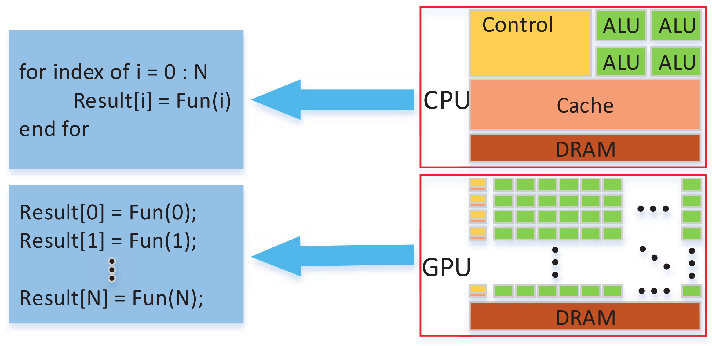
Soil moisture and roughness are important parameters in the fields of agriculture, ecology, meteorology, and hydrology. They are widely used in farmland irrigation management, climate prediction, and drought monitoring [1]. For example, in the agricultural area, soil water content and roughness directly affect crop growth [2]. The correct assessment of soil moisture is also the basis of hydrological modeling [3]. In the meteorological field, soil water content is an essential component of the land–atmosphere boundary energy budget [4,5]. Therefore, the inversion of soil water content and roughness has become a research hotspot for scholars.

With the increase in the number of global satellites, the application of ground exploration has become increasingly common [6,7,8]. But low resolution is also a major problem for exploration [9,10]. The development of science and technology has promoted the rapid development of synthetic aperture radar (SAR) techniques, through which the quality and resolution of radar imaging has been significantly improved. However, in the process of ground detection, the anti-interference of SAR is very low, and the detection process is easily affected. Both GIS and remote sensing assistance information are used for soil moisture estimation [11]. Multi-satellite collaboration can also improve spatio-temporal resolution [12]. By means of dual/multi/full polarization, the polarized synthetic aperture radar (PolSAR) has a good detection effect and high resolution [13]. PolSAR plays an important role in geographic surveying, geological hazard monitoring, vegetation monitoring, and other applications [14]. The applications of PolSAR data can be generally divided into two categories, which are qualitative and quantitative ones. For qualitative applications, the PolSAR technique has a great advantage in unsupervised classification due to the inherent scattering mechanisms contained in PolSAR data. This kind of physical scattering information can be directly used for land cover classification which need no training.

For quantitative applications, PolSAR has a profound impact on the study of parameter inversion. Here PolSAR provides the relations between observations of multi-polarimetric channels with system parameters and object parameters, which is more stable than single polarimetric channel observation. Soil parameter estimation is a representative quantitative application of PolSAR data, since it covers both geometrical and physical parameters. In the study of bare soil parameters, scholars at home and abroad have developed a variety of soil parameter inversion models. These models are broadly divided into theoretical scattering models and empirical scattering models. The theoretical models include physical optics (PO) models, geometrical optics (GO) models, and integral equation methods (IEM). The theoretical models are based on the assumptions that the naturally exposed surface is a uniform half-space dielectric layer, so the accuracy of these models is limited [9,14,15]. Some scholars have studied the accuracy of the inversion model [16,17,18]. However, its complicated form makes it very difficult to obtain the roughness and water content parameters directly from the polarization imagery. Therefore, combining theoretical model analysis and polarization data sets, establishing an empirical relationship between various echo parameters and surface parameters has become the main way to obtain surface parameters [19,20]. The empirical and semi-empirical models include small perturbation methods (SPM), Dubois, Oh, and other models. By comparing the calculated result with the actual external measurement, then with the adjustment of the parameters, the soil parameters calculated by the model are more in line with the actual situation [21]. In order to obtain more accurate results, the X-Bragg model based on full polarization is also proposed. The model is based on the eigenvalues and eigenvectors of the polarization coherence matrix. However, the high-resolution PolSAR massive imagery becomes the bottleneck of computing efficiency.

The efficient processing speed of soil moisture retrieval can help make timely decisions in the real-time application of geological exploration [4]. In recent years, the development of high-performance technologies has solved the computing-intensive problem, especially the GPU parallel method, e.g., hybrid OpenMP-CUDA based PDE source inversion [22], multiplication regular comparison source (MR-CSI) graphic processing unit (GPU) parallel optimization [23], GPU 2D and 3D multi-frequency regularization comparison source [24], parallel optimization of multi-scale MAS systems, and GPU-based accelerated TMI [25]. Parallel computing research of large-scale grounded grid PC cluster is realized [26]. In the heterogeneous soil model, OpenMP parallel optimization is used for multi-core parallelism implementation [27]. In our previous work, various parallel mechanisms have been introduced to accelerate the SAR raw data simulation, including clouding computing, GPU parallel, CPU parallel, and hybrid CPU/GPU parallel [28,29,30,31,32,33,34,35]. As far as the inversion algorithms are concerned, the time cost is only minute-level. Compared with the hybrid CPU/GPU parallel accelerating, the GPU parallel is expected to be a better choice for balancing the algorithm complexity and efficiency. Therefore, single GPU has been employed to implement the massive parallel parameter inversion for PolSAR imagery.

This paper studies the Dubois, Oh, and X-Bragg model inversion algorithms, which basically covers all widely used empirical models. Among them, the Dubois and Oh models use scattering coefficients of two or three polarimetric channels, which is only the amplitude information, while the X-Bragg model utilizes the full polarimetric scattering matrix including both amplitude and phase information. In fact, the higher data requirement of models has, the better performance it achieves. When the full polarimetric scattering matrix is available, Oh and X-Bragg models can be used. However, for the surface with vegetation and non-unneglectable slope, X-Bragg model should be chosen with priority. When we have amplitude data of polarimetric channels, Dubois and Oh models could be employed. In the case that only dual polarimetric data is available (HH,VV), then the Dubois model is left. It should be noted that with the Dubois model, good results are obtained under the condition that the incidence angle is larger than 30 degrees. The scattering models themselves are a forward model, that is, from the input object parameters and observation parameters to the scattering matrix or coefficients. However, if we want to retrieve the soil roughness and moisture from the data, the corresponding inversion algorithms are needed. We mainly analyze the optimization of the three algorithms for soil inversion based on the GPU parallel method. Therefore, the contributions of this paper are mainly reflected in the parallel design (GPU thread allocation strategy), parallel optimization for computing-intensive issue (instruction optimization), and parallel optimization for data-intensive issue (storage optimization and data type conversion). Through the three aspects of parallel acceleration, $14\times$–$169\times$ speedups can be achieved for the three inversion models.

The rest of this paper is organized as follows. In Section 2, the three inversion algorithms are specifically introduced, including the Dubois model, Oh model, and X-Bragg model. In Section 3, the sequential algorithm analysis and the proposed parallel methods are presented. In Section 4, the experimental results and analysis are presented. The conclusion is given in the final section.

2. Inversion Algorithm

2.1. Dubois Model

In 1995, Dubois proposed an empirical model that only requires the same polarization backscatter coefficients ${\sigma }_{HH}^0$ and ${\sigma }_{VV}^0$ to extract the root mean square height and water content of the bare soil. The model was built using the datasets collected by a truck-mounted scatterometer at the University of Michigan and the RASAM scatterometer at the University of Bern. Through the measurement of the scatterometer and the data, the local incident angle and frequency, the dielectric constant and the surface roughness are mapped to the co-polarized scattering coefficient. Studies have found that this relationship is close to the tangent of the angle of incidence. The algorithm is applied to SAR data (AIRSAR and SIR-C) to prove its robustness [36].

The empirical formula is as follows:

$${\sigma }_{HH}^0={10}^{-2.75}\ast \frac{co{s}^{1.5}\theta }{si{n}^5\theta }\ast {10}^{0.028\ast {\epsilon }_r\ast tan\theta }{(ks\ast sin\theta )}^{1.4}\ast {\lambda }^{0.7}$$

(1)

$${\sigma }_{VV}^0={10}^{-2.37}\ast \frac{co{s}^3\theta }{si{n}^3\theta }\ast {10}^{0.046\ast {\epsilon }_r\ast tan\theta }{(ks\ast sin\theta )}^{1.1}\ast {\lambda }^{0.7}$$

(2)

where $\theta$ is the local incidence angle, ${\epsilon }_r$ is the real part of the dielectric constant, $ks$ the normalized surface roughness and $\lambda$ the wavelength.

The volume water content of soil $m_v$ can be calculated from the relationship between ${\epsilon }_r$ and $m_v$:

$$m_v=4.3\ast {10}^{-6}{\epsilon }_r^3-5.5\ast {10}^{-4}{\epsilon }_r^2+2.92\ast {10}^{-2}{\epsilon }_r-5.3\ast {10}^{-2}$$

(3)

The effective range of the inversion model for estimating surface parameters is $m_v\le 35\%$, $ks\le 2.5$ and $\theta \ge {30}^{\circ }$.

2.2. Oh Model

At the University of Michigan, based on the analysis of the classical theoretical scattering model Kirchhoff approximation (KA) and SPM, Y. Oh, K.Sarabandi, and F.T. Ulaby developed this semi-empirical model in 1992. The model uses full-polarization data (LCX POLARSCAT) measured by an on-board network analysis scatterometer at three frequencies (1.5, 4.5, and 9.5 GHz), as well as comprehensive and accurate surface measurements, with incident angles ranging from ${10}^{\circ }$ to ${70}^{\circ }$ [36,37].

The model proposes a clear cross-polarization and co-polarization backscatter ratio function. The empirical equation is:

$$P=\frac{{\sigma }_{HV}^0}{{\sigma }_{VV}^0}=0.23\sqrt{{\Gamma }^0}(1-e^{-ks})$$

(4)

$$Q=\frac{{\sigma }_{HH}^0}{{\sigma }_{VV}^0}={(1-{(\frac{2\theta }{\pi })}^{\frac{1}{3{\Gamma }^0}}\ast e^{-ks})}^2$$

(5)

where P and Q represent the cross-polarization and co-polarization backscatter ratios (i.e., $\frac{{\sigma }_{HV}^0}{{\sigma }_{VV}^0}$ and $\frac{{\sigma }_{HH}^0}{{\sigma }_{VV}^0}$), $\theta$ is the local incident angle, and $ks$ is the root mean square height (i.e., roughness) after the wavelength is normalized, and ${\Gamma }^0$ is the Fresnel reflection coefficient.

$${\Gamma }^0=\left|\frac{1-\sqrt{{\epsilon }_r}}{1+\sqrt{{\epsilon }_r}}\right|.$$

(6)

By combining Equations (4)–(6) we can obtain the mathematical Equation (7):

$$x^{{}_n}=\frac{a^{\frac{{\left(x_{n-1}\right)}^2}{3}}(1-b{x}_{n-1})+c}{\left[\frac{2x_{n-1}}{3}ln\left(a\right)(1-b{x}_{n-1})-b\right]a^{\frac{{\left(x_{n-1}\right)}^2}{3}}.}$$

(7)

Among them, $x=\frac{1}{{\Gamma }^0}$, $b=\frac{q}{0.23}$, $a=\frac{2\theta }{\pi }$ and $c=\sqrt{p}-1$. x is obtained by the iterative method in the program, and then the Fresnel reflectivity ${\Gamma }^0$ and Fresnel reflection coefficient ${\epsilon }_r$ can be obtained, as well as the soil roughness ($ks$) and soil moisture ($mv$). In general, the model shows good agreement on ground measurements within a certain range, where $ks\in \left[0.1,6\right]$,$m_v\in \left[9,31\right]$.

2.3. X-Bragg Model

X-Bragg model is an SPM-based polarimetric scattering model. It utilizes the coherency matrix of full polarimetric data, including the phase information. Firstly, from the side of polarimetric coherency matrix, which contains the second order moment of scattering process shown in Equation (8), can be diagonalized by an unitary similarity transformation of the following form [38]:

$$\left[T\right]=\left[U_3\right][\Lambda ]{\left[U_3\right]}^{-1}$$

(8)

where

$$[\Lambda ]=\left[\begin{array}{ccc}{\lambda }_1& 0& 0\\ 0& {\lambda }_2& 0\\ 0& 0& {\lambda }_3\end{array}\right],\left[U_3\right]=[{\overrightarrow{e}}_1,{\overrightarrow{e}}_2,{\overrightarrow{e}}_3]$$

(9)

$[\Lambda ]$ is a diagonal matrix whose elements are $\left[T\right]$ real non-negative eigenvalues $0\le {\lambda }_1\le {\lambda }_2\le {\lambda }_3$; $\left[U_3\right]$ is an eigenvector matrix whose columns correspond to orthogonal eigenvectors ${\overrightarrow{e}}_1$, ${\overrightarrow{e}}_2$ and ${\overrightarrow{e}}_3$. In this way the coherency matrix T is written as

$$\left[T\right]=\left[U_3\right][\Lambda ]{\left[U_3\right]}^{-1}={\lambda }_1({\overrightarrow{e}}_1·{\overrightarrow{e}}_1^{+})+{\lambda }_2({\overrightarrow{e}}_2·{\overrightarrow{e}}_2^{+})+{\lambda }_2({\overrightarrow{e}}_3·{\overrightarrow{e}}_3^{+}).$$

(10)

The diagonalization of the coherency matrix directly produces three important physical features. Firstly with the obtained eigenvalues, the scattering probability $p_i$ are computed by normalizing the eigenvalues.

$$p_i=\frac{{\lambda }_i}{{\lambda }_1+{\lambda }_2+{\lambda }_3}$$

(11)

Then two of the physical features are defined as follows, which are polarization scattering entropy H and scattering anisotropy A

$$H=-\sum _{i=1}^3{p}_{i}lo{g}_3{p}_i,A=\frac{p_2-p_3}{p_2+p_3}.$$

(12)

The third important parameter is obtained from the eigenvector of $\left[T\right]$. Each feature vector ${\overrightarrow{e}}_i$ can be represented by five angles [31]. The ${\overrightarrow{\beta }}_i$ angle can be interpreted as the rotation of the corresponding feature vector ${\overrightarrow{e}}_i$ in a plane perpendicular to the scattering plane, while ${\phi }_{1i}$, ${\phi }_{2i}$, and ${\phi }_{3i}$ explain the phase relationship between the ${\overrightarrow{e}}_i$ elements. In this work, the average scattering angle $\alpha$ is more important, which is defined as

$${\overrightarrow{e}}_i=\left[\begin{array}{ccc}cos{\alpha }_{i}exp\left(i{\phi }_{1i}\right)& sin{\alpha }_{i}cos{\beta }_{i}exp\left(i{\phi }_{2i}\right)& sin{\alpha }_{i}sin{\beta }_{i}exp\left(i{\phi }_{3i}\right)\end{array}\right]$$

(13)

$$\alpha =p_1{\alpha }_1+p_2{\alpha }_2+p_3{\alpha }_3.$$

(14)

To extend the Bragg scattering model to a wider range of roughness conditions, the Bragg coherency matrix $\left[T\right]$ is rotated around a plane perpendicular to the scattering plane. The rough surface is modeled as a reflective symmetry depolarizer, as shown in Equation (15). A configuration averaging is performed on a given distribution $\beta$ of $P\left(\beta \right)$:

$$\begin{array}{c}\left[T\left(\beta \right)\right]=\left[\begin{array}{ccc}1& 0& 0\\ 0& cos2\beta & -sin2\beta \\ 0& sin2\beta & cos2\beta \end{array}\right]\left[\begin{array}{ccc}〈{\left|{\sigma }_{HH}^0+{\sigma }_{VV}^0\right|}^2〉& 〈({\sigma }_{HH}^0-{\sigma }_{VV}^0){({\sigma }_{HH}^0+{\sigma }_{VV}^0)}^{\ast }〉& 0\\ 〈({\sigma }_{HH}^0+{\sigma }_{VV}^0){({\sigma }_{HH}^0-{\sigma }_{VV}^0)}^{\ast }〉& 〈{\left|{\sigma }_{HH}^0-{\sigma }_{VV}^0\right|}^2〉& 0\\ 0& 0& 0\end{array}\right]\\ \hfill \left[\begin{array}{ccc}1& 0& 0\\ 0& cos2\beta & sin2\beta \\ 0& -sin2\beta & cos2\beta \end{array}\right]\end{array}$$

(15)

$$\left[T\right]={\int }_0^{2\pi }\left[T\left(\beta \right)\right]P\left(\beta \right)d\beta .$$

(16)

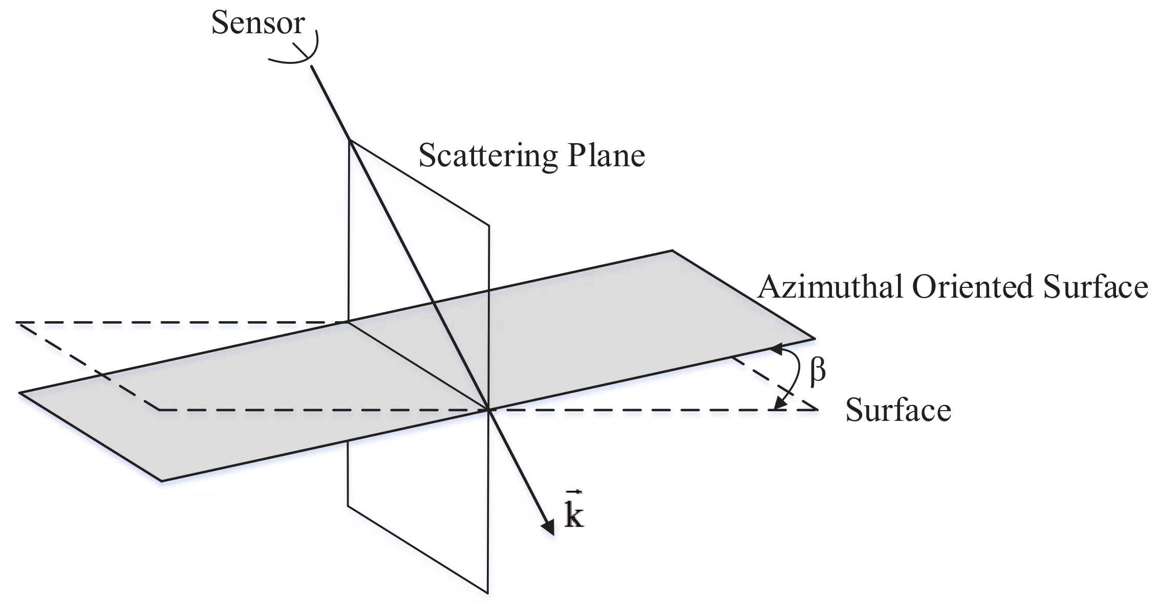
Indeed, Figure 1 shows the corresponding spatial relationship of the surface slope in detail.

The width of the assumed distribution corresponds to the amount of roughness disturbance of the modeled surface [38]. Assuming $P\left(\beta \right)$ to be a uniform distribution about zero with width ${\beta }_1$:

$$P\left(\beta \right)=\left\{\begin{array}{c}\frac{1}{2{\beta }_1}\left|\beta \right|\le {\beta }_1\\ 0\le {\beta }_1\le \frac{\pi }{2}\end{array}.\right.$$

(17)

The coherency matrix for the rough surface becomes:

$$\left[T\right]=\left[\begin{array}{ccc}{T}_{11}& T_{12}& T_{13}\\ T_{21}& T_{22}& T_{23}\\ T_{31}& T_{32}& T_{33}\end{array}\right]=\left[\begin{array}{ccc}{C}_1& C_{2}sinc\left(2{\beta }_1\right)& 0\\ C_{2}sinc\left(2{\beta }_1\right)& C_3(1+sinc\left(4{\beta }_1\right))& 0\\ 0& 0& C_3(1-sinc\left(4{\beta }_1\right))\end{array}\right]$$

(18)

the coefficients $C_1$, $C_2$ and $C_3$ describing the Bragg components of the surface are given by

$$C_1={\sigma }_{HH}^0+{\left({\sigma }_{VV}^0\right)}^2,C_2=({\sigma }_{HH}^0+{\sigma }_{VV}^0)({\left({\sigma }_{HH}^0\right)}^{\ast }-{\left({\sigma }_{VV}^0\right)}^{\ast }),C_3={\left|{\sigma }_{HH}^0-{\sigma }_{VV}^0\right|}^2/2.$$

(19)

For the soil roughness estimation, $ks$ can be calculated by Equation (20)

$$ks=1-A.$$

(20)

With the obtained roughness $ks$, the corresponding entropy H and $\alpha$ angle values are stored in the look-up-table (LUT) by Equations (12) and (14). Using this LUT, the dielectric constant value can be obtained directly from the estimated entropy H and $\alpha$ angle values. Thus, the corresponding moisture $mv$ is obtained.

3. Proposed Parallel Inversion Methods

3.1. Inversion Algorithms Analysis

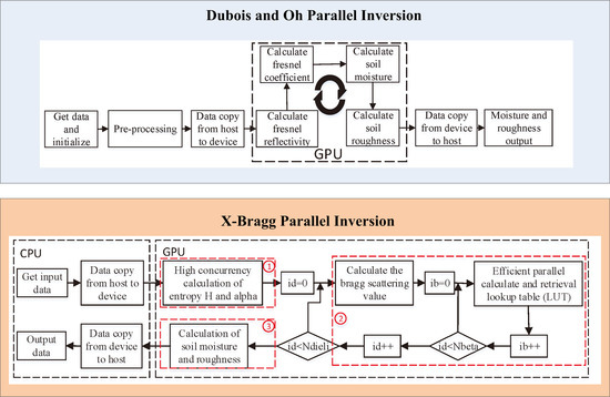
These three inversion algorithms based on Dubois, Oh, and X-Bragg scattering algorithms differ in the aspects of input data, valid ranges, features, and computation complexity, as do the parallel processing methods applied to them, as shown in Figure 2 and Figure 3.

For the inversion of the Dubois algorithm, it is straight and simple from the algorithm equations. At first, the dielectric constant is computed then the surface roughness is calculated. It requires only the scattering coefficients of HH and VV channels, hence they could be applied widely in the presence of the dual pol data availability of many airborne and spaceborne platform. However, it should be noticed that only when the incidence angle is larger than 30 degrees, the algorithm has reliable inversion results. According to Equations (1)–(3), the algorithm complexity is calculated as $O\left(n\right)$, where n indicates the number of PolSAR image pixels. Although the algorithm complexity is ordinary, there are many time-consuming functions including trigonometric and exponential functions, which may reduce the acceleration efficiency.

The Oh algorithm utilizes the full polarimetric scattering coefficients. While for inversion, the Fresnel coefficient is first obtained by an iterative process, following that, the dielectric constant and roughness are computed consequently. Oh has a large valid range of roughness and moisture among the empirical inversion models. When the amplitudes of full polarimetric SAR data are available, it can be applied. According to Equation (4)–(7), its algorithm complexity can be approximated as $O(m·n)$, where m is the number of iterative calculation, and is set to 100 in the experiments. Compared to the Dubois algorithm in computing efficiency, the advantage is that the trigonometric function calculations are avoided, and the disadvantage is that the iterative calculation should be performed.

The X-Bragg algorithm is considered to extend the Bragg scattering algorithm for a slight roughness in the soil surface. It has a wider valid range for the roughness parameter, and is also not sensitive to the existence of slope. The X-Bragg algorithm is the real full polarimetric algorithm for soil surface, which utilizes both the amplitude and the phase information of full polarimetric channels. However, the inversion of this algorithm is not straightforward. The main steps are to compute the roughness from anisotropy, to construct the two-dimensional space of entropy and mean alpha, then to find out the dielectric constant by use of look-up-table (LUT) under certain conditions of incident angle and roughness. According to Equations (8)–(20), the algorithm complexity can be simplified as $d·O(l·n)$, where d indicates the algorithm complexity of matrix diagonalization, l represents the dimension of lookup table. Based on the above complexity analysis, it can be seen that the X-Bragg algorithm is the most complicated calculation, and is worthy of deep optimization.

According to the differences of the three inversion schemes, the key points of parallel computing are thread allocation, data storage, and instruction optimization. For the Dubois and Oh algorithms, two optimization methods were used in our experiment: thread allocation and instruction optimization. For the X-Bragg algorithm, we used a variety of optimization methods such as thread allocation, storage optimization, and instruction optimization.

3.2. GPU-Based Dubois and Oh Parallel Inversion

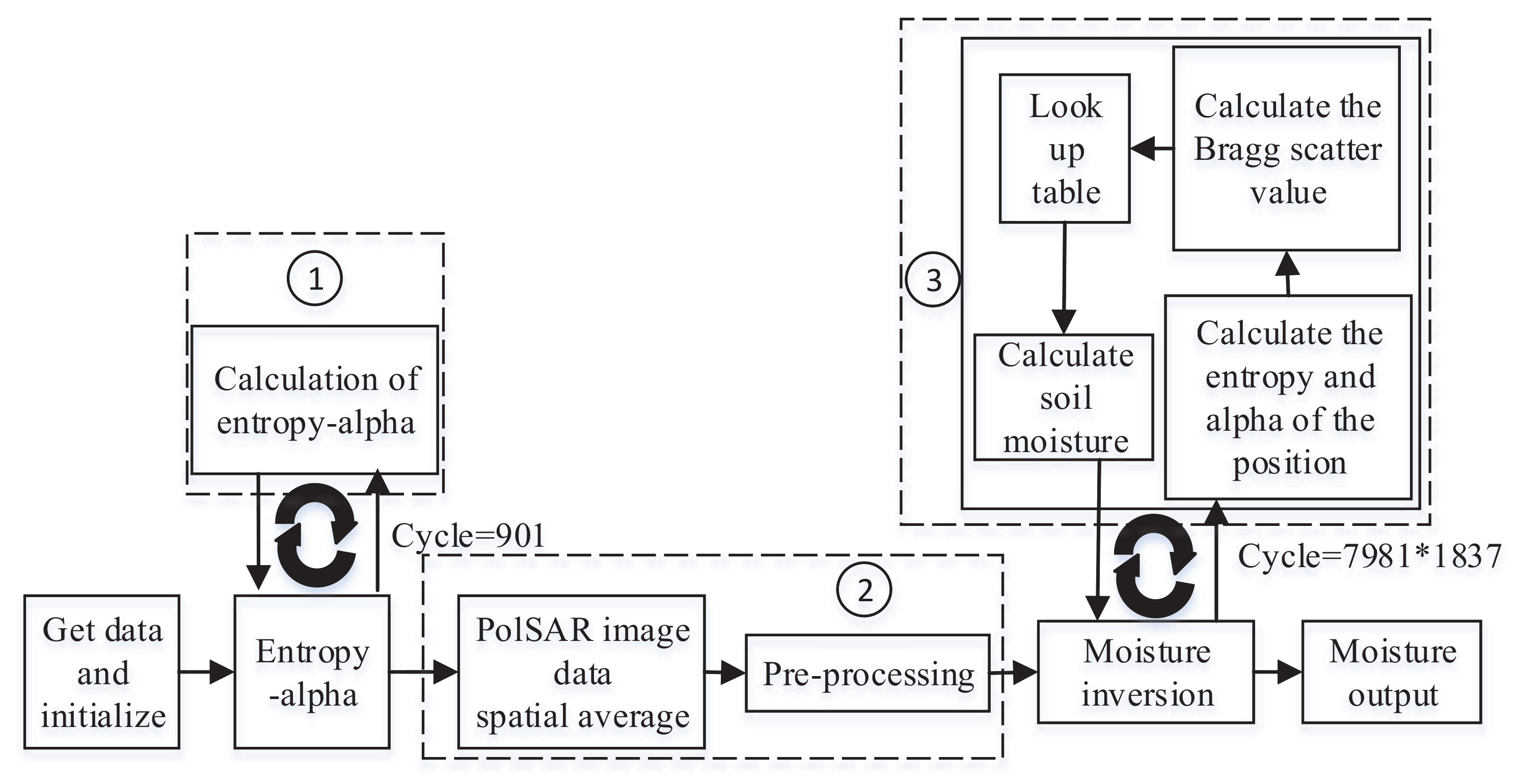
In principle, the Dubois algorithm can be seen as a simplification of the Oh inversion algorithm, so the optimization methods of the two inversion algorithms are roughly the same. The implementation of these two inversion algorithms includes the following parts: data acquisition, data preprocessing, inversion algorithm implementation, and data output. The calculation process of the inversion model is optimized in parallel, which can efficiently achieve the inversion of soil water content and roughness. The overall framework of the inversion algorithm is as follows:

In Figure 2, the black dotted frame is the part that needs to be optimized. The number of cycles of the calculation process is determined by the amount of data. This article uses two ways to optimize:

(1)

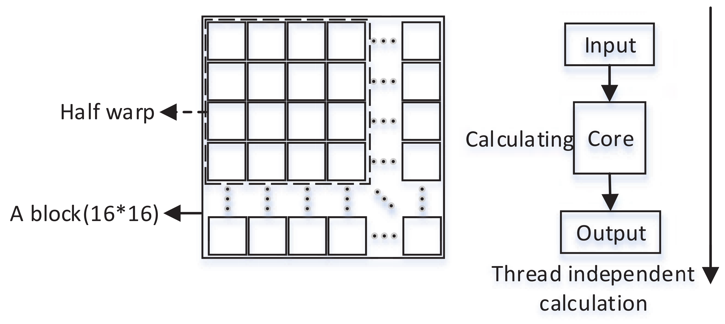
Thread allocation: In the thread allocation process, the computing power of the hardware needs to be considered. In this experimental environment, each block can be allocated up to 1024 threads, which does not mean that the number of threads per block is as high as possible. The amount of data used in the experiment is much larger than 1024, and the pixels remain independent during the calculation, so all threads are independent. Warp is the basic transmission unit of SM (streaming multiprocessor), and a warp has 32 threads. Therefore, the size of each thread block in this experiment is 16 * 16. And the problem of limited storage space for threads is solved. This size ensures the full utilization of each scheduling unit and the threads have sufficient memory. It can make computing more efficient. Figure 3 shows the detailed thread allocation.

(2)

Instruction optimization: In Equations (1), (2), and (7), there are a large number of trigonometric and power functions. When parallel optimization is used, these functions are not applicable. In the CUDA runtime, there are some corresponding mathematical functions, and the calculation efficiency is higher under the condition of partial precision loss. For example, to replace the function sin(.) with the function $\_\_sinf(.)$. The calculation time of the inversion can be reduced by using the $\_\_sinf(.)$ function, which is an internal function of GPU.

3.3. GPU-Based X-Bragg Parallel Inversion

According to the principle of the analytic algorithm, X-Bragg is different from the other two inversion algorithms, and the lookup table is calculated before all data preprocessing. This table is used to find out the corresponding soil moisture under certain conditions of incidence angle and roughness. Figure 4 below shows the overall framework of the inversion algorithm based on X-Bragg.

There are three main parts in the graph. The first one is to calculate the H and $\alpha$ according to X-Bragg algorithm, then H and $\alpha$ are stored in the lookup table. The second part is that the raw data needs to be spatially averaged for preprocessing etc. The third part is the inversion process of X-Bragg algorithm. This part solves the $\left[T\right]$ matrix for each corresponding pixel, and calculates real non-negative eigenvalues ${\lambda }_1$, ${\lambda }_2$, ${\lambda }_3$, and orthogonal eigenvectors ${\overrightarrow{e}}_1$, ${\overrightarrow{e}}_2$, and ${\overrightarrow{e}}_3$. Then the entropy H and $\alpha$ angle are computed corresponding to the eigenvalues and eigenvectors. Following that, the soil roughness can be calculated by scattering anisotropy A ($ks$), and finally with the obtained entropy H and $\alpha$ angle corresponding to the lookup table, soil moisture ($mv$) is inverted.

The size of data used in this experiment was $7981\times 1837$. After testing and averaging six times, the calculation time for each process is obtained. The calculation time of the first part is about 15 ms, and the calculation time of the second and third parts are about 7247 ms and 330,582 ms, respectively. The total computation time is 337,844 ms, in which the third part accounts for 97.85% of the total time. In the local environment, it takes more than five minutes to proceed with data of size $7981\times 1837$, which indicates that X-Bragg algorithm inversion is inefficient and parallelism. Since the third part of the time affects the real-time processing of the inversion, it is considered as the main part for optimization.

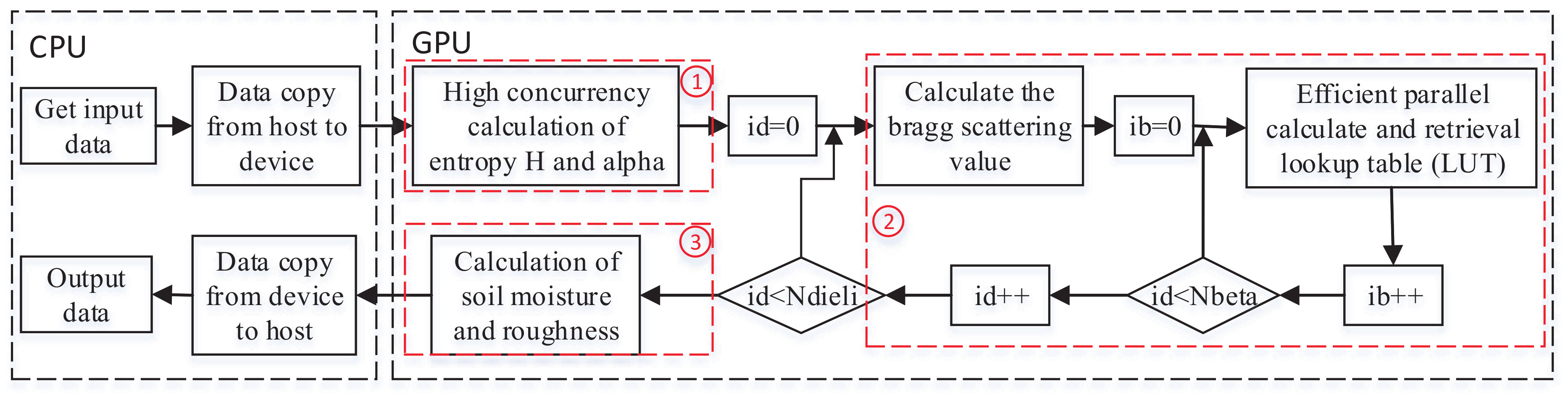
Figure 5 describes in detail the flowchart of CPU/GPU collaborative processing based on inversion algorithms.

In Figure 5, Ndieli is the step size of the inverted dielectric constant. Nbeta is the step size of the roughness angle in the inversion. Through the preliminary test, the display driver stopped responding during the calculation because of the execution time of the kernel function is too long. So the kernel function is divided into three parts: (1) Entropy H and $\alpha$ angle are calculated by high concurrent multithreading; (2) the position of the pixel corresponding to the scatter table is determined, and the entropy H and $\alpha$ angle are calculated using the zero-start consumption of the kernel function; (3) correspond to the lookup table, the moisture ($mv$) and roughness ($ks$) efficiently are calculated.

The pseudo code shows the details of the optimized X-Bragg inversion algorithm.

In pseudo code, the T matrix is calculated. V is the eigenvector and $lambda$ is the corresponding eigenvalue. $al$ and $se$ are calculated as lookup tables. $pos$ is the position in the LUT. $Nlig\ast Ncol$ is the size of the data. $Mmv\_out$ is the output data. In the following part, a detailed optimization analysis of the X-Bragg algorithm is performed through four points.

V1:

Thread allocation optimization

The thread allocation optimization is basically consistent with the analysis of Figure 2. In Figure 4, the experiment is divided into three kernel functions. The first reason is to calculate the time limit. In addition, if the single thread independently calculates the entire inversion process, it will lead to parallel branches. Considering the fact that when the entropy H and $\alpha$ angle are calculated by Equations (17) and (19), there is a threshold judgment $H\le max\_H$ and $\alpha \le max\_\alpha$, while the inversion is only performed in range, so those threads do not perform inversion will be idle. The computation resources is wasted in this way. Therefore, in our experiment the kernel function is split before inversion, which can greatly increase the utilization rate of computing resources and avoid the waste of resources caused by parallel branches.

V2:

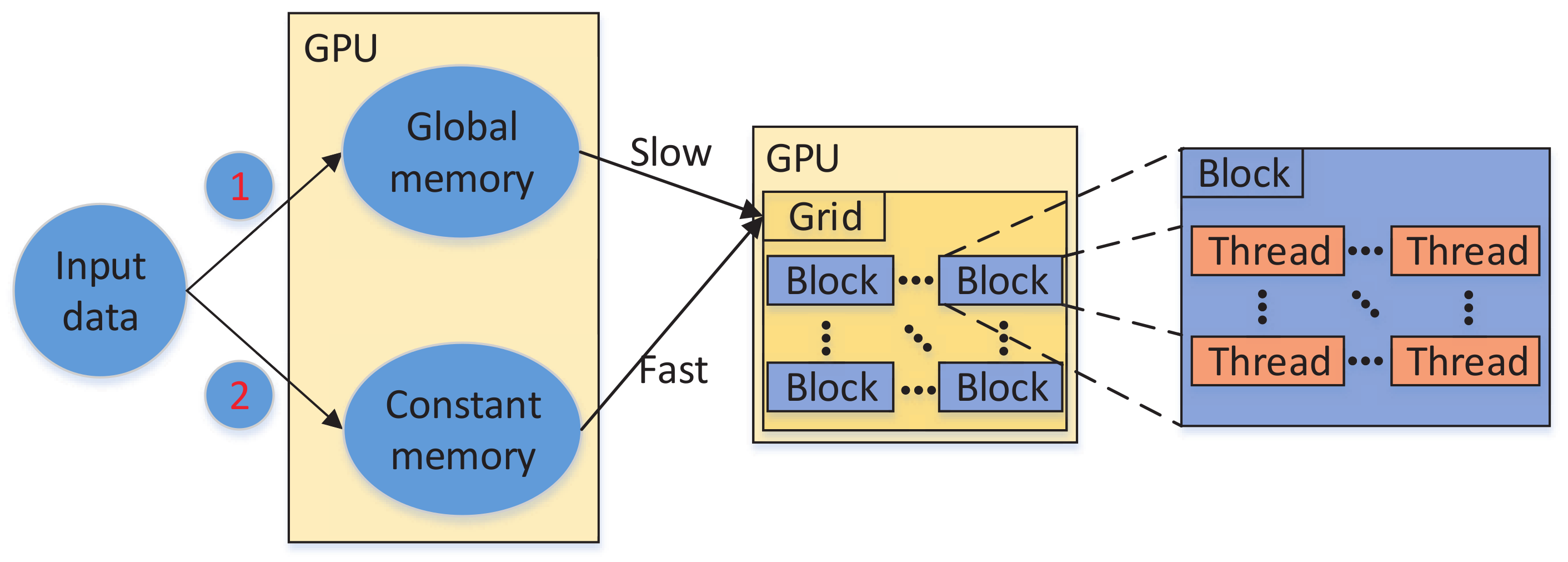
Storage optimization

In the pseudo code, steps 5 and 9 use three constant arrays lia _blockrange, max _en and max _al of size 901. In the process of calculating and searching lookup tables, these three arrays are read multiple times. In general, data is transported from CPU to GPU global memory. Each thread needs to acquire data from the global memory for multiple times, hence the slow transmission time leads to the bottleneck of data processing. This problem can be solved well in hardware storage configuration. Constant memory has 64 kb of storage, and it is much larger than the size of the three arrays. So it is possible to pre-calculate the indices and addresses of the three arrays on CPU and uploaded them to the cached GPU constant memory, where they can be retrieved by the thread blocks at both high bandwidth and low latency. Besides, constant memory is a good fit for these three arrays in read-only operations. In this way, the transmission objective of the data is changed from 1 to 2, as shown in Figure 6.

V3:

Data type conversion optimization

In steps 4 and 8, the diagonalization function is used for multiple times. By implementing Equation (13) $\left[T\right]$ matrix is diagonalized by an unitary similarity transformation, and the non-negative eigenvalue matrix $[\Lambda ]$ and the eigenvector matrix $\left[U_3\right]$ are obtained. This process uses intermediate variables of double-type to make the diagonalization process more precise. But double-type data also limits the speed of GPU operations, while float-type is more suitable than double. Under the AIDA64 software test, the GTX 1080Ti provides a peak throughput of nearly 12.637 teraflop/s in float precision, but is limited to 423 gigaflop/s in double precision. In the GPU, using float data not only reduces memory consumption, but also improves data operation efficiency. Therefore, under the condition of partial accuracy loss, the usage of float-type increases the computational efficiency as well as saving storage resources for the hardware.

V4:

Instruction optimization

In addition to the CUDA fast math optimization mentioned in the other two algorithms, loop expansion is also used for the optimization of the X-Bragg algorithm inversion. In general, a GPU is suitable for processing computationally intensive data, however its ability to do logical judgment is weak. In step 4, step 5, and step 8, the diagonalization process is used multiple times. There are a large number of loops in the process for calculating the real non-negative eigenvalue matrix $[\Lambda ]$ and the eigenvector matrix $\left[U_3\right]$. Logical judgment has also become a huge bottleneck during GPU computing. By artificially expanding the loop within the kernel function, the instruction consumption is reduced as much as possible. Kernel performance is improved to get efficient calculations. In Figure 7, expanding the loop is vividly displayed. GPU is more suitable for computing than CPU. In terms of logical judgment, CPU has higher efficiency.

4. Results

4.1. Experiment Environment

The hardware environment of experimentation includes Intel(R) core(TM) i5-3470 (CPU) and NVIDIA GeForce GTX 1080 Ti (GPU), and the library of visual studio 2013+ CUDA 9.0 is the software environment of the program.

4.2. Accuracy Analysis

Technically, there is no accuracy loss after these algorithms are implemented on GPU. However, there exists a small difference in the accuracy range of CPU and GPU math functions. As for GPU, the computing performance of single-precision floating-point data outperforms double-precision floating-point data by a lot. Therefore, the single-precision floating-point data type is applied for the GPU parallel design. Due to the above two reasons, the proposed methods may bring certain calculation errors, which should be analyzed to guarantee the algorithm accuracy.

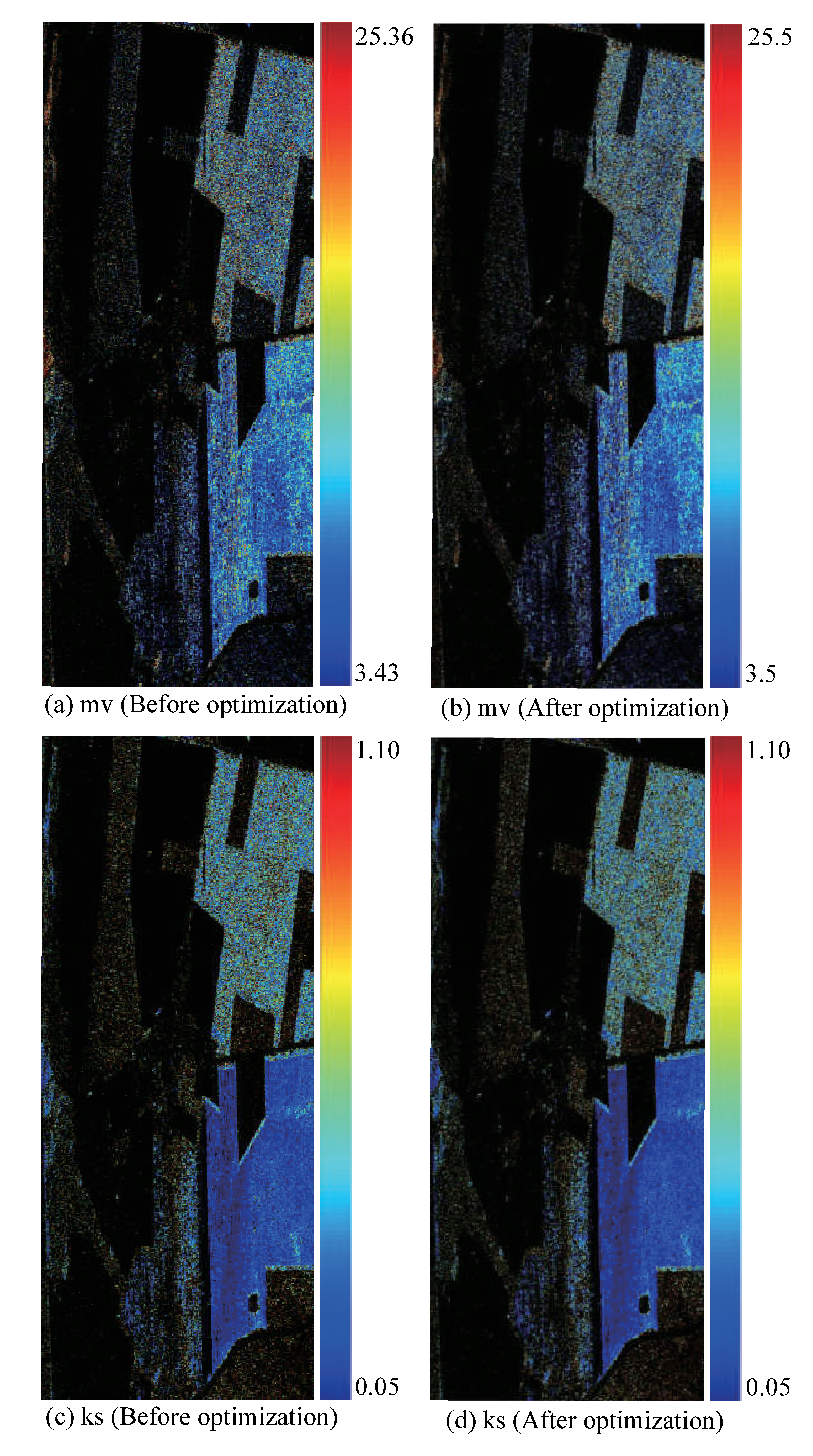
Two indicators are employed to validate the parallel methods, mean absolute error (MAE) and root mean square error (RMSE), respectively. The pixel-wise comparisons of $m_v$ are carried out among the three inversion models, as shown in

Table 1. Calculation error of $m_v$ with CPU and GPU methods.

Model	MAE	RMSE
Dubois	$1.53\times {10}^{-4}$	0.074
Oh	$1.81\times {10}^{-5}$	0.016
X-Bragg	$2.12\times {10}^{-5}$	0.03

. From the MAE and RMSE results, it can be seen that the errors from GPU parallel are very small and can be ignored. Meanwhile, the visual result comparisons on $m_v$ and $k_s$ are shown in Figure 8.

4.3. Optimization Results of the Dubois and Oh Parallel Inversion

The test site is the Demmin area in northern Germany, and the real PolSAR data is acquired by the ESAR airborne system of the German Aerospace Center. The original size is $7981\times 1837$. For comparison, different sizes of data are constructed by the upsampling and downsampling methods. The principle of data construction is to set a size more suitable for each inversion algorithm, which makes the computation more stable. In the above experimental environment, the Dubois and Oh algorithms were tested and compared using the same set of size data. Here, four sizes of data are tested, which are $13600\times 1837$, $6800\times 1837$, $3400\times 1837$, and $1700\times 1837$. After six tests, the average calculation time is used as the final results. Table 1 and

Table 2. Acceleration results of Dubois inversion.

Size	CPU	Running Time (ms)		Speedup
		Calculation	Data Transmission	Calculation	Overall
$\mathrm{13,600}\times 1837$	3814	25	204	$152\times$	$17\times$
$6800\times 1837$	1880	13	101	$144\times$	$16\times$
$3400\times 1837$	839	6	51	$139\times$	$15\times$
$1700\times 1837$	424	2	27	$212\times$	$14\times$

below show the calculation time for Dubois and Oh algorithms at different data sizes.

In Table 2 and

Table 3. Acceleration results of Oh inversion.

Size	CPU	Running Time (ms)		Speedup
		Calculation	Data Transmission	Calculation	Overall
$\mathrm{13,600}\times 1837$	32,698	27	298	$1211\times$	$100\times$
$6800\times 1837$	15,453	13	149	$1188\times$	$95\times$
$3400\times 1837$	6633	7	74	$947\times$	$82\times$
$1700\times 1837$	3361	2	35	$1680\times$	$90\times$

, the row data represents the calculation time for different sizes. The first column indicates CPU computation time. The second column shows the transmission time of all data from CPU to GPU. The third column is the computation time of the kernel function. The fourth column shows the overall speedup results of the inversion based on the scattering algorithm.

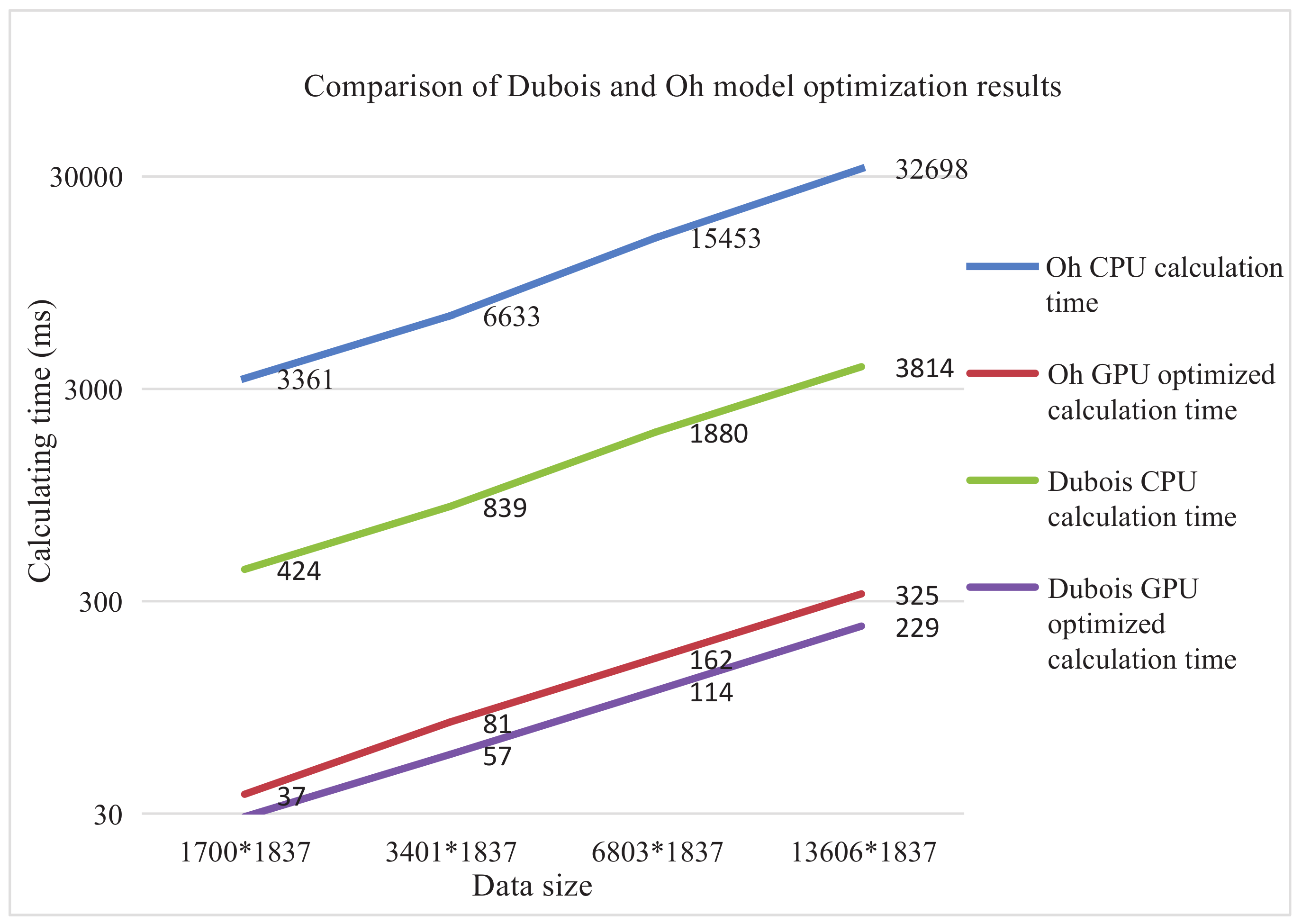
Table 2 shows the optimization results of the Dubois model inversion. The performance of the GPU has only increased by about 15 times. As the amount of data decreases, the speedup effect is gradually weakened. This further illustrates pertinence of GPU for computationally intensive data. The acceleration can reach hundreds of times without considering the data transmission time. In Table 3, GPU is 100 times faster than CPU. Here, the computation time can be accelerated by thousands of times without considering the data transmission.

In terms of algorithm, Oh is more complicated than Dubois. In CPU calculation process, Oh is much slower than Dubois. This shows that the complexity of the calculation process has a profound impact on GPU usage. From the two algorithms optimization results, Oh is more suitable for GPU than Dubois. The Figure 9 is a more intuitive description of the optimization of these two algorithms.

4.4. Optimization Result of the X-Bragg Parallel Inversion

In the above experimental environment, The $15862\times 1837$, $7981\times 1837$, $3990\times 1837$, and $1995\times 1837$ size data were used in the X-Bragg algorithm.

Table 4. Acceleration results of the X-Bragg inversion.

Size	CPU	Running Time (ms)		Speedup
		Final Calculation	Data Transmission	Calculation	Overall
$\mathrm{15,862}\times 1837$	66,0481	3808	368	173×	158×
$7981\times 1837$	330,508	1911	194	172×	157×
$3990\times 1837$	165,441	1250	97	132×	122×
$1995\times 1837$	82,813	441	48	187×	169×

details the calculation time of the algorithm in different situations.

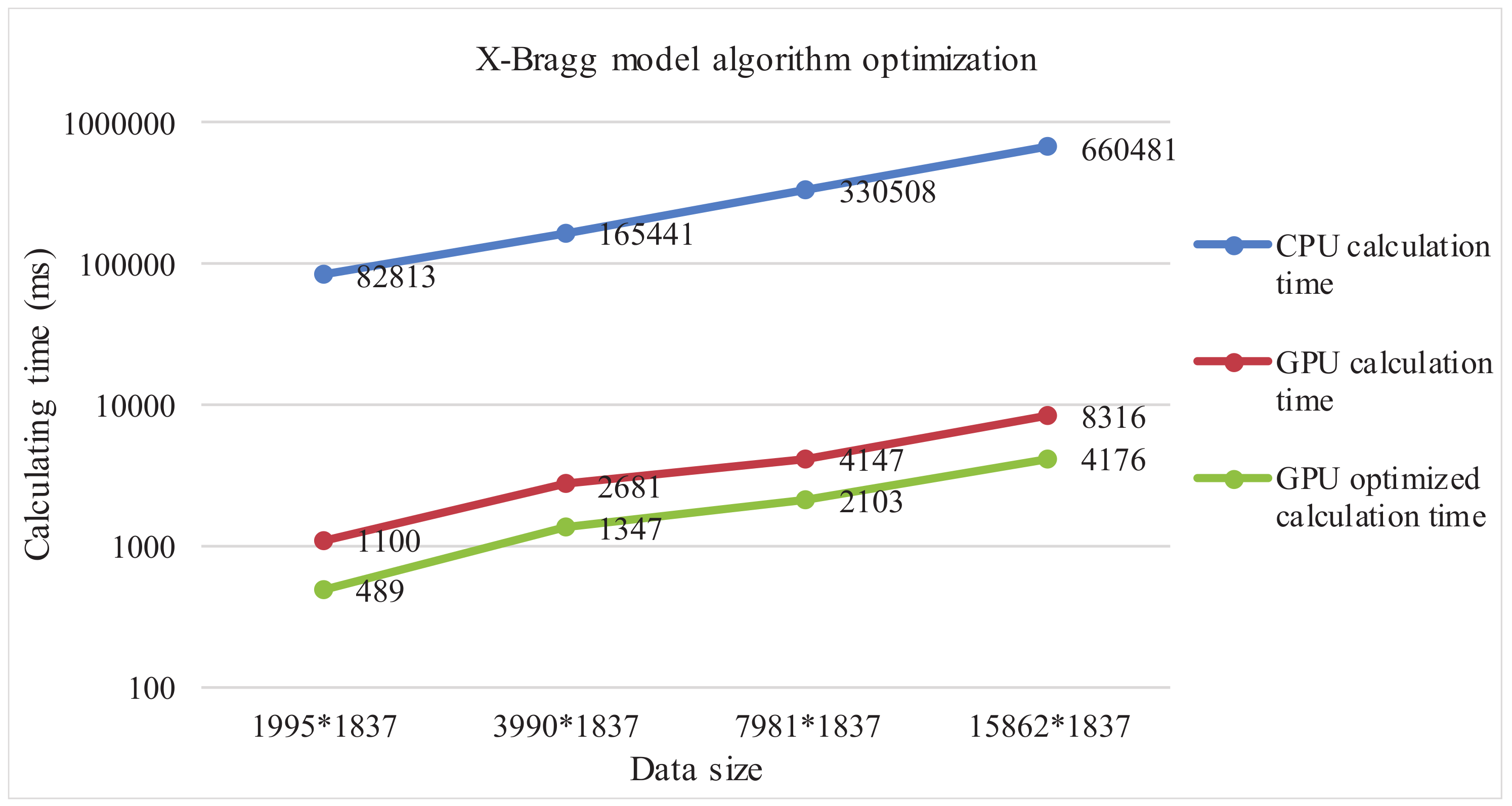
In Table 4, CPU time is the time before optimization. The final computation time is the one after the final optimization. As can be seen from the table, the final result is about 150 times faster than CPU. In Figure 10, the acceleration effects of different data sizes can be clearly expressed.

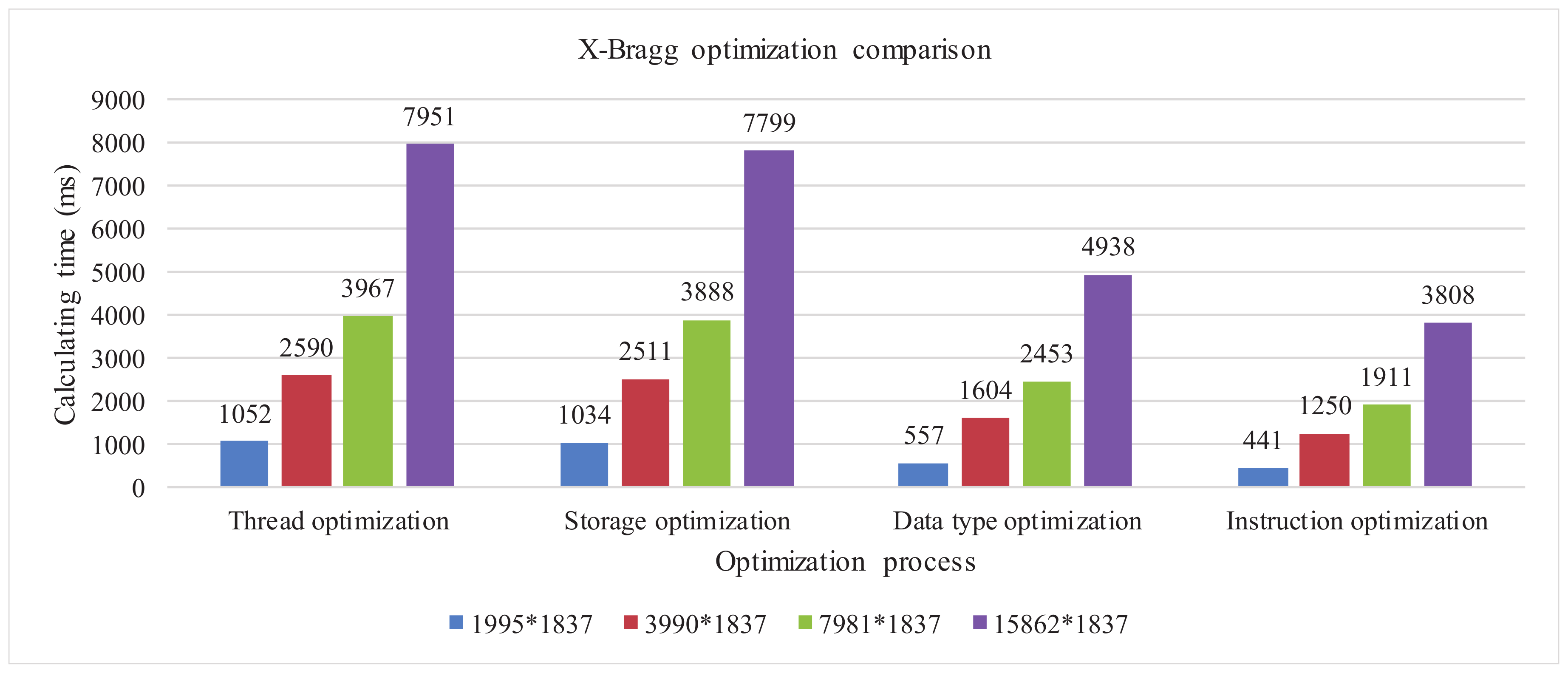
This experiment proposes four optimization methods based on the complexity of the algorithm. They are thread allocation, storage optimization, data conversion, and instruction optimization, respectively.

Table 5. Calculation time (ms) of the X-Bragg inversion after different optimization steps.

Size	V1	V2	V3	V4
$\mathrm{15,862}\times 1837$	7951	7799	4938	3808
$7981\times 1837$	3967	3888	2453	1911
$3990\times 1837$	2590	2511	1604	1250
$1995\times 1837$	1052	1034	557	441

shows the time tested after each step optimization.

In Table 5, the first column is the optimization result after reasonable thread allocation for hardware. The second column shows the effect after using constant memory. The third column shows the time after type conversion optimization. The fourth column is the final optimization result after the loop is expanded. From the first column to the fourth column optimization, the efficiency of the process is more than doubled. The acceleration performances of X-Bragg algorithm at different data size with different optimization methods are also shown in Figure 11.

In Figure 11, bar graphs of different colors represent data of different sizes. With the implementation of the four optimization methods, the calculation time is continuously reduced. The number on the graph indicates the detailed calculation time (unit: ms). On the whole, the final optimization can reach more than $150\times$ speedup. Taking $15862\times 1837$ data as an example, the inversion time is reduced from 11 min to 4 s.

5. Conclusions

In this paper, three classical forward scattering models and their corresponding inversion algorithms are analyzed. They are different in polarimetric data requirement, application situation, and performance. Through the further analysis of the structure of the three classical inversion algorithms based on scattering models, each algorithm is optimized, respectively. Then a framework for the parallel inversion method for polarimetric SAR imagery based on GPU is presented. The optimization combines the processing advantages of a GPU with computationally intensive imagery, so as to realize the parallel design of three inversion algorithms, including the entire inversion process from data transmission, computational instruction set, to GPU hardware structure. In the experiments, the calculation efficiency is increased by approximately 100-fold. For all widely used empirical models, the problems of large data volume and low computing efficiency are solved, including dual/multi/full polarization models. Experiments with real data fully demonstrate the tremendous advantages of combining GPU and PolSAR imagery for real-time processing. However, as far as the calculation time is concerned, the parallel X-Bragg method is still two orders of magnitude slower than the other two methods. In the future work, we will further optimize the diagonalization part to make it more efficient.

References

- Du, C.; Qin, Q.; Liu, M.; Feng, H.; Dong, H.; Wang, N. Soil moisture inversion and validation based on new remote sensing platform. In Proceedings of the IEEE International Geoscience and Remote Sensing Symposium, Melbourne, Australia, 21 July 2013; pp. 2728–2731. [Google Scholar]
- Kweon, S.K.; Oh, Y. Estimation of soil moisture and surface roughness from single-polarized radar data for bare soil surface and comparison with dual-and quad-polarization cases. IEEE Trans. Geosci. Remote Sens. 2013, 52, 4056–4064. [Google Scholar] [CrossRef]
- Verstraeten, W.; Veroustraete, F.; Feyen, J. Assessment of evapotranspiration and soil moisture content across different scales of observation. Sensors 2008, 8, 70–117. [Google Scholar] [CrossRef] [PubMed] [Green Version]
- Yin, Q.; Cao, F.; Hong, W. Analysis of Valid Ranges in Soil Inversion Models Based on the Cloude-Pottier Decomposition. In Proceedings of the IEEE International Geoscience and Remote Sensing Symposium, Boston, MA, USA, 7–11 July 2008; pp. II-821–II-823. [Google Scholar]
- Dobriyal, P.; Qureshi, A.; Badola, R.; Hussain, S.A. A review of the methods available for estimating soil moisture and its implications for water resource management. J. Hydrol. 2012, 458, 110–117. [Google Scholar] [CrossRef]
- Jiao, J.; Zhang, Y.; Sun, H.; Yang, X.; Gao, X.; Hong, W.; Fu, K.; Sun, X. A Densely Connected End-to-End Neural Network for Multiscale and Multiscene SAR Ship Detection. IEEE Access 2018, 6, 20881–20892. [Google Scholar] [CrossRef]
- Li, H.; Krylov, V.; Fan, P.; Zerubia, J.; Emery, W. Unsupervised Learning of Generalized Gamma Mixture Model with Application in Statistical Modeling of High- Resolution SAR Images. IEEE Transac. Geosci. Remote Sens. 2016, 54, 2153–2170. [Google Scholar] [CrossRef] [Green Version]
- Chen, H.; Zhang, F.; Tang, B.; Yin, Q.; Sun, X. Slim and efficient neural network design for resource-constrained SAR target recognition. Remote Sens. 2018, 10, 1618. [Google Scholar] [CrossRef] [Green Version]
- Gao, F.; Xue, X.; Sun, J.; Wang, J.; Zhang, Y. A SAR image despeckling method based on two-dimensional S-transform shrinkage. IEEE Trans. Geosci. Remote Sens. 2016, 54, 3025–3034. [Google Scholar] [CrossRef]
- Gao, F.; Yang, Y.; Wang, J.; Sun, J.; Yang, E.; Zhou, H. A Deep Convolutional Generative Adversarial Networks (DCGANs)-Based Semi-Supervised Method for Object Recognition in Synthetic Aperture Radar (SAR) Images. Remote Sens. 2018, 10, 846. [Google Scholar] [CrossRef] [Green Version]
- Srivastava, P.K.; Pandey, P.C.; Petropoulos, G.P.; Kourgialas, N.N.; Pandey, V.; Singh, U. GIS and Remote Sensing Aided Information for Soil Moisture Estimation: A Comparative Study of Interpolation Techniques. Resources 2019, 8, 70. [Google Scholar] [CrossRef] [Green Version]
- Piles, M.; Petropoulos, G.P.; Sanchez, N.; Gonzalez-Zamora, A.; Ireland, G. Towards improved spatio-temporal resolution soil moisture retrievals from the synergy of SMOS and MSG SEVIRI spaceborne observations. Remote Sens. Environ. 2016, 180, 403–417. [Google Scholar] [CrossRef] [Green Version]
- Yin, Q.; Hong, W.; Zhang, F.; Pottier, E. Optimal Combination of Polarimetric Features for Vegetation Classification in PolSAR Image. IEEE J. Sel. Top. Appl. Earth Observ. Remote Sens. 2019, 12, 3919–3931. [Google Scholar] [CrossRef]
- Zhang, F.; Hu, C.; Li, W.; Hu, W.; Li, H. Accelerating Time-Domain SAR Raw Data Simulation for Large Areas Using Multi-GPUs. IEEE J. Sel. Top. Appl. Earth Obs. Remote Sens. 2014, 7, 3956–3966. [Google Scholar] [CrossRef]
- Jung, S.G.; Hong, J.Y.; Oh, Y. Verification of Surface Scattering Models and Inversion Algorithms with the Polarimetric Backscatter Measurements of a Bare Soil Surface. In Proceedings of the Asia-Pacific Microwave Conference, Bangkok, Thailand, 11 December 2007; pp. 1–3. [Google Scholar]
- Qiu, C.; Chen, Y.; Tong, L.; Jia, M.; Pang, S. The method for soil moisture inversion based on ground-based scattering measurement. In Proceedings of the IEEE International Geoscience and Remote Sensing Symposium, Vancouver, BC, Canada, 24 July 2011; pp. 3086–3088. [Google Scholar]
- Kweon, S.K.; Park, S.M.; Oh, Y. Improvement of soil moisture inversion for single-polarized SAR data of bare soil surfaces using DInSAR technique. In Proceedings of the IEEE Geoscience and Remote Sensing Symposium, Quebec City, QC, Canada, 13 July 2014; pp. 3236–3238. [Google Scholar]
- Xue, Q.; Sheng, Q.; Ma, S. Application of Optimum Perturbation Algorithm for Parameter Inversion Identification of Soil Moisture Model under Ecological Slope Protection. In Proceedings of the IEEE International Conference on Artificial Intelligence and Computational Intelligence, Shanghai, China, 7 November 2009; Volume 1, pp. 204–207. [Google Scholar]
- Wang, Y.; Li, Y.; Sun, S.; Zhou, Q.; Han, N. Research on inversion of soil water dynamic parameters by field soil moisture content. In Proceedings of the IEEE International Conference on New Technology of Agricultural, Zibo, China, 27 May 2011; pp. 338–343. [Google Scholar]
- Oh, Y.; Jung, S.G. Inversion Algorithm for Soil Moisture Retrieval from Polarimetric Backscattering Coefficients of Vegetation Canopies. In Proceedings of the IEEE International Geoscience and Remote Sensing Symposium, Boston, MA, USA, 7 July 2008; Volume 2, pp. II-402–II-405. [Google Scholar]
- Oh, Y. Comparison of two inversion methods for retrieval of soil moisture and surface roughness from polarimetric radar observation of soil surfaces. In Proceedings of the IEEE International Geoscience and Remote Sensing Symposium, Anchorage, AL, USA, 20 September 2004; Volume 2, pp. 807–810. [Google Scholar]
- Geddert, N.; Jeffrey, I. A Dynamically Balanced OpenMP-CUDA Implementation of PDE-Based Contrast Source Inversion for Microwave Imaging. In Proceedings of the International Symposium on Antenna Technology and Applied Electromagnetics, Waterloo, ON, Canada, 19 August 2018; pp. 1–2. [Google Scholar]
- Li, M.; Wang, X.Y.; Abubakar, A. Accelerating nonlinear inversion algorithms on GPU platform for electromagnetic data. In Proceedings of the International Symposium on Antennas and Propagation, Okinawa, Japan, 24 October 2016; pp. 574–575. [Google Scholar]
- Wang, X.Y.; Li, M.; Abubakar, A. Acceleration of multiplicative regularized contrast source inversion algorithm using paralleled computing architecture. In Proceedings of the IEEE Progress in Electromagnetic Research Symposium, Shanghai, China, 8 August 2016; pp. 1739–1743. [Google Scholar]
- Ries, F.; De Marco, T.; Zivieri, M.; Guerrieri, R. Triangular matrix inversion on graphics processing unit. In Proceedings of the ACM Conference on High Performance Computing Networking, Storage and Analysis, Portland, OR, USA, 14 November 2009; pp. 1–10. [Google Scholar]
- Gao, C.; Li, L.; Zhao, Z.; Huang, H. Parallel computation of the large grounding grids in multi-layer soil using moment method. In Proceedings of the IEEE World Automation Congress, Hawaii, HI, USA, 28 September 2008; pp. 1–4. [Google Scholar]
- Gomez-Calvino, J.; Colominas, I.; Navarrina, F.; Casteleiro, M.; Cela, J. Parallel computing aided design of earthing systems for electrical substations in non-homogeneous soil models. In Proceedings of the IEEE International Workshop on Parallel Processing, Toronto, ON, Canada, 21 August 2000; pp. 381–388. [Google Scholar]
- Zhang, F.; Hu, C.; Wu, P.; Zhang, H.; Wong, M. Accelerating aerial image simulation using improved CPU/GPU collaborative computing. Comput. Electr. Eng. 2015, 46, 176–189. [Google Scholar] [CrossRef]
- Hu, C.; Zhang, F.; Li, G.; Li, W.; Cui, Z. Computation Reduction Oriented Circular Scanning SAR Raw Data Simulation on Multi-GPUs. J. Radars 2016, 5, 434–443. [Google Scholar]
- Li, Z.; Su, D.; Zhu, H.; Li, W.; Zhang, F.; Li, R. A Fast Synthetic Aperture Radar Raw Data Simulation using Cloud Computing. Sensors 2017, 17, 113. [Google Scholar] [CrossRef] [PubMed] [Green Version]
- Tang, H.; Li, G.; Zhang, F.; Hu, W.; Li, W. A spaceborne SAR on-board processing simulator using mobile GPU. In Proceedings of the IEEE International Geoscience and Remote Sensing Symposium, Beijing, China, 10 July 2016; pp. 1198–1201. [Google Scholar]
- Zhang, F.; Hu, C.; Li, W. A deep collaborative computing based SAR raw data simulation on multiple CPU/GPU platform. IEEE J. Sel. Top. Appl. Earth Obs. Remote Sens. 2016, 10, 387–399. [Google Scholar] [CrossRef]
- Zhang, F.; Yao, X.; Tang, H.; Yin, Q.; Hu, Y.; Lei, B. Multiple mode SAR raw data simulation and parallel acceleration for gaofen-3 mission. IEEE J. Sel. Top. Appl. Earth Obs. Remote Sens. 2018, 11, 2115–2126. [Google Scholar] [CrossRef]
- Li, G.; Zhang, F.; Ma, L.; Hu, W.; Li, W. Accelerating SAR imaging using vector extension on multi-core SIMD CPU. In Proceedings of the IEEE International Geoscience and Remote Sensing Symposium, Milan, Italy, 26 July 2015; pp. 537–540. [Google Scholar]
- Hu, C.; Zhang, F.; Ma, L.; Li, G.; Hu, W.; Li, W. Efficient SAR raw data parallel simulation based on multicore vector extension. In Proceedings of the IEEE International Geoscience and Remote Sensing Symposium, Milan, Italy, 26 July 2015; pp. 4719–4722. [Google Scholar]
- Oh, Y.; Sarabandi, K.; Ulaby, F.T. An empirical model and an inversion technique for radar scattering from bare soil surfaces. IEEE Trans. Geosci. Remote Sens. 1992, 30, 370–381. [Google Scholar] [CrossRef]
- Smith, J.R.; Mirotznik, M.S. Rough surface scattering models. In Proceedings of the IEEE International Geoscience and Remote Sensing Symposium, Anchorage, AL, USA, 20 September 2004; Volume 5, pp. 3107–3110. [Google Scholar]
- Hajnsek, I.; Pottier, E.; Cloude, S.R. Inversion of surface parameters from polarimetric SAR. IEEE Trans. Geosci. Remote Sens. 2003, 41, 727–744. [Google Scholar] [CrossRef]
Figure 1.
Surface slope diagram.
Figure 2.
Dubois and Oh inversion algorithm optimization framework.
Figure 3.
Thread allocation strategy.
Figure 4.
X-Bragg algorithm framework.
Figure 5.
Optimization flowchart of the X-Bragg algorithm.
Figure 6.
Storage optimization strategy.
Figure 7.
Loop unfolding optimization strategy.
Figure 8.
The soil parameter inversion comparison of sequential and parallel optimization Oh methods.
Figure 9.
Comparison of the Dubois and Oh algorithm optimization results.
Figure 10.
Acceleration performance comparison of the X-Bragg algorithm.
Figure 11.
Results of using different optimization methods.