Time Series Remote Sensing Data-Based Identification of the Dominant Factor for Inland Lake Surface Area Change: Anthropogenic Activities or Natural Events?

Abstract

Inland lake variations are considered sensitive indicators of global climate change. However, human activity is playing as a more and more important role in inland lake area variations. Therefore, it is critical to identify whether anthropogenic activity or natural events is the dominant factor in inland lake surface area change. In this study, we proposed a method that combines the Douglas-Peucker simplification algorithm and the bend simplification algorithm to locate major lake surface area disturbances. These disturbances were used to extract the features that been used to classify disturbances into anthropogenic or natural. We took the nine lakes in Yunnan Province as test sites, a 31-year long (from 1987 to 2017) time series Landsat TM/OLI images and HJ-1A/1B used as data sources, the official records were used as references to aid the feature extraction and disturbance identification accuracy assessment. Results of our method for disturbance location and disturbance identification could be concluded as follows: (1) The method can accurately locate the main lake changing events based on the time series lake surface area curve. The accuracy of this model for segmenting the time series of lake surface area in our study area was 94.73%. (2) Our proposed method achieved an overall accuracy of 87.75%, with an F-score of 85.71 for anthropogenic disturbances and an F-score of 88.89 for natural disturbances. (3) According to our results, lakes in Yunnan Province of China have undergone intensive disturbances. Human-induced disturbances occurred almost twice as much as natural disturbances, indicating intensified disturbances caused by human activities. This inland lake area disturbance identification method is expected to uncover whether a disturbance to inland lake area is human activity-induced or a natural event, and to monitor whether disturbances of lake surface area are intensified for a region.

1. Introduction

Inland lakes are important aspects of land surface cover that participate in the natural water cycle and are considered highly sensitive to the impacts of climate change and human activities [1,2]. Shrinkage or extension of inland lakes can reflect global climate and environment changes [3]. Thus, inland lake variations are considered sensitive indicators of global climate change [4,5]. Lake variations are caused by either natural events or anthropogenic activities. However, these variations are mostly documented by the local authorities or institutions and are rarely obtained from remote sensing technology.

This study focuses on remote sensing methods to identify the dominant factors affecting changes to inland lake surface area. With advantages of wide coverage, high frequency data collection, labor and economic cost-effectiveness, remote sensing technology has been used in previous lake change studies [6,7,8], especially for lakes located in remote and less developed areas where lake surface changes have been only rarely documented [2].

With ongoing earth observation projects (such as NASA’s Earth Observing System (EOS) and the European Union’s Copernicus program) and the development of sensors (from visible to infrared and SAR), time series of remote sensing data is providing a new means to study lake change. Remote sensing data used for lake monitoring could be divided into three categories according to their spatial resolution: coarse-, medium- and high-spatial resolution data. Although coarse spatial resolution remote sensing data (such as NOAA/AVHRR, MODIS, Suomi NPP-VIIRS and Sentinel-3) have lower spatial resolution and larger FOV (Field of View) that cause BRDF (bidirectional reflectance distribution function) effects [9], they often have a higher revisit frequency and a wider coverage; therefore, they have been widely used in water monitoring [10]. For example, Feng et al. [11] quantified the effect of seven potential driving factors (from both human activities and natural processes) in 50 large lakes on the Yangtze Plain using time series of MODIS observations between 2003 and 2016; they found human activities significantly influenced more lakes than natural processes in this area. Che et al. [12] applied the synthesized monthly MODIS09A1 data to extract the lake area of the Qinghai-Tibet Plateau from 2000 to 2013 using the synthesized normalized difference water index (NDWI) of a water body index proposed by Mcfeeters [13]. Their results showed that the lake area of the Qinghai-Tibet Plateau significantly expanded during 2000 and 2013. Using time series MODIS data to identify Poyang lake water area changes, Feng et al. [14] found that Poyang Lake had significant seasonal and interannual changes during 2000 and 2010, mainly due to the influence of climate fluctuations. With the development of better sensors, high spatial resolution land monitoring satellites, such as QuickBird, IKONOS, Worldview, RapidEye, ZY-3 and GF-1/2, can provide more accurate and higher spatially resolved land cover observations. However, the small image coverage and the long revisit periods of high spatial resolution data remain obstacles for the detection of change in larger inland water bodies [6].

Among these three kinds of data, the medium-resolution data, such as Landsat, HJ-1A/B, ASTER and Sentinel-2 data, are the most widely used in water monitoring applications. The main reason for their frequency of use is the free data access policy and the long-term monitoring of Earth’s surface changes that these datasets represent, e.g., Landsat data includes continuous observations of up to 48 years [15,16,17]. A wide range of studies have been employed to study changes to the lake surfaces using medium-resolution remote sensing data. For example, in order to obtain the water area of the Yunnan-Guizhou Plateau from 1985 to 2015, Xiao et al. [18] extracted lake surface areas using Landsat image data from five periods at an interval of 5 years and found that the water area of lakes in the Yunnan-Guizhou Plateau first increased and then decreased during this period. Tulbure et al. [8] studied the relationship between water body areas and changes in the weather in the Murray-Darling Basin and the Barmah-Millewa forests from 1986 to 2011; the results show that extreme weather events, such as drought and rainfall, have a significant impact on surface water bodies and submergence dynamics. Using Landsat time series data, Arvor et al. [19] developed a method for automatically identifying small water bodies and used it to extract the area and quantity of small reservoirs in the Amazon region of southern Brazil from 1985 to 2015. The results show that the total area and quantity of small reservoirs in the area increased by 10 times and more than five times during the study period, respectively.

In summary, existing remote sensing technology used in inland water body identification with median spatial resolution has provided reliable results for monitoring inland lake change. Moreover, current studies are focusing on quantifying the lake water quality that contributed by human activities or natural processes [10], or how surface water is altered by human activities [2]. For inland lake area change, we need to further know where and when a major inland surface water area disturbance occurred, and whether this lake surface area change dominated by human activities or natural events. This identification is critical for uncovering the relationship between human activities and the natural environment on both local and global scales. Thus, in this study, we take nine large inland lakes on the Yunnan Plateau of southwest China as our study area and apply the proposed lake surface area change analysis method to uncover changes in inland lakes and to identify whether human activities or natural events dominate these changes.

2. Study Area and Data

2.1. Overview of Study Area

The Yunnan Plateau is part of the Yunnan-Guizhou Plateau, which is one of the four major plateaus in China. This area is located in southwest China and is characterized by rough terrain and a subtropical monsoon climate. There are many inland lakes on the Yunnan-Guizhou Plateau; lakes here play important roles in the ecological environment and regional water security and have even been considered important strategic resources for the state economy and social development.

There are more than 40 lakes that vary in size on the Yunnan Plateau and lake basins are where industry and agriculture activities are mostly concentrated. The nine lakes selected for this study are located in different areas with varied geographical environments in Yunnan Province (Figure 1) and include five faulted tectonic lakes (Dianchi Lake, Qilu Lake, Erhai Lake, Haixi Lake and Bita Lake), one faulted karst lake (Lashi Lake), one structural faulted glacial lake (Shudu Lake) located in northwest Yunnan and two karst lakes (Yilong Lake and Yuxian Lake) located in south and southeast Yunnan. The nine lakes span the tropical monsoon climate zone and the subtropical monsoon climate zone with dry winters. There are typically two seasons under these climate zones, the dry season (from November to the next April) and the rainy season (from May to October of a year). This climate condition is critical for the optical remote sensing of lakes in this area. The elevation of Yunnan Province varies from 1420 m a.s.l. (metres above sea level) to 3620 m a.s.l. Among the nine lakes, Dianchi Lake, known as the “Plateau Pearl,” is the largest freshwater lake in Yunnan Province; Yuxian Lake completely dried out in several years according to surveys by Li et al. [20]. The surface area of this lake rapidly decreased to approximately only 150 m² in August 2013 and the lake had completely dried up when a survey was conducted again in March 2014 by Hu Kui. Qilu Lake and Yilong Lake are undergoing severe anthropogenic disturbance, and Bita Lake is currently being subjected to minimal anthropogenic disturbance. These lakes are distributed in different regions and at different elevations and are therefore highly representative.

2.2. Data Source and Preprocessing

In this study, Landsat TM/OLI remote sensing image data with a time span of 31 years (1987–2017) were used as the main data source for extracting lake surface area. There were no high-quality Landsat data available between November 3, 2011 and April 12, 2013 for this study area except SLC-off (Scanning Line Corrector off) ETM+ images. Therefore, we used HJ-1A/B CCD data, which has the same spatial resolution as the Landsat data (30 m spatial resolution), to supplement the missing Landsat data during this period. The level-1 Landsat data were downloaded from the United States Geological Survey website (https://glovis.usgs.gov/) and the HJ-1A/B data were downloaded from the China Centre for Resources Satellite Data and Application (CRESDA) (http://www.cresda.com/). Because of the distinct dry and wet seasons in Yunnan Province, approximately 90% of the year’s precipitation is concentrated in the rainy season, while only 10% occurs during the dry season [21]. As a consequence, available remote sensing images for the rainy season in this study area are very limited. Remote sensing images we used in this study were all selected during the dry season to ensure that there would be at least one available Landsat observation for each year. We finally downloaded 795 Landsat level-1 images (see

Table 1. Remote sensing images used in this study.

Date	Satellite Sensors	Images Selected	Spatial Resolution	Data Source
11/01/1986-11/02/2011	Landsat TM	686	30 m	https://glovis.usgs.gov/
11/03/2011-04/12/2013	HJ-1A/B	27	30 m	http://www.cresda.com/
04/13/2013-04/30/2017	Landsat OLI	109	30 m	https://glovis.usgs.gov/

for details). In addition, we selected 27 cloud-free HJ-1A/B images covering the nine lakes in the study area between November 3, 2011 and April 12, 2013.

Remote sensing data used in this study were preprocessed, which included radiation calibration, atmospheric correction and geometric correction. For the atmosphere correction of Landsat data, the FLAASH (Fast Line-of-sight Atmospheric Analysis of Spectral Hypercubes) model, which is based on the ModTRAN model on ENVITM 5.3 software, was used to create the Landsat-based surface reflectance data [22]. Because clouds and cloud shadows are obstacles to classification tasks using visible spectral remote sensing techniques, the Fmask algorithm provided by Zhu was used to identify the clouded and shadowed pixels [23], and these identified pixels were removed and filled with the nearest available data. The radiation calibration and atmospheric correction of the HJ-1A/B data were also performed using ENVITM 5.3 software. The calibration parameters and spectral response functions required for the radiation calibration and the atmospheric correction of the HJ1A/B data were obtained from the China Centre for Resources Satellite Data and Application CRESDA website (http://www.cresda.cn/CN/Downloads/dbcs/index.shtml). To keep the consistency between Landsat and HJ-1A/B data derived lake surface areas, Landsat orthophoto images were used as reference images to register the HJ-1A/B data, and approximately 16 ground control points (GCPs) were uniformly selected for each image. These GCPs were used in coregistration between Landsat and HJ-1A/B CCD data applying polynomial model and the nearest neighbor resampling method.

The water storage of inland lakes changes significantly between different seasons, and it is not possible to accurately obtain in situ measurements of the lake surface area for each remotely sensed image. Moreover, visual interpretation would result in the confusion between lake boundary and water body. However, the satellite borne synthetic aperture radar (SAR) system with longer working bands makes the radar image have all-weather imaging capability, and several sensors (such as Sentinel-1, RADARSAT, TanDEM-X, TerraSAR-X) have high spatial resolution, which can greatly improve land cover detection efficiency and accuracy [24]. The Sentinel-1A data are the first radar data in the history of SAR that are publicly available for free download (https://vertex.daac.asf.alaska.edu/). With a 12-day revisit capability and 10 m spatial resolution, the Sentinel-1 SAR data was chosen as the validation data to assess accuracy of the lake surface area extracted using Landsat and HJ-1A/B data. To minimize the influence of seasonal precipitation, the Sentinel-1 data with the closest imaging time to Landsat images were selected to validate the lake surface area extraction accuracy.

3. Methods

Climate variability and human interventions are commonly considered two major contributors to variations in inland lakes [25]. To identify lake disturbances that are dominated by different factors using time series remote sensing data, this paper proposes a lake disturbance identification algorithm that consists of two parts: the first is the Douglas-Peucker algorithm [26] and the bend simplification algorithm [27] to segment the time series of Landsat data derived lake surface areas. Second, according to the documented lake surface area change records, the features of the major lake surface area disturbances are summarized and extracted based the time series of lake surface area and to identify the major lake surface area disturbances. The specific steps are as follows: (1) building time series with lake surface areas; (2) curve simplification following the Douglas-Peucker algorithm; (3) bend simplification to further simplify the segmented time series curve; (4) feature extraction and event identification.

3.1. Lake Surface Extraction and Building Time Series with Lake Surface Areas

Many methods have been proposed to identify inland water surfaces since the emergence of remote sensing technology. Widely used water indices include the NDWI, modified normalized difference water index (MNDWI), enhanced water index (EWI), automated water extraction index (AWEI), multiband water index (MBWI) and WI2015 [28]. However, among these methods, the water index-based method has proven to be simple and effective for extracting the water body [29,30,31]. Therefore, in this study, we adopted the MNDWI index combined with the Otsu algorithm to adaptively determine the optimum segmentation threshold for extracting lake areas from the Landsat images. The Otsu method, proposed by Otsu [32], is a self-adaptive thresholding method that is also referred to as the maximum interclass variance method derived by least square estimation. The Otsu method was used in this study to exclude the influence of mis-segmentation between water and non-water areas caused by artificially set thresholds to the MNDWI.

The MNDWI that was obtained by Xu [33] by revising the waveband combination of the NDWI is one of the most typical and most widely used methods for water extraction. The basic principle of this index is that the reflectivity of water in the mid-infrared band continues to decrease, while the reflectivity of ground features, such as soil and buildings, abruptly increases from the near-infrared band to the mid-infrared band. This pattern greatly reduces confusing water and buildings, reduces the background noise and benefits the extraction of water surface. Therefore, in this study, we use the MNDWI (see Equation (1)) to extract water bodies, as follows:

$$MNDWI=\frac{Green-MIR}{Green+MIR}$$

(1)

where Green represents the green light band and MIR is the mid-infrared band.

The single-band threshold method was used to extract water from the HJ-1A/1B images. After PC (principal component) transformation of the HJ-1A/1B data, a significant difference between water and non-water was maximized on the second component (or band) [34]. Thus, by selecting an appropriate threshold, water information can be satisfactorily extracted using the single-band method.

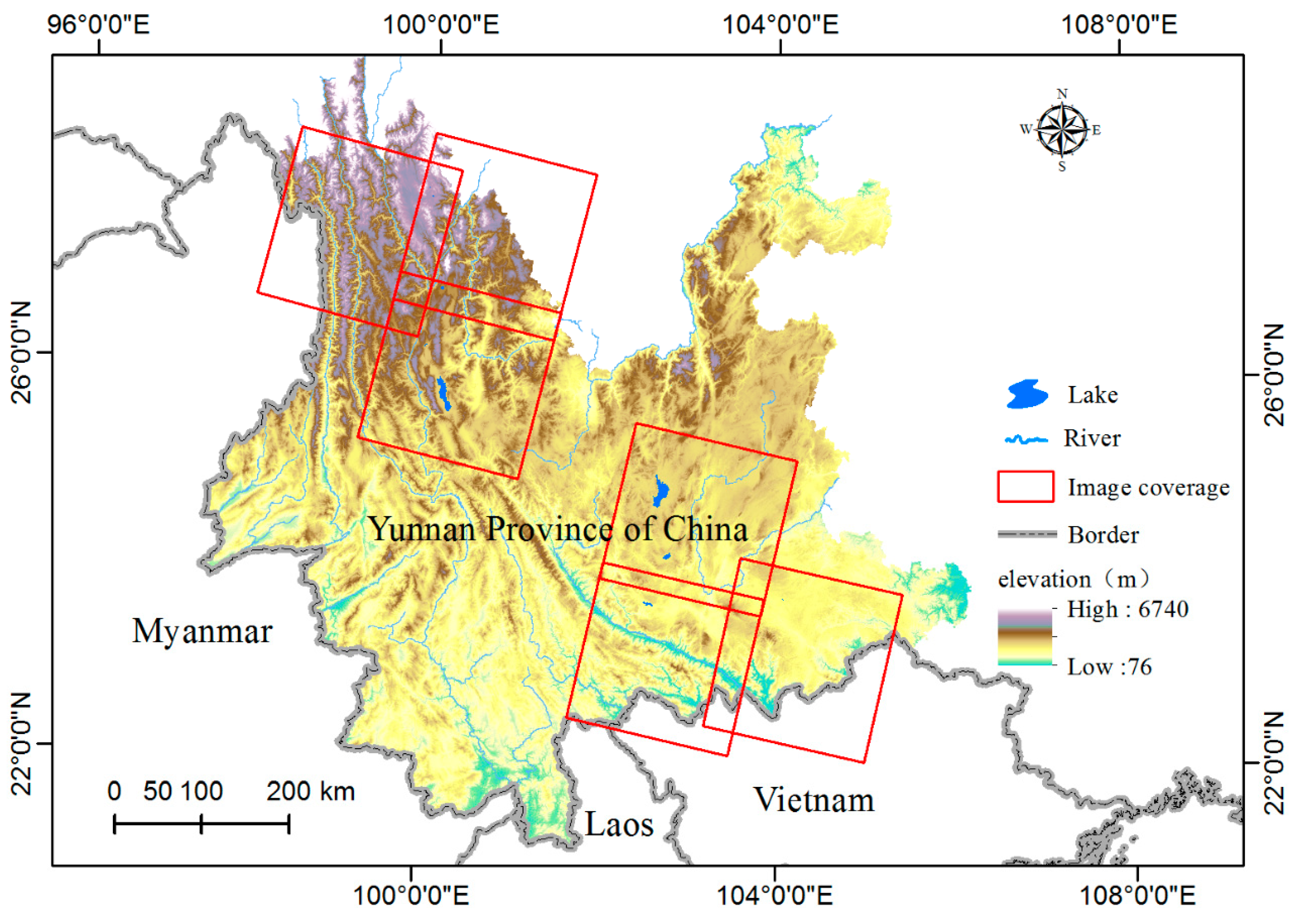
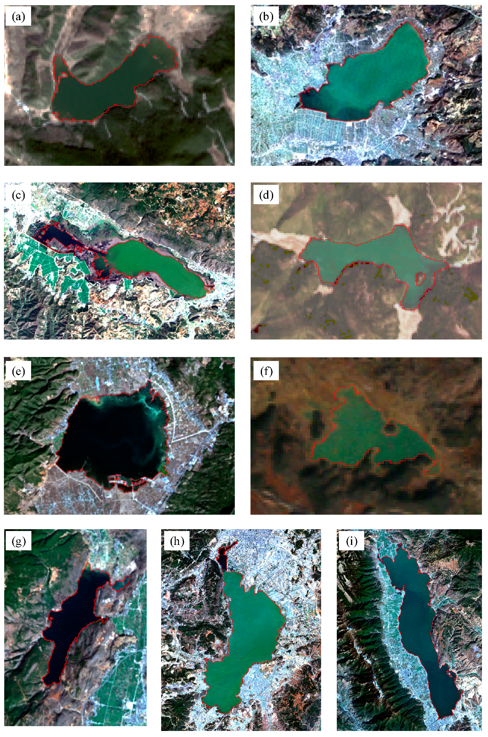
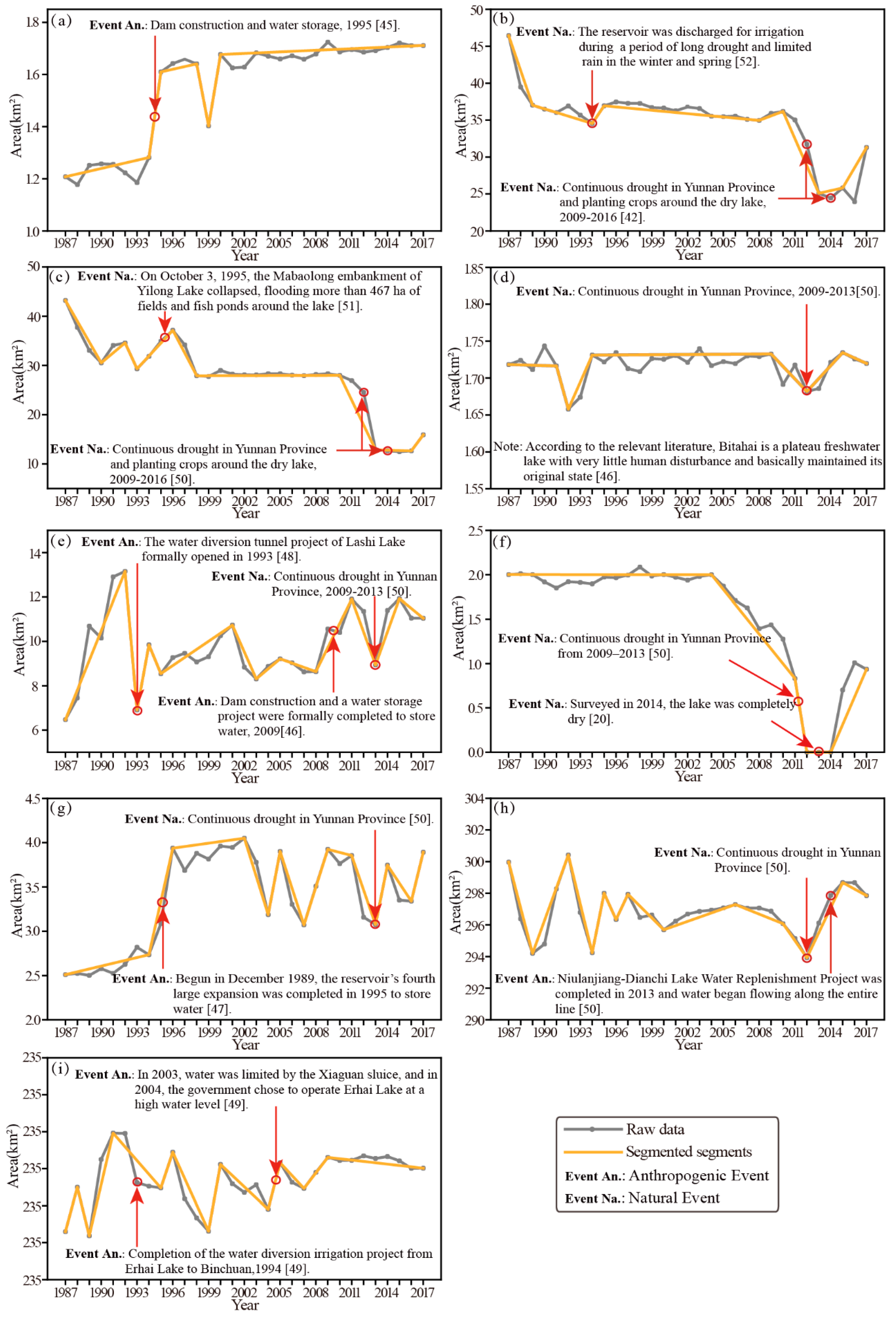
Analysis of a time series curve plotted with sufficiently continuous lake area data not only effectively reflects the lake area variation trend but also captures any major lake disturbance events. In this study, the input data used to construct the time series curve were the annual average lake area measurements extracted from the remote sensing images during each dry season (November to April of the next year) from 1987 to 2017.

3.2. Time Series Lake Surface Area Curve Segmentation and Identification of Disturbance Events

(1) Simplification of the time series curve using the Douglas-Peucker algorithm

The occurrence of large natural or human activities in (or around) a lake will cause lake area disturbances. For example, dam construction or water storage in a lake will cause a sudden increase in lake area, whereas land reclamation around a lake will cause a rapid decrease in lake area. Furthermore, strong natural events such as rainfall or drought can also cause increases or decreases in lake area. Such event-induced lake changes manifest as sudden changes in the time series lake surface area curve. However, minor events or precipitation differences will also cause variations in the time series curve. These changes are not key factors affecting the lake area but may be obstacles to the identification of key disturbances; thus, they are considered noise that should be removed for the time-series analysis.

Several methods, such as LandTrendr [35], CCDC [36] and BFAST [37], have been proposed to identify disturbances using remotely sensed time series indices (such as NDVI (Normalized Difference Vegetation Index), NBR (Normalized Burn Ratio), TCA (Tasselled Cap Angle). However, most of the lake surface area time series appear to be purely random and nonstationary time series (see

Table 2. The ADF (Augmented Dickey-Fuller) test to lake surface area time series of the nine lakes.

Lake	ADF Test (at 0.05 Level)	Stationary (yes/no)
Shudu lake	P = 0.5355 > 0.05	no
Qilu Lake	P = 0.341 > 0.05	no
Yilong Lake	P = 0.1825 > 0.05	no
Bitahai Lake	P = 0.03192 < 0.05	yes
Lashihai Lake	P = 0.04617 < 0.05	yes
Yuxian Lake	P = 0.3644 > 0.05	no
Haixihai Lake	P = 0.5563 > 0.05	no
Dianchi Lake	P = 0.01 < 0.05	yes
Erhai Lake	P = 0.1577 > 0.05	no

); unlike indices such as NDVI, NBR and TCA, lake surface areas are limitless (there is theoretically no upper boundaries for lake areas), which means existing models, such as LandTrendr, CCDC, and BFAST, are theoretically unsuitable (or could not be directly used) for the analysis of lake surface area time series. Fortunately, the Douglas-Peucker (D-P) line simplification algorithm, which is used to eliminate low-intensity noises and smooth minor changes on the curve to better capture larger changes on the curve, is an appropriate alternative.

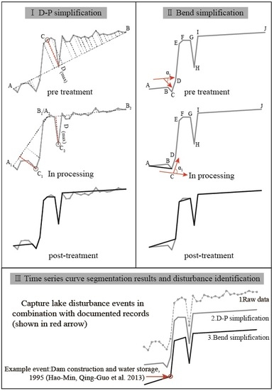
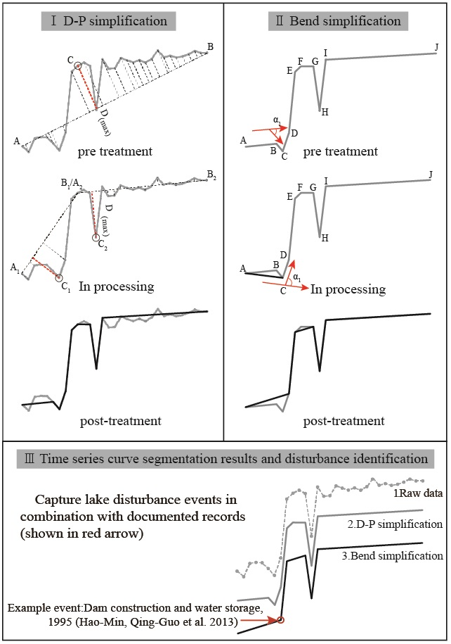
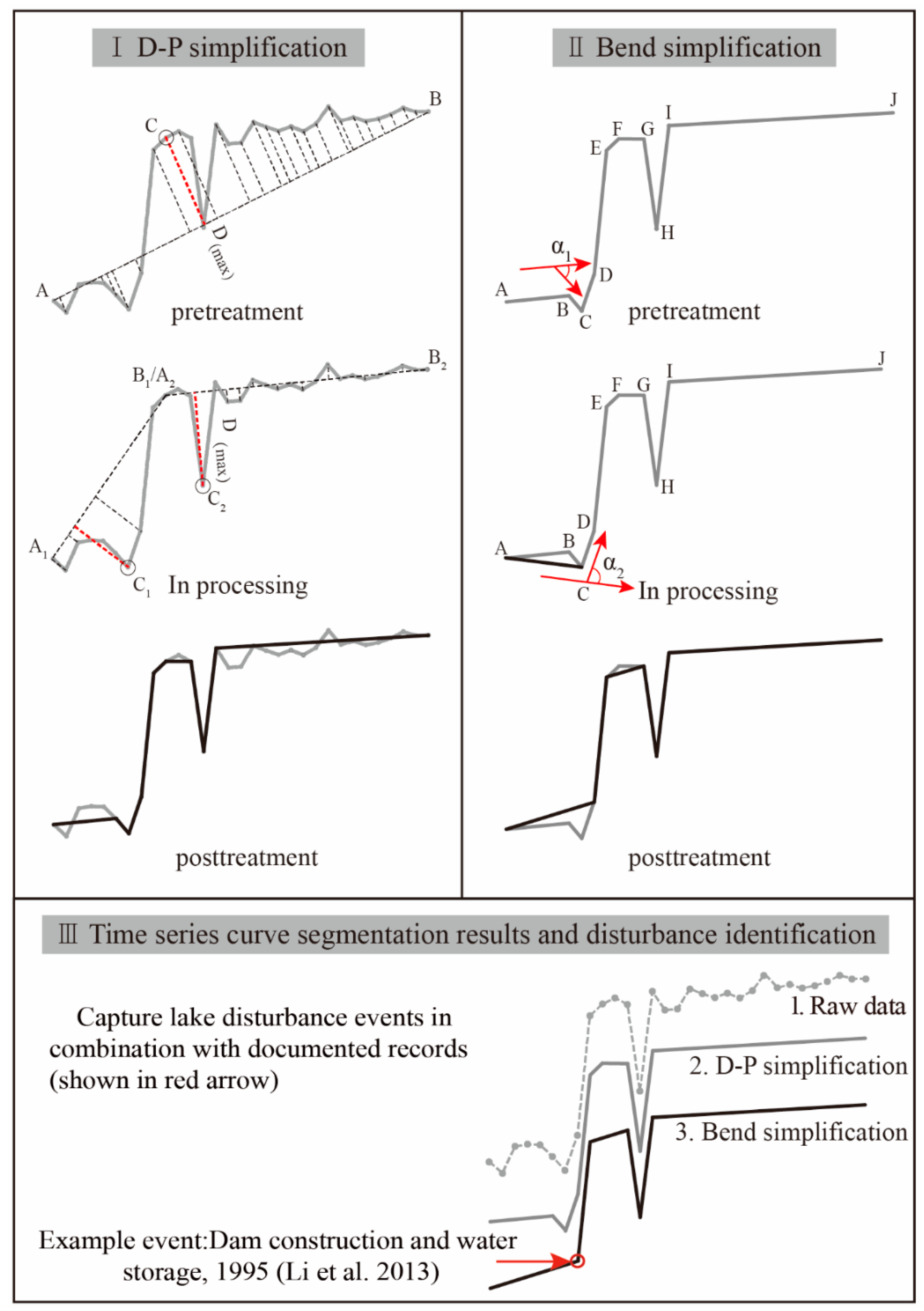
The D-P algorithm was proposed by Douglas and Peucker in 1973 [26]. Currently, this algorithm is recognized as a classical algorithm for vector line simplification in GIS (geographic informational system). The basic idea of the algorithm is as follows: (1) line AB (see Figure 2) connects the two end points A and B of a time series curve, forming the chord of the curve; (2) for each of the points (for example, point C) between A and B on the curve, there will be a distance to this chord (to line AB), forming a set of distances D, and the maximum distance of D is d(max); (3) d(max) is then compared with the given tolerance ε, and if d(max) is smaller than ε, then line AB is taken to be the approximation of the curve, and the processing of this curve section ends, but if d(max) is larger than ε, then the corresponding point (point C) is used to divide the curve into two subsegments (AC and BC), and each of the two subsegments is further processed following steps 1 through 3 until each of their d(max) values is less than the given ε; (4) after all the curves are processed, the segmentation points are connected sequentially to form a polyline that represents a simplification of the curve.

(2) Bend simplification and time series curve segmentation

After D-P simplification of the time series curve, several minor-change points may not have been removed. As these points are not indicative of major lake disturbances, they should be removed. To retain only the feature points with the main fluctuations on time series curves, we used the bend simplification algorithm, which can eliminate smaller fluctuations [38], to simplify the D-P algorithm simplified curve.

The bend simplification algorithm was used to determine whether the variation in the curvature at each point is smooth. Given a predefined threshold, if the curvature was smaller than the threshold, the point was eliminated and a new segment was created between the two points adjacent to the eliminated point. However, if the curvature exceeded the predefined threshold, the corresponding point was considered a potential feature point and was retained. After each point was processed, the retained potential points were then connected sequentially to form the finally simplified time series curve. The specific steps of the bend simplification algorithm are illustrated in Figure 2 and are explained as follows: (1) first, we calculated the curvatures on each point of the curve except for the first and last points; (2) second, for the curvature on the second point (for example point B), the two adjacent points A and C were used to construct vectors AB and BC, and the angle formed by these two vectors was calculated as α1; if α1 was larger than the preset threshold α, the curvature on point B was considered to be large and was retained as a key point; however, if the angle α1 between vector AB and BC was less than the preset threshold α, point B was removed. Following the steps above, curvatures on point C, D, etc. were judged one by one; (3) after step (2), all points, except the beginning and the end points, that meet the given curvature threshold α were retained as feature points that are representative of the main lake surface area change events.

(3) Feature extraction and disturbance identification

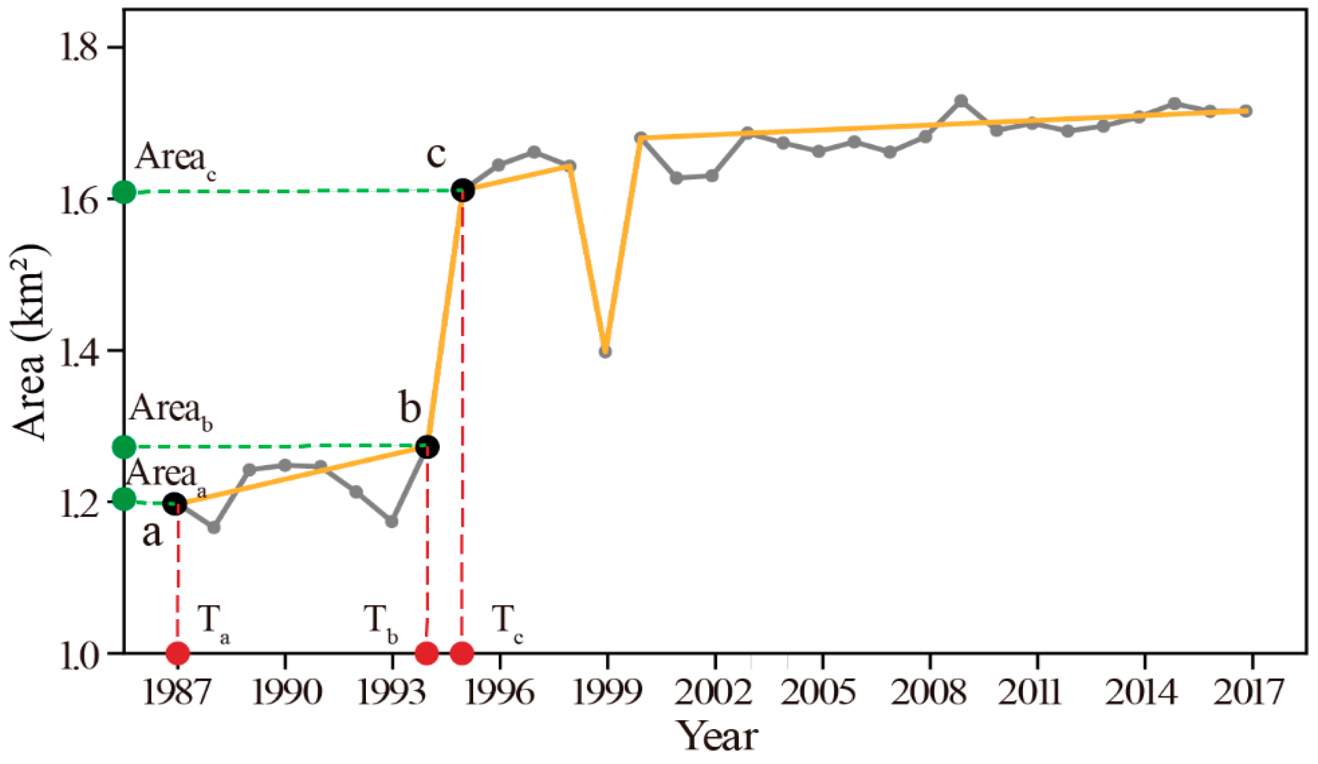
By setting appropriate segmentation parameters, disturbances that were considered “major” by users were obtained. For the segmented time series, each segment represents different lake disturbance events. When the lake was greatly disturbed by major influences, the variation in the time series curve was distinguishable. According to the segmented curves, lake surface disturbance features such as the trajectory, duration and recovery rate were extracted to classify each disturbance following an unsupervised clustering method. For these extracted features, the trajectory here was defined as the curve that formed by lake surface areas changing with time. To quantify disturbances within each trajectory, we defined two indicators: disturbance duration and disturbance recovery rate. For each disturbance, there were beginning and ending points, the time-span between these two points was defined as disturbance duration (if not, disturbance duration was defined as infinity). For each disturbance, there will be a rate; the disturbance event rate was defined as the area difference between the beginning and the end of a segment divided by the disturbance duration (see Equations (2) and (3)). For each disturbance, there were two adjacent segments. The recovery rate was the area change ratio between prior segment and the next (see Equations (4) and (5)). Features we used for disturbance classification are as follows:

Feature event rate:

$$\mathrm{Event}\mathrm{rate}1=\left|{\mathrm{Area}}_a-{\mathrm{Area}}_b\right|/\left(T_b-T_a\right)$$

(2)

$$\mathrm{Event}\mathrm{rate}2=\left|{\mathrm{Area}}_c-{\mathrm{Area}}_b\right|/\left(T_b-T_c\right)$$

(3)

Feature recovery rate:

$$\mathrm{Area}\_{\mathrm{Diff}}_{ab}=\mathrm{Max}\left({\mathrm{Area}}_a,{\mathrm{Area}}_b\right)-\mathrm{Min}\left({\mathrm{Area}}_a,{\mathrm{Area}}_b\right)$$

(4)

$${\mathrm{Re}}_{\mathrm{rate}}=\left({{\mathrm{Area}}_{\mathrm{Diff}}}_{ab}-{{\mathrm{Area}}_{\mathrm{Diff}}}_{bc}\right)/\mathrm{Max}\left({\mathrm{Area}}_{\mathrm{Diff}}{}_{ab},{\mathrm{Area}\_\mathrm{Diff}}_{bc}\right)$$

(5)

where ${\mathrm{Area}}_a$ represents the lake area at point a and $T_a$ is the time (year) of disturbance at point a; $\mathrm{Area}\_{\mathrm{Diff}}_{ab}$ denotes lake surface area difference between point a and point b; $\mathrm{Re}\_\mathrm{rate}$ is disturbance recovery rate for disturbance at point b, details are as illustrated in Figure 3.

Unlike trajectory classifications of disturbances in forests, lake disturbance classifications are small sample-based classification tasks, because major lake surface area disturbances are small probability events that cause training sample insufficiency of classifiers, such as statistical classifiers, machine learning classifiers or artificial intelligence classifiers. Therefore, we used the k-means clustering [39] method to classify disturbances into anthropogenic or natural events.

(4) Lake surface area disturbance identification accuracy assessment

Disturbance identification accuracy was determined using the confusion matrix, which uses overall accuracy (OA) to represent the percentage of correctly classified disturbances, the user’s accuracy (UA) to denote how well training-set samples are classified, and the producer’s accuracy (PA) to show the probability that a classified sample represents a given class in reality [40]. In this study, we used $U{A}_{ad}$ and $U{A}_{nd}$ to represent the user’s accuracies of anthropogenic disturbances and natural disturbances and the $P{A}_{ad}$ and $P{A}_{nd}$ to represent the producer’s accuracies of anthropogenic disturbances and natural disturbances (see

Table 3. Classification accuracy assessment indices and formulas.

Producer’s Accuracy		User’s Accuracy		Overall Accuracy	F-Score
Anthropogenic Disturbances	Natural Disturbances	Anthropogenic Disturbances	Natural Disturbances
${\mathrm{PA}}_{\mathrm{ad}}=\frac{\mathrm{TP}}{\mathrm{TP}+\mathrm{FN}}$	${\mathrm{PA}}_{\mathrm{nd}}=\frac{\mathrm{TN}}{\mathrm{TN}+\mathrm{FP}}$	${\mathrm{UA}}_{\mathrm{ad}}=\frac{\mathrm{TP}}{\mathrm{TP}+\mathrm{FP}}$	${\mathrm{UA}}_{\mathrm{nd}}=\frac{\mathrm{TN}}{\mathrm{FN}+\mathrm{TN}}$	$\mathrm{OA}=\frac{\mathrm{TP}+\mathrm{TN}}{\mathrm{TP}+\mathrm{TN}+\mathrm{FP}+\mathrm{FN}}$	$F=2\frac{{\mathrm{PA}}_{\mathrm{ad}}{\mathrm{UA}}_{\mathrm{ad}}}{{\mathrm{PA}}_{\mathrm{ad}}+{\mathrm{UA}}_{\mathrm{ad}}}$

). We employed the method given by Adeline et al. [41] to evaluate the disturbances identification accuracy levels, and validation samples were randomly selected from the documented disturbance event records. Reference data and predicted results of the confusion matrix were defined as TP (true positive), TN (true negative), FP (false positive) and FN (false negative). TP denotes the number of correctly classified as anthropogenic disturbances, TN is the number of correctly detected as natural disturbances, FP represents the number of natural disturbances misclassified as anthropogenic disturbances and FN is the number of anthropogenic disturbances misclassified as natural disturbances. As the F-score strikes a good balance between under- and over-detection accuracy levels, it was used in this study to evaluate the accuracy of the methods used (see Table 3).

4. Results and Discussion

4.1. Accuracy Evaluation of Extracted Lake Surface Area

The SAR and the MNDWI-based lake surface area extraction results of the nine chosen lakes are shown in

Table 4. Accuracies of different lake water extraction results.

Lakes	Landsat-OLI	Area (km²)	Sentinel-1A	Area (km²)	Area Differences (km²)
Shudu Lake	02/15/2017	1.69	02/10/2017	1.69	0.00
Qilu Lake	03/14/2017	32.12	03/13/2017	30.99	1.13
Yilong Lake	03/14/2017	18.21	03/13/2017	17.33	0.88
Bitahai Lake	02/15/2017	1.61	02/10/2017	1.59	0.02
Lashihai Lake	02/03/2015	12.28	01/30/2015	11.25	1.03
Yuxian Lake	03/23/2017	0.96	03/22/2017	0.91	0.04
Haixihai Lake	02/08/2017	3.77	02/10/2017	3.55	0.22
Dianchi Lake	03/14/2017	298.32	03/13/2017	295.42	2.90
Erhai Lake	02/08/2017	242.34	02/10/2017	241.35	0.98

. Compared with the Sentinel-1 data extracted lake areas, the maximum bias was 0.0918% for Lashihai Lake and the minimum bias was 0.0016% for Shudu Lake, and each of the nine lakes had a bias of less than 0.1% between the Sentinel-1 and the OLI extracted results. The extracted annual lake area data with a small bias and the Sentinel-1 extracted lake areas were used to establish a reliable time series curve. Landsat-derived lake surface areas are presented in Figure 4.

4.2. Time Series Curve Segmentation Accuracy Assessment

4.2.1. Parameter Tuning for Time Series Surface Area Curve Segmentation Method

To identify major lake surface area disturbances, the time series curve segmentation method removes small fluctuations but keeps major inflection points by setting thresholds for our curve segmentation method. There are two primary thresholding steps in our method, one for the D-P algorithm and the other for the bend simplification algorithm. Using a preset tolerance ε for D-P algorithm and the angle threshold α, the time series curve were segmented. The input data for the bend simplification algorithm were the data simplified by the D-P algorithm; therefore, it was especially important to select the threshold for the D-P algorithm. A high threshold for the D-P algorithm will result in important lake disturbance information losses, but a low threshold value will cause overfitting. Figure 5 shows the schematic diagram of the threshold selection for the time series curve segmentation, and panels 5(a), 5(b), 5(c), and 5(d) show the segmentation results from the D-P algorithm used with different thresholds. As shown in Figure 5, the threshold of 5(a) is too small and failed to reject most of the small variations that are not considered major disturbances. However, a high threshold value will result in the loss of major disturbances. Only the threshold of 0.06 set in panel 5(b) is reasonable in that it not only rejects several small variations but also maintains the major fluctuations.

As there are still several small fluctuations not removed by the D-P simplification, the bend simplification algorithm is used to further simplify the segments obtained by the D-P algorithm. As shown in Figure 5e, when the threshold α for the bend simplification algorithm was too low, several small fluctuations were not eliminated. However, a greater threshold will cause several major disturbances to be eliminated, as shown in Figure 5g,h. A threshold of 12.5 set in Figure 5f is reasonable in that it not only maintains the large fluctuations but also rejects the small fluctuations. Thresholds used in this study are as listed in

Table 5. Tuning of time series curve segmentation parameters and their accuracies.

Lake	Maximum Area (km²)	Minimum Area (km²)	Area Difference (km²)	Threshold ε for D-P	Threshold α for Bend Simplification
Shudu lake	1.72	1.19	0.54	0.06	12.50
Qilu lake	46.44	23.96	22.48	3.00	17.50
Yilong lake	43.21	12.49	30.71	3.50	19.50
Bitahai lake	1.64	1.56	0.09	0.03	23.00
Lashihai lake	13.15	6.47	6.68	1.50	25.00
Yuxian lake	2.01	0.00	2.01	0.45	11.50
Haixihai lake	4.05	2.50	1.55	0.35	18.00
Dianchi lake	300.42	293.92	6.50	1.60	28.50
Erhai lake	244.90	237.96	6.94	1.15	13.50

for the D-P and bend simplification algorithms for segmenting the curves of the nine lakes. For the D-P algorithm, the threshold was set to a value between 0.1 to 0.35 times the difference between the maximum and the minimum value on the curve. The threshold α for the bend simplification algorithm was set between 10° and 30° to obtain the optimum threshold. Tuning of segmentation parameters is critical to disturbance identification, although manual tuning is reliable in segmentation precision, its time and labor consuming remains a major obstacle.

4.2.2. Time Series Curve Segmentation Results

The time series curve segmentation algorithm is key for identifying disturbances based on time series remote sensing observations [42]. However, noise caused by the lake surface extraction method, seasonal variation in the lake areas, random precipitation, etc., in the time series curve is the main obstacle to time series curve-based analysis. Smoothing or simplification of a time series curve is needed to extract the features of disturbances from the curve [43].

After the D-P and bend simplification processing, segments that represent major lake surface disturbances are obtained; these segments indicate the duration, amplitude, beginning and ending time, etc., of each disturbance and are further used in the disturbance type classification. This is a key step for accurately identifying the disturbances. This study used the simple and easy operational threshold determination method to simplify and segment the time series curves. As shown in Figure 6, the time series of lake surface area of the nine chosen lakes were segmented into 51 segments using our curve segmentation method and 19 records are marked in the results, indicating that our method could accurately locate these disturbances, including those from anthropogenic activities, such as reservoir constructions, irrigations, dam constructions, water storage projects and natural factors, such as droughts and heavy rainfalls.

This study used yearly Landsat-extracted lake surface area data to construct the time series curve from 1987 to 2017. According to the 19 lake disturbance records, the 18 recorded disturbance dates are consistent with the segmentation results, for a total accuracy of 94.73%.

4.3. Lake Surface Area Disturbance Feature Extraction and Identification

4.3.1. Lake Surface Area Disturbance Feature Extraction

Inland lakes vary in area and morphology; this is often the result of human activities or natural factors [44]. The spatial and temporal characteristics can provide sufficient information to distinguish these two kinds of lake surface area variations. To classify these major lake surface area changes into anthropogenic or natural events, we extracted the lake surface area features based on the segmented time series and the documented lake change records. We found 19 officially documented lake change records (including three repeated records during the same disturbances) for the nine lakes (see Figure 6); according to these references, anthropogenic lake surface area disturbances included reservoir constructions [45,46,47], irrigation [48,49], transforming lakes into fields [50], etc., and natural events included droughts and heavy rainfalls [51], such as the severe drought from 2009 to 2013 in Yunnan Province [50,52].

Documented events and their characteristics of change on the time series curves are shown in Figure 6, and these distinguishable features can be summarized as follows: (1) human-induced lake surface area changes will cause an abrupt increase (or decrease) in the time series curve and the area increments are commonly larger for anthropogenic events compared to those for the natural disturbances, for example, due to anthropogenic activities, the lake surface area for Shudu Lake increased to 1.4 times that of 1993 between 1993 and 1995, the lake area of Lashihai Lake in 1993 increased to 2.03 times that of 1992, Yuxian Lake became 2.1 times larger in 2011 than it was 2006, and Haixihai Lake was in 1.4 times larger in area in 1996 than it was in 1994. In contrast, natural disturbances-induced lake area changes for Shudu Lake between 1998 and 1999, Bitahai Lake between 1990 and 1992, Lashihai Lake between 2010 and 2013 and Haixihai Lake between 2010 and 2013 were 1.2, 1.1, 1.1 and 1.2 times the areas, respectively. The increased areas rarely revert to their original level in a short period of time (years) for these anthropogenic disturbances. (2) For natural disturbances, there are abrupt increases (or decreases) on the time series curves as well, but these increments (or decreases) tend to decrease (or increase) to their original level at the end of a disturbance; therefore, these disturbances show a ‘V’ (or ‘Ʌ’) shape on the time series curves, and these natural event-caused changes typically consist of two parts, a change and a recovery, and the recovery is commonly missing from anthropogenic disturbances.

In this study, a total of 51 segments were generated for the nine lake surface area time series; there was at least one major event for each of these lakes, either anthropogenic or natural. These disturbances caused remarkable fluctuations on the time series curves, and according to the shape of each fluctuation on the time series curves, fluctuations with remarkable durations indicate that there are close correlations between the current events and their adjacent procedures. Based on this characteristic of each disturbance and using these records as references, we defined and extracted the semantic features for each disturbance. Considering the adjacent procedure deficiency for disturbances segmented at the beginning or end of the curves, disturbances on the beginning or end of the curves were ignored. As a result, 51 disturbances in total were classified.

4.3.2. Classification Results of Lake Surface Area Disturbances

For major disturbances, the documented records indicated that anthropogenic disturbances tend to not recover to their original level within a short duration of several years after a disturbance, such as the dam construction of Shudu Lake in 1995; after the water storage of the lake, water surface area never falls back to its original level again. However, natural disturbances had evident recover and mostly returned to their original levels, such as after the collapse of the Mabaolong embankment of Yilong Lake in October 1995, when the lake area soon decreased to its original level after less than 2 years. Although the defined features worked well for identifying most of the disturbances, errors remained as there were still exceptive natural (anthropogenic) disturbances had the similar trajectory as anthropogenic (natural) disturbances. As shown in

Table 6. Disturbance classification features and the classification results of the 16 records (An.: Anthropogenic event, Na.: Natural event).

Lake	Time	Event Rate 1	Event Rate 2	Area_Diff	Re_Rate	Documented Disturbance	Classified Disturbance
Shudu Lake	1994–1998	0.6002	0.0188	0.0314	0.9059	An.	An.
Qilu Lake	1989–1995	0.0221	0.1066	0.2072	0.0346	Na.	Na.
Qilu Lake	2010–2017	0.1304	0.1017	0.7792	0.4156	Na.	Na.
Yilong Lake	2010–2017	0.1640	0.0332	0.2022	0.7978	An.	An.
Yilong Lake	1993–1996	0.0849	0.1502	0.5653	−0.1521	Na.	Na.
Bitahai Lake	2009–2015	0.1982	0.2053	0.9658	−0.0342	Na.	Na.
Lashihai Lake	1992–1994	0.3116	0.1467	0.4707	0.5293	An.	An.
Lashihai Lake	2008–2011	0.1629	0.2216	0.7351	0.0931	An.	Na.
Lashihai Lake	1994–2001	0.2216	0.2235	0.9917	0.0083	Na.	Na.
Yuxian Lake	2011–2012	0.3986	0.2243	0.5628	−0.1255	Na.	Na.
Haixihai Lake	1994–1996	0.3882	0.0121	0.0313	0.9062	An.	An.
Haixihai Lake	2011–2014	0.2516	0.4329	0.5812	0.1398	Na.	Na.
Dianchi Lake	2012–2015	0.2439	0.0636	0.2607	0.8262	An.	An.
Dianchi Lake	2012–2017	0.1658	0.2439	0.6797	−0.5469	Na.	Na.
Erhai Lake	1991–1995	0.1336	0.3483	0.3835	0.3482	An.	Na.
Erhai Lake	2004–2005	0.4536	0.1254	0.2764	0.4472	An.	An.

, disturbance of Erhai Lake in 2003 was caused by governmental water storage charge with both quick water storage and release process. Another limitation for the current method is to classify disturbances that were caused by both natural and anthropogenic events, such as the drought in 2009–2013 in Yunnan Province, where water shortage compel irrigation by the locals from lakes, It is challenging to figure out which is the dominant factor the lake surface area shrinkage: natural or anthropogenic?

The classified disturbance types agreed well with the records according to the accuracy assessment results in

Table 7. Anthropogenic (An.) and Natural (Na.) disturbance identification accuracy assessment.

Producer’s Accuracy (%)		User’s Accuracy (%)		Overall Accuracy (%)	F(ad)-Score	F(nd)-Score
An.	Na.	An.	Na.
100	80	75	100	87.5	85.71	88.89

; among the 16 recorded disturbances, two anthropogenic disturbances were misclassified as natural disturbances, and the overall identification accuracy was 87.75%, with an F-score of 85.71 for anthropogenic disturbances and 88.89 for natural disturbances. This result suggests the reliability of our proposed method.

During the past 31 years, there were 51 major disturbances for the nine lakes in Yunnan Plateau, and only nine segments were with no major disturbances (see Figure 6 and

Table 8. Statistics on the number of disturbances caused by different factors.

Lake Name	Anthropogenic Disturbances (times)	Natural Disturbances (times)	No Disturbances	Total
Shudu lake	1	1	1	3
Qilu lake	4	0	2	6
Yilong lake	1	2	1	4
Bitahai lake	1	1	1	3
Lashihai lake	7	1	1	9
Yuxian lake	1	1	1	3
Haixihai lake	2	4	1	7
Dianchi lake	4	2	1	7
Erhai lake	4	5	0	9
Total	25	17	9	51

). Among these disturbances, up to 25 were human-induced, and these disturbances had a major impact on lake surface area change. Human-induced disturbances are commonly ‘irreversible’, because lake surface area will not revert to its original levels within a short period of time; for example, lake surfaces for Shudu Lake between 1993 and 1995, Qilu Lake between 2010 and 2015, Yilong Lake between 2010 and 2016, Lashihai Lake between 1992 and 1993, Yuxian Lake between 2006 and 2011 and Haixihai Lake between 1994 and 1996 increased (or decreased) to 1.4, 1.5, 2.2, 2.03, 2.1 and 1.4 times their original areas, respectively. Yuxian Lake completely dried between 2011 and 2014 because of human activities, including reclaiming land from this lake and irrigation [20,50]. These results indicated that the human-induced disturbances tend to be durable.

In our study period, natural event-induced major lake surface area disturbances occurred 17 times, almost half of the human induced disturbances. These disturbances were less impactful, because lake surface areas reverted to their original levels after these disturbances and, therefore, these disturbances were not long lasting. For example, natural disturbances for Shudu Lake between 1998 and 1999, Bitahai Lake between 1990 and 1992, Lashihai Lake between 2010 and 2013 and Haixihai Lake between 2010 and 2013, caused lake surface area increases (or decreases) to 1.2, 1.1, 1.1 and 1.2 times their original levels, respectively. The lakes with natural disturbances had less of an increment (or decrement) compared to those with the human activity-induced disturbances, and they reverted to their original levels after a short period of time (within 2 years in this study). In our study area, each of the lakes, except Bitahai Lake, had large human activity-induced disturbances, and there were much more anthropogenic disturbances for Lashihai Lake, Erhai Lake, Dianchi Lake and Qilu Lake. According to the documented records, most of these human activities were dam construction, irrigation and land reclamation.

5. Conclusions

In this study, annual Landsat remote sensing images taken during the dry seasons from 1986 to 2017 were used to extract lake surface area information for nine typical lakes in Yunnan Province, China. To identify whether human activity or natural events dominate inland lake surface change, we proposed a method based on the D-P simplification algorithm combined with the bend simplification method to locate large lake change events and then characterize the features of change for each event to classify them into anthropogenic or natural lake surface area disturbances. Based on validation data from a documented governmental report and year book, we assessed the accuracy of our method for both the disturbance location and the disturbance identification, and the results are as follows:

(1)

The method can accurately locate the main lake changing events based on the time series lake surface area curve. When a large disturbance event occurs for a lake, its area will also increase (or decrease). The method proposed in this paper effectively eliminates noise in the time series of lake surface area using the combined D-P simplification algorithm and bend simplification algorithm. This method retains the large mutation points in the time series lake surface area curve and accurately locates the lake changing events within the time series lake surface curve; the temporal accuracy of this model for segmenting the lake area time series curves was 94.73% in our study.

(2)

To characterize the disturbances on each time series curve, we extracted the disturbance classification features, including the amplitude (event rate), duration and trajectory (recovery rate). Using the k-means clustering method, we achieved an overall accuracy of disturbance identification of 87.75%, with an F-score of 85.71 for anthropogenic disturbances and 88.89 for natural disturbances.

(3)

According to our results, lakes in Yunnan Province, China, have undergone extensive disturbances, and the human-induced disturbances occurred almost twice as often as natural disturbances, indicating intensified disturbances caused by human activities, such as reservoir constructions, irrigation, turning lakes into fields, etc. Worse still, the anthropogenic disturbances appear to be lasting compared with the natural disturbances. Lakes subjected to natural disturbances tend to recover within a short period of time, while lakes subjected to anthropogenic disturbances had longer recovery times or never recovered.

Because the available remote sensing image data of satisfactory cloud-free quality from the study period are predominantly concentrated during Yunnan’s dry season, the data selected were all from November to April. In future studies, multisensor spatial-temporal fusion techniques and radar remote sensing image data should be combined to obtain year-round lake water areas to comprehensively analyze the annual variation characteristics to more accurately capture lake disturbance events.

References

1. Ding, Y.; Liu, S.; Ma, Y.; Ye, B.; Zhao, L. Climatic implications on variations of lakes in the cold and arid regions of china during the recent 50 Years. J. Glaciol. Geocryol. 2006, 28, 623–632. [Google Scholar] [CrossRef]
2. Pekel, J.F.; Cottam, A.; Gorelick, N.; Belward, A.S. High-resolution mapping of global surface water and its long-term changes. Nature 2016, 540, 418–422. [Google Scholar] [CrossRef]
3. Yamazaki, D.; Trigg, M.A.; Ikeshima, D. Development of a global ~90m water body map using multi-temporal Landsat images. Remote Sens. Environ. 2015, 171, 337–351. [Google Scholar] [CrossRef]
4. Moser, K.A.; Baron, J.S.; Brahney, J.; Oleksy, I.A.; Saros, J.E.; Hundey, E.J.; Sadro, S.A.; Kopáček, J.; Sommaruga, R.; Kainz, M.J.; et al. Mountain lakes: Eyes on global environmental change. Glob. Planet. Chang. 2019, 178, 77–95. [Google Scholar] [CrossRef] [Green Version]
5. Vorosmarty, C.J.; Green, P.; Salisbury, J.; Lammers, R.B. Global water resources: Vulnerability from climate change and population growth. Science 2000, 289, 284–288. [Google Scholar] [CrossRef] [Green Version]
6. Huang, C.; Chen, Y.; Zhang, S.; Wu, J. Detecting, extracting and monitoring surface water from space using optical sensors: A review. Rev. Geophys. 2018, 56, 333–360. [Google Scholar] [CrossRef]
7. Luo, K.; Tao, F. Monitoring of forest virtual water in Hunan Province, China, based on HJ-CCD remote-sensing images and pattern analysis. Int. J. Remote Sens. 2016, 37, 2376–2393. [Google Scholar] [CrossRef]
8. Tulbure, M.G.; Broich, M.; Stehman, S.V.; Kommareddy, A. Surface water extent dynamics from three decades of seasonally continuous Landsat time series at subcontinental scale in a semi-arid region. Remote Sens. Environ. 2016, 178, 142–157. [Google Scholar] [CrossRef]
9. Colgan, M.; Baldeck, C.; Féret, J.-B.; Asner, G. Mapping Savanna Tree Species at Ecosystem Scales Using Support Vector Machine Classification and BRDF Correction on Airborne Hyperspectral and LiDAR Data. Remote Sens. 2012, 4, 3462–3480. [Google Scholar] [CrossRef] [Green Version]
10. Peng, J.; Jia, J.; Liu, Y.; Li, H.; Wu, J. Seasonal contrast of the dominant factors for spatial distribution of land surface temperature in urban areas. Remote Sens. Environ. 2018, 215, 255–267. [Google Scholar] [CrossRef]
11. Feng, L.; Hou, X.; Zheng, Y. Monitoring and understanding the water transparency changes of fifty large lakes on the Yangtze Plain based on long-term MODIS observations. Remote Sens. Environ. 2019, 221, 675–686. [Google Scholar] [CrossRef]
12. Che, X.; Feng, M.; Jiang, H.; Xiao, T.; Wang, C.; Jia, B.; Bai, Y. Detection and analysis of Qinghai-Tibet Plateau lake area from 2000 to 2013. Geo Inf. Sci. 2015, 17, 97–107. [Google Scholar] [CrossRef]
13. Mcfeeters, S.K. The use of the Normalized Difference Water Index (NDWI) in the delineation of open water features. Int. J. Remote Sens. 1996, 17, 1425–1432. [Google Scholar] [CrossRef]
14. Feng, L.; Hu, C.; Chen, X.; Cai, X.; Tian, L.; Gan, W. Assessment of inundation changes of Poyang Lake using MODIS observations between 2000 and 2010. Remote Sens. Environ. 2012, 121, 80–92. [Google Scholar] [CrossRef]
15. Li, H.; Mao, D.; Li, X.; Wang, Z.; Wang, Z.; Wang, C. Monitoring 40-year lake area changes of the Qaidam Basin; Tibetan Plateau; using Landsat time series. Remote Sens. 2019, 11, 343. [Google Scholar] [CrossRef] [Green Version]
16. Maeda, E.; Lisboa, F.; Kaikkonen, L.; Kallio, K.; Koponen, S.; Brotas, V.; Kuikka, S. Temporal patterns of phytoplankton phenology across high latitude lakes unveiled by long-term time series of satellite data. Remote Sens. Environ. 2019, 221, 609–620. [Google Scholar] [CrossRef]
17. Wulder, M.A.; Loveland, T.R.; Roy, D.P.; Crawford, C.J.; Masek, J.G.; Woodcock, C.E.; Zhu, Z. Current status of Landsat program, science, and applications. Remote Sens. Environ. 2019, 225, 127–147. [Google Scholar] [CrossRef]
18. Xiao, Q.; Yang, K.; Hong, L. Remote sensing monitoring and temporal-spatial analysis of surface water body area changes of lakes on the Yunnan-Guizhou Plateau over the past 30 years. J. Lake Sci. 2018, 30, 1083–1096. [Google Scholar] [CrossRef]
19. Arvor, D.; Daher, F.R.G.; Briand, D.; Dufour, S.; Rollet, A.J.; Simoes, M.; Ferraz, R.P.D. Monitoring thirty years of small water reservoirs proliferation in the southern Brazilian Amazon with Landsat time series. ISPRS J. Photogramm. Remote Sens. 2018, 145, 225–237. [Google Scholar] [CrossRef]
20. Li, H.; Zang, H.; Chen, G.; Chang, F.; Duan, L.; Wang, J.; Lu, H.; Wu, H.; Hu, K. The Grain Size Distribution Characteristics of Surface Sediments from Plateau Lakes in Yunnan Province and Their Environmental Significances. Acta Sedimentol. Sin. 2017, 35, 499–507. [Google Scholar]
21. Qin, J.; Ju, J.; Xie, M. Low Latitude Plateau Weather Climate; China Meteorological Press: Beijing, China, 1997; pp. 18–19. [Google Scholar]
22. Cooley, T.; Anderson, G.P.; Felde, G.W.; Hoke, M.L.; Ratkowski, A.J.; Chetwynd, J.H.; Gardner, J.A.; Adler-Golden, S.M.; Matthew, M.W.; Berk, A.; et al. FLAASH, a MODTRAN4-based atmospheric correction algorithm, its application and validation. In Proceedings of the 2002 IEEE International Geoscience and Remote Sensing Symposium (IGARSS), Toronto, ON, Canada, 24–28 June 2002; pp. 1414–1418. [Google Scholar] [CrossRef]
23. Zhu, Z.; Woodcock, C.E. Object-based cloud and cloud shadow detection in Landsat imagery. Remote Sens. Environ. 2012, 118, 83–94. [Google Scholar] [CrossRef]
24. Zeng, L.; Schmitt, M.; Li, L.; Zhu, X. Analysing changes of the Poyang Lake water area using Sentinel-1 synthetic aperture radar imagery. Int. J. Remote Sens. 2017, 38, 7041–7069. [Google Scholar] [CrossRef] [Green Version]
25. Wang, M.; Du, L.; Ke, Y.; Huang, M.; Zhang, J.; Zhao, Y.; Li, X.; Gong, H. Impact of Climate Variabilities and Human Activities on Surface Water Extents in Reservoirs of Yongding River Basin, China, from 1985 to 2016 Based on Landsat Observations and Time Series Analysis. Remote Sens. 2019, 11, 560. [Google Scholar] [CrossRef] [Green Version]
26. Douglas, D.H.; Peucker, T.K. Algorithms for the Reduction of the Number of Points Required to Represent a Digitized Line or its Caricature. Cartogr. Int. J. Geogr. Inf. Geovis. 1973, 10, 112–122. [Google Scholar] [CrossRef] [Green Version]
27. Wang, Z.; Müller, J.C. Line generalization based on analysis of shape characteristics. Cartogr. Geogr. Inf. Syst. 1998, 25, 3–15. [Google Scholar] [CrossRef]
28. Fisher, A.; Flood, N.; Danaher, T. Comparing Landsat water index methods for automated water classification in eastern Australia. Remote Sens. Environ. 2016, 175, 167–182. [Google Scholar] [CrossRef]
29. Frazier, P.S. Water body detection and delineation with Landsat TM data. Photogramm. Eng. Remote Sens. 2000, 66, 1461–1467. [Google Scholar] [CrossRef]
30. Feyisa, G.L.; Meilby, H.; Fensholt, R.; Proud, S.R. Automated water extraction index: A new technique for surface water mapping using Landsat imagery. Remote Sens. Environ. 2014, 140, 23–35. [Google Scholar] [CrossRef]
31. Huang, X.; Hu, T.; Li, J.; Wang, Q.; Benediktsson, J.A. Mapping urban areas in China using multisource data with a novel ensemble SVM method. IEEE Trans. Geosci. Remote Sens. 2018, 56, 4258–4273. [Google Scholar] [CrossRef]
32. Otsu, N. A Threshold Selection Method from Gray-Level Histograms. IEEE Trans. Syst. Man Cybern. 1979, 9, 62–66. [Google Scholar] [CrossRef] [Green Version]
33. Xu, H. Modification of normalised difference water index (NDWI) to enhance open water features in remotely sensed imagery. Int. J. Remote Sens. 2006, 27, 3025–3033. [Google Scholar] [CrossRef]
34. Sun, G.; Chen, X.; Jia, C.; Yao, Y.; Wang, Z. Combinational Build-Up Index (CBI) for effective impervious surface mapping in urban areas. IEEE J. Sel. Top. Appl. Earth Obs. Remote Sens. 2016, 9, 2081–2092. [Google Scholar] [CrossRef]
35. Kennedy, R.E.; Yang, Z.; Cohen, W.B. Detecting trends in forest disturbance and recovery using yearly Landsat time series: 1. LandTrendr—Temporal segmentation algorithms. Remote Sens. Environ. 2010, 114, 2897–2910. [Google Scholar] [CrossRef]
36. Zhu, Z.; Woodcock, C.E. Continuous change detection and classification of land cover using all available Landsat data. Remote Sens. Environ. 2014, 144, 152–171. [Google Scholar] [CrossRef] [Green Version]
37. Verbesselt, J.; Hyndman, R.; Newnham, G.; Culvenor, D. Detecting trend and seasonal changes in satellite image time series. Remote Sens. Environ. 2010, 114, 106–115. [Google Scholar] [CrossRef]
38. Chuon, C.; Guha, S.; Janecek, P.; Nguyen, D.C.S. Simplipoly: Curvature-based polygonal curve simplification. Int. J. Comput. Geom. Appl. 2011, 21, 417–429. [Google Scholar] [CrossRef] [Green Version]
39. Hartigan, J.A.; Wong, M.A. Algorithm AS 136: A k-means clustering algorithm. J. R. Stat. Soc. Ser. C Appl. Stat. 1979, 28, 100–108. [Google Scholar] [CrossRef]
40. Congalton, R.G. A review of assessing the accuracy of classifications of remotely sensed data. Remote Sens. Environ. 1991, 37, 35–46. [Google Scholar] [CrossRef]
41. Adeline, K.R.M.; Chen, M.; Briottet, X.; Pang, S.K.; Paparoditis, N. Shadow detection in very high spatial resolution aerial images: A comparative study. ISPRS J. Photogramm. Remote Sens. 2013, 80, 21–38. [Google Scholar] [CrossRef]
42. Sulla-Menashe, D.; Kennedy, R.E.; Yang, Z.; Braaten, J.; Krankina, O.N.; Friedl, M.A. Detecting forest disturbance in the Pacific Northwest from MODIS time series using temporal segmentation. Remote Sens. Environ. 2014, 151, 114–123. [Google Scholar] [CrossRef]
43. Liu, X.; Bo, Y.; Zhang, J.; He, Y. Classification of C3 and C4 Vegetation Types Using MODIS and ETM+ Blended High Spatio-Temporal Resolution Data. Remote Sens. 2015, 7, 15244–15268. [Google Scholar] [CrossRef] [Green Version]
44. Goudie, A.S. Human Impact on the Natural Environment; Wiley: Chennai, India, 2018. [Google Scholar]
45. Li, H.; Yu, Q.; Li, N.; Wang, J.; Yang, Y. Study on Landscape Dynamics and Driving Mechanisms of the Shudu Lake Catchment Wetlands in Northwest Yunnan. J. West China For. Sci. 2013, 42. [Google Scholar] [CrossRef]
46. Yang, L.; Li, H. Yunnan Wetland; China Forestry Publishing House: Beijing, China, 2010. [Google Scholar]
47. Compilation of Eryuan County Local Chronicles Compilation Committee. Eryuan County Records: 1978–2005; Yunnan People’s Publishing House: Kunming, China, 2018. [Google Scholar]
48. Li, R. Annals of Naxi Autonomous County of Lijiang; Yunnan People’s Publishing House: Kunming, China, 2001. [Google Scholar]
49. Yan, S. Discussion on the Environmental Impact of Erhai Sea Engineering Construction. Technol. Dev. Enterp. 2014, 33. [Google Scholar] [CrossRef]
50. He, J. Yunnan Water Conservancy Yearbook; Yunnan Water Resources Department: Kunming, China, 2014. [Google Scholar]
51. Compilation of Shiping County annals Compilation Committee. Shiping County Annals: 1985–2000; Yunnan People’s Publishing House: Kunming, China, 2005. [Google Scholar]
52. Gong, P. Huaning Water Conservancy; Dehong National Publishing House: Mangshi, China, 2014. [Google Scholar]
Figure 1. Overview of the study area.
Remotesensing 12 00612 g001
Figure 2. Segmentation method for time series curves.
Remotesensing 12 00612 g002
Figure 3. Curve points used in feature extraction of times series of lake surface area.
Remotesensing 12 00612 g003
Figure 4. The extracted lake boundaries (polygon in red line) for: (a) Shudu Lake; (b) Qilu Lake; (c) Yilong Lake; (d) Bitahai Lake; (e) Lashihai Lake; (f) Yuxian Lake; (g) Haixihai Lake; (h) Dianchi Lake; (i) Erhai Lake.
Remotesensing 12 00612 g004
Figure 5. Thresholding results for: (a) to (d): Douglas-Peucker simplification algorithm; (e) to (h): bend simplification algorithm.
Remotesensing 12 00612 g005
Figure 6. Time series curve segmentation and event identification results for lake areas in the study region during the period 1987–2017. (a) Shudu Lake; (b) Qilu Lake; (c) Yilong Lake; (d) Bitahai Lake; (e) Lashihai Lake; (f) Yuxian Lake; (g) Haixihai Lake; (h) Dianchi Lake; (i) Erhai Lake.
Remotesensing 12 00612 g006