Sentinel-2 Leaf Area Index Estimation for Pine Plantations in the Southeastern United States


1
Department of Forestry and Environmental Resources, College of Natural Resources, North Carolina State University, Raleigh, NC 27607, USA
2
Center for Geospatial Analytics, North Carolina State University, Raleigh, NC 27607, USA
3
Department of Forest Resources and Environmental Conservation, Virginia Tech, Blacksburg, VA 24061, USA
*
Author to whom correspondence should be addressed.
Remote Sens. 2020, 12(9), 1406; https://doi.org/10.3390/rs12091406
Submission received: 18 March 2020
/
Revised: 18 April 2020
/
Accepted: 27 April 2020
/
Published: 29 April 2020
(This article belongs to the Section Forest Remote Sensing)
Abstract
:Leaf area index (LAI) is an important biophysical indicator of forest health that is linearly related to productivity, serving as a key criterion for potential nutrient management. A single equation was produced to model surface reflectance values captured from the Sentinel-2 Multispectral Instrument (MSI) with a robust dataset of field observations of loblolly pine (Pinus taeda L.) LAI collected with a LAI-2200C plant canopy analyzer. Support vector machine (SVM)-supervised classification was used to improve the model fit by removing plots saturated with aberrant radiometric signatures that would not be captured in the association between Sentinel-2 and LAI-2200C. The resulting equation, LAI = 0.310SR − 0.098 (where SR = the simple ratio between near-infrared (NIR) and red bands), displayed good performance ( = 0.81, RMSE = 0.36) at estimating the LAI for loblolly pine within the analyzed region at a 10 m spatial resolution. Our model incorporated a high number of validation plots (n = 292) spanning from southern Virginia to northern Florida across a range of soil textures (sandy to clayey), drainage classes (well drained to very poorly drained), and site characteristics common to pine forest plantations in the southeastern United States. The training dataset included plot-level treatment metrics—silviculture intensity, genetics, and density—on which sensitivity analysis was performed to inform model fit behavior. Plot density, particularly when there were ≤618 trees per hectare, was shown to impact model performance, causing LAI estimates to be overpredicted (to a maximum of + 0.16). Silviculture intensity (competition control and fertilization rates) and genetics did not markedly impact the relationship between SR and LAI. Results indicate that Sentinel-2’s improved spatial resolution and temporal revisit interval provide new opportunities for managers to detect within-stand variance and improve accuracy for LAI estimation over current industry standard models.

1. Introduction
Loblolly pine is the most commercially important tree species in the southeastern United States [1]. Within this region, inherent soil nutrient deficiencies of nitrogen (N) and phosphorous (P) are very common [2]. As a result, the addition of fertilizer is often a necessary silvicultural practice both at the time of planting and also at mid-rotation. Fertilization—particularly with N—has a positive correlation with leaf area index (LAI), a dimensionless ratio quantifying projected leaf surface area per unit ground area. For intensively managed loblolly pine, LAI serves as an indicator of nutrient status and potential future volume growth [3]. Higher LAIs correspond with a greater capacity to intercept light, photosynthesize and fix carbon [4].
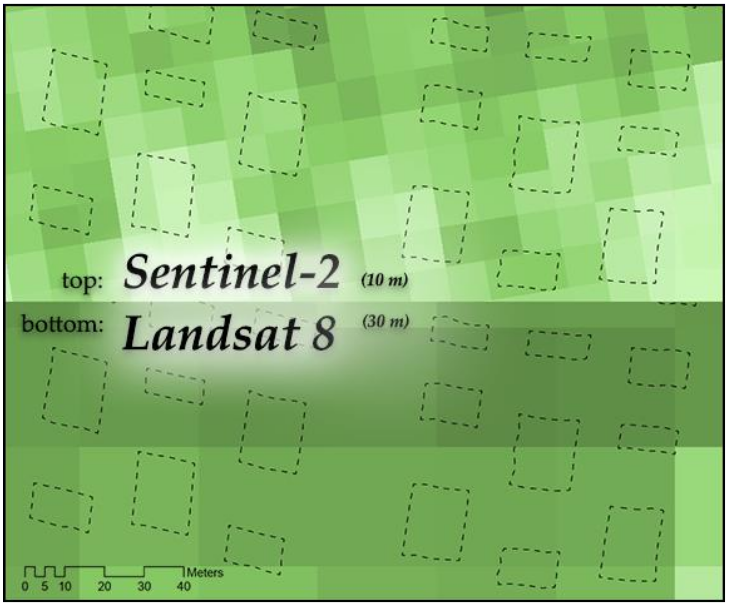
Because LAI is laborious to directly measure in the field, many forest management companies utilize satellite-derived image products to assess the LAI of their stands throughout a rotation. Commonly sourced satellites today are Landsat 7 or Landsat 8, which are operated by NASA and launched in 1999 and 2013, respectively [5]. With reliable imagery produced at a spatial resolution of 30 m with the Landsat 4 satellite since the early 1980s, the Landsat program continues to provide valuable observations of forest vegetation across the globe [6]. However, experimental forest management plots, the source of critical ground observations of quantities like LAI, are often smaller than the 30 m spatial resolution of Landsat image products (Figure A1). Forest inventory plot size widths used in this study ranged from 15 to 35 m, for instance. This discrepancy causes overlap between plot-level measurements and can lead to inaccurate and imprecise predictions [7]. Technological advances in geospatial analytics and the launch of satellites capable of retrieving data at finer resolutions with better targeted wavelength spectrums and shorter return intervals have provided the opportunity for improved LAI mapping and monitoring in forested sites.
Operated by the European Space Agency (ESA), Sentinel-2 refers specifically to two satellites—Sentinel-2A and Sentinel-2B—which have both been operationally in-orbit since the launch of Sentinel-2B in early 2017. In satellite remote sensing, leaf area index is most commonly calculated as a function of a spectral vegetation index (SVI), which is a combination of multiple spectral bands to calculate a single value [8]. Specifically, bottom-of-atmosphere reflectance values—sensor data processed to account for atmospheric distortion between the satellite sensor and at the ground—are used to analyze vegetation data such as forest canopy characteristics. Most recently, the LAI of loblolly pine was calculated via Landsat 8 satellites using the simple ratio (SR) index [9]. Compared to Landsat 8, an advantage Sentinel-2 provides for forest management is its four 10 m spatial resolution bands, which are sensitive to near-infrared (NIR), red, green, and blue electromagnetic radiation [10]. Furthermore, the five-day revisit time of Sentinel-2 creates a higher probability of producing cloudless imagery in the winter compared to the 16-day return rate for Landsat 8. This comparison between Landsat 8 and Sentinel-2 for estimating LAI has been directly explored in temperate, natural, deciduous broadleaf forests [11]. However, 20 m spatial resolution bands and many fewer field plots were used.
The LAI-2200C is a plant canopy analyzer that works by measuring diffuse radiation transmissions that reach the instrument’s sensory eye, collected within five concentric rings at a scanning angle set by the operator. The LAI-2200C is known to reliably measure the LAI when leaf angle and leaf spatial distributions are unknown or random [12]. However, it will underestimate the LAI when foliage is clumped [13,14], as is the case in loblolly pine. These shortcomings can be corrected for post-acquisition via digital transformation and implementation of clumping index and scattering correction algorithms. Still, the LAI-2200C and other canopy gap fraction based approaches do not distinguish between photosynthetically active leaf tissue and other plant materials such as branches and stems [15].
Empirical relationships modeled between remotely sensed LAI and spectral vegetation indices (LAI-SVI) do not typically generalize well across varying geography [13]. One reason for this geographic variation is variations in chlorophyll content in foliage, which could be a result of improved nutrient content from the soil, leading to less stress-related foliar variation as N becomes more readily available [13,16]. Background changes, such as moss in the summer or snow in the winter, also create spatial and temporal variations in LAI-SVI relationships [17,18,19]. Because visible background is a known issue for the retrieval of LAI and similar biophysical variables, classification may allow for the discrimination of sites saturated by undesired background content.
Support vector machine (SVM)-supervised classification works by designating a linear binary separation between designated distributions of feature inputs. Multidimensional hyperplanes are constructed as decision boundaries that minimize classification error [20]. In the case of this analysis, the feature inputs are represented as a set of radiometric signatures corresponding with each of the four bands in the composite raster image formed from the Sentinel-2 Level-2A product. The use of machine learning (ML) techniques such as SVM are becoming increasingly utilized in forested contexts to improve image classification in remote sensing [21,22]. Use-cases range from more broad remote sensing tasks of land use and land cover classification, object detection, and scene recognition, to very specific implementations such as detecting and classifying bark beetle-induced tree mortality [23,24]. The use of SVM classification has also been used extensively in the agriculture domain [25] (e.g., for identifying and separating soil pixels in the context of corn fields [26]).
No published equation currently exists that correlates in situ LAI values of loblolly pine with reflectance values produced by the various sensor bands of Sentinel-2. Further, most prior work has focused on natural forests rather than those managed. As a result, no publication has quantified plot-level treatment effects commonly used in forest management research, such as density management and genetic selection, with the resulting influence on a LAI-SVI model. Therefore, the objectives of this study were to:
- identify and model surface reflectance values captured from Sentinel-2 with field observations of loblolly pine LAI collected with a LAI-2200C;
- conduct sensitivity analysis to quantify model variance incurred from silviculture intensity, density, and genetics.
2. Materials and Methods
2.1. Research Sites and Field Data
2.1.1. Research Sites
Three research sites were included in this analysis (Figure 1).
Two of the sites—Regionwide 20 in Bladen Lakes, North Carolina (RW20-NC), and Reynold’s Homestead, Virginia (RW20-VA)—were part of an ongoing trial established in 2009 to quantify the impact of silviculture intensity, stand density, and genetics on loblolly pine productivity (Table 1) [27]. Silviculture intensity in the context of the study was defined as being either “low” or “high”. Low silviculture intensity represents operational southeastern plantation forest management for the site location, and high silviculture intensity consisted of complete competing vegetation control and ameliorating all nutrient limitations. There were six genotypes, primarily separated by variance in crown ideotype: four clonal varieties, one mass-control pollinated, and one open pollinated. The soil for RW20-NC was a poorly drained sand to loam derived from alluvium and loess; soil for RW20-VA was a well-drained clay derived from schist and phyllite (Table 2). Both RW20-NC and RW20-VA were installed with a split-split-plot design with three or four replications per site, totaling 252 plots (Table 3). Each measurement plot size varied according to initial density, but included 25 trees (5 × 5), with the distance between rows at both sites equaling 3.66 m (with 6.8, 3.4, and 2.2 m between individual trees along the rows).
The third site, RW19-FL, was planted in 2000 as part of a separate ongoing study seeking to quantify the impact of thinning and fertilization on productivity [28]. Specifically to be explored in this context was the relationship between individual stem growth, stand volume growth, and stand density in nutrient rich environments. RW19-FL was established as a randomized complete block study design totaling 40 plots (Table 3). The soil was a somewhat-to-very-poorly drained spodic sandy loam of the Atlantic Flatwoods derived from beach sand and mud (Table 2). Similar to RW20-NC and RW20-VA, measurement plots varied according to density, though in the case of RW19-FL this metric was post-thin density and resulted in four measurement plot size widths: 20, 25, 30, and 35 m.
2.1.2. LAI-2200C Data Collection and Processing
Indirect field measurements of LAI made with instruments like the LAI-2200C rely on measurements of canopy gap-fraction. As such, the measurements might be more accurately termed “effective plant area index” rather than “LAI” [29]. However, for consistency with other literature, and LI-COR’s documentation [30], hereafter we use “LAI” to refer to the field measurements made with the LAI-2200C instrument, and subsequent modeled measurements.
A total of 292 in situ LAI observations were collected with the LI-COR LAI-2200C between January and March of 2018 (Table 3). A 10-degree view cap was equipped to a single sensing wand attached to a data logger to collect below-canopy measurements, while a separate sensing wand, also equipped with a 10-degree view cap, was set up in a nearby open field automatically logging above canopy light levels. Measurements were collected during the off-peak winter season to limit data confounded by non-target deciduous competition. Leaf area measured in the off-peak, winter season, would likely be lower than peak growing season values measured during the summer [31]. A minimum of 10 individual sensor retrievals were collected per plot as transects, following recommended best practices established by LI-COR [30]. Individual trees at RW20-NC and RW20-VA had GPS data collected at their bases, with accuracy errors under 5 cm. RW19-FL had individual plot corner GPS data collected with similar accuracy. These GPS points were subsequently used as registration points for georectification of all geospatial data analyzed in this study. Field-collected LAI data were processed using LI-COR’s FV2200 software (v2.1). This included synthesis of time with light levels via sensor wand correlation, scattering correction and clumping indices set according to the forest type, and sensor ring obfuscation based on plot size.
2.2. Sentinel-2 Data
2.2.1. Pre-Processing
Three Level-1C image granules were downloaded from the Copernicus Open Access Hub online repository. Cloud cover (including shadows), snow and ice, and other potentially image-degrading features were quantified via metadata filtering and spectral profiling of individual plots. Cloud coverage percentages were 0.00% for RW20-NC and RW19-FL. At RW20-VA, cloud coverage was 1.68% across the entire granule, with 0% of cloud coverage shrouding any plot. Snow and ice percentages were 0.00% across all sites. No data were reported degraded.
All images used in this analysis were acquired by the Sentinel-2 constellation within 10 days of LAI-2200C observation (Table 3). Because no Level-2A products had been made available by ESA at the time of writing, atmospheric correction was conducted manually across all bands via the Sentinel Application Platform (SNAP, v6.0.4) using the Sen2Cor plug-in (v255). The resulting Level-2A products were analyzed for quality and algorithm performance by cross-checking with Level-2A products released by the European Space Agency’s ground team for the same geographic region, but at later time periods.
2.2.2. Spectral Indices and Exploratory Analysis
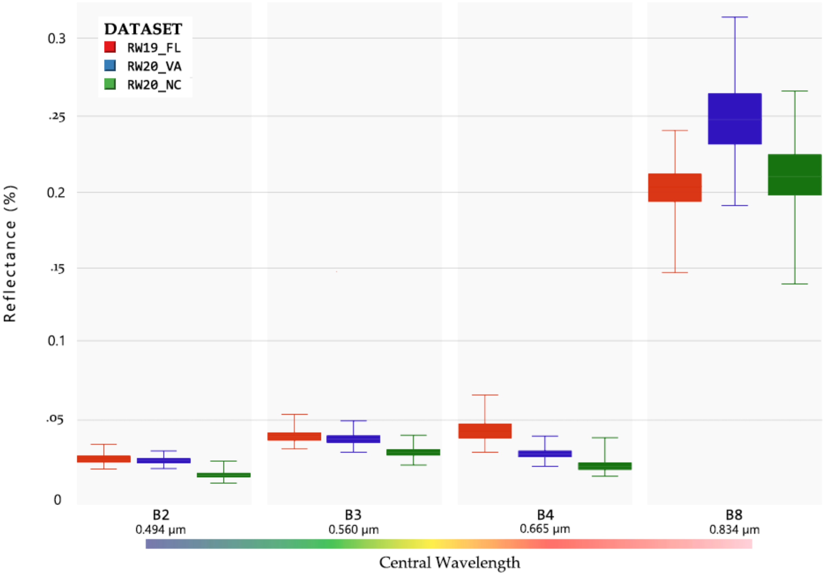
Only four of Sentinel-2’s Multispectral Instrument (MSI)’s 13 bands had a 10 m spatial resolution (Bands 2, 3, 4, and 8) and were used in this analysis (Table 4). The relative variance of surface reflectance for these four bands was explored between all plots for all 292 sites (Figure 2). Five common spectral indices were evaluated for performance in correlation with in situ observations of leaf area index measured with the LI-COR LAI-2200C instrument.
The implemented indices were: simple ratio (SR) index, normalized difference vegetation index (NDVI), soil adjusted vegetation index (SAVI), enhanced vegetation index (EVI), and a two-band enhanced vegetation index (EVI2).
Weighted and normalized means for each subsequent vegetation index were then extracted for all 292 field plots using the “extract” function from the R package raster. A simple linear regression was performed to select the best-performing vegetation index in linear correlation with the LAI-2200C field observations. The performance of each resulting model based on the spectral index was then tested by performing k-fold (n = 10) cross-validation using the caret package in R. This validation method evaluates model performance by randomly splitting the dataset into k-subsets (here, k = 10), reserving one subset and training the model against all the other subsets, then finally testing the model on the reserved subset. This process is repeated k-times, with the prediction error measured for each instance and averaged to ultimately serve as a performance metric [32].
Algorithm implementation, including but not limited to statistical analyses, radiometric conversion and spectral arithmetic, took place via the R programming language (R v.3.5.3) within the RStudio integrated development environment (v1.2.1335, Build 1379). See Table A1 for a complete list of R packages used.
2.3. Support Vector Machine Classification and Plot Segmentation
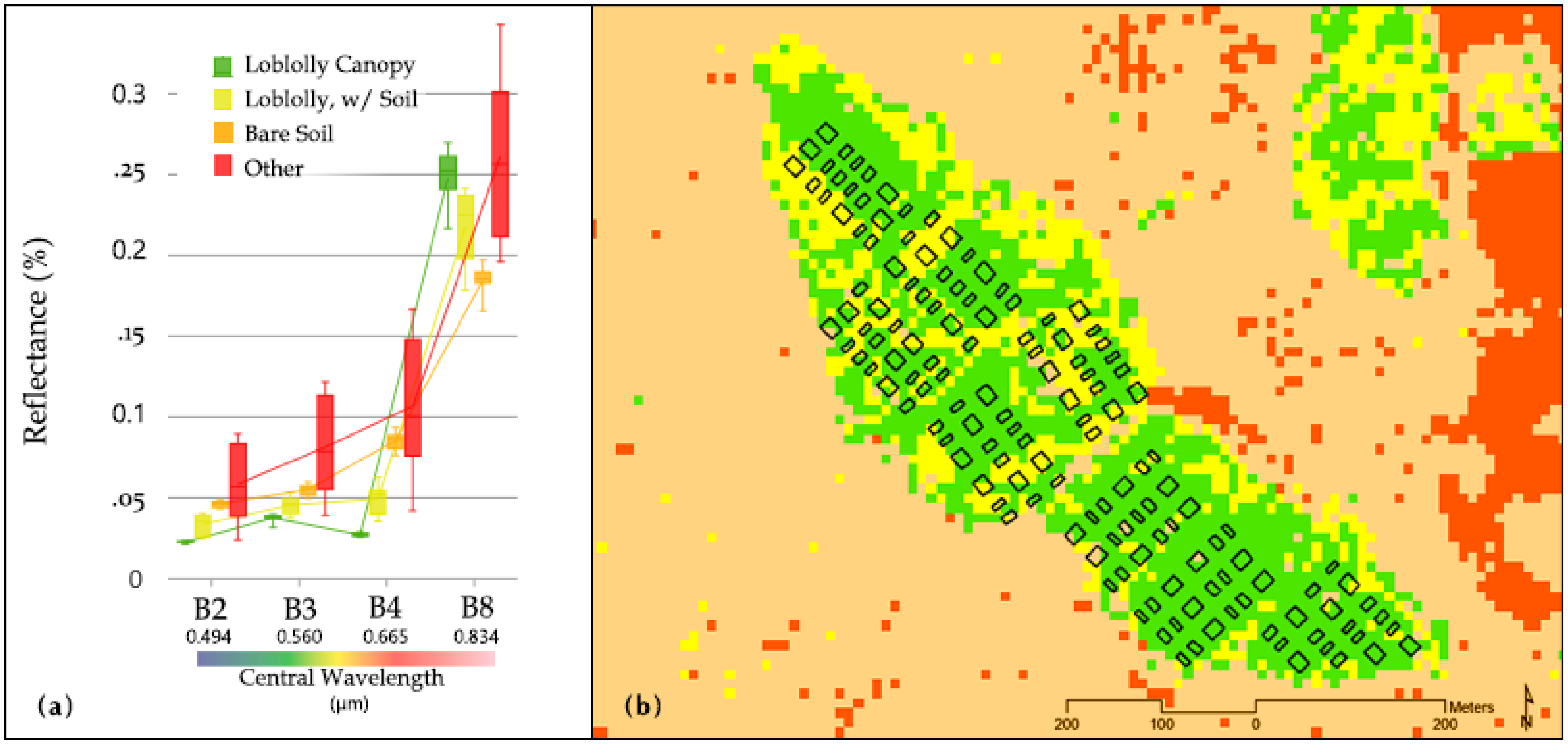
SVM classification was implemented using ArcGIS Pro (v2.4.2), and the following process was repeated independently for each of the three research sites. First, a classification schema was configured to subdivide training data classes according to categories of expectedly similar spectral categories: Loblolly Canopy; Loblolly w/Soil; Bare Soil; and Other. A spectral profile analysis was conducted across the entire Sentinel-2 scene prior to manually selecting training samples to fall into one of those four classes. Loblolly Canopy was defined as those grid cells most occupied by pure and unsaturated loblolly pine canopy. Loblolly w/Soil were regions within the loblolly plantation that certainly had their grid cell values gathered from loblolly pine canopy, but were also likely influenced by underlying soil reflectance and/or leaf litter. Bare Soil was attributed to samples collected where only dirt roads were found within the 10 m grid cell window. Other was composed of water, urban, and similarly undesired non-vegetative spectral attributes. Spectral profiles were used to guide each selection (Figure 3a). A minimum of 20 training sample polygons were established per class.
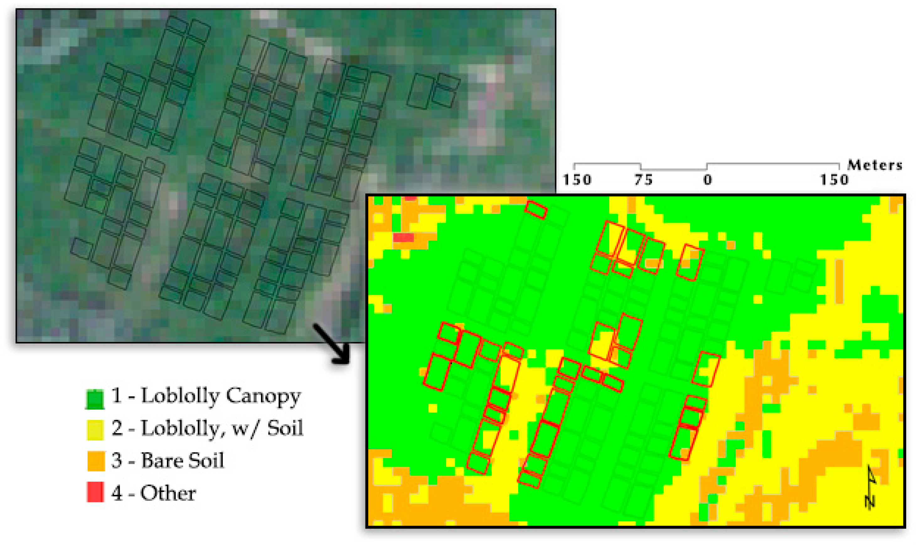
After the training dataset was delineated, the SVM classifier was run and the output images were analyzed and segmented (Figure 4). Plots whose boundaries covered the resulting SVM-determined class of Loblolly Canopy were always kept. Plots with the other three designated classes falling within their boundaries were systematically filtered, with Bare Soil and Other-occupied plot boundaries always being removed. Whether a plot occupied by the Loblolly w/Soil class was removed depended on the relative percentage (>50%) of the plot boundary covered by undesired spectra (Figure 4). Relative percentages of raster cell values within vector polygons can be retrieved using the “extract” function in the raster R package, specifically based on settings to the “weights” argument. For each polygon, a matrix with the cell values and the approximate fraction of each cell covered by the polygon is returned.
The resulting SVM-filtered dataset was then subjected to outlier detection based on boxplots of LAI-2200C values, whereby values were removed that fell above or below the 1.5 * interquartile range. After both of these processes were conducted, the completed dataset consisted of 218 plots (RW20-NC = 76; RW20-VA = 106; RW19-FL = 36). Distribution of LAI remained normal, with a range of 0.81 to 4.91. Weighted and normalized means were extracted for 218 plots based on five spectral indices. A linear regression model was fit such that in situ LAI was the dependent variable and the extracted spectral index mean was the independent variable.
2.4. Comparison to Industry Standard Models
Two industry standard models were compared with the best-fitting model produced in this analysis (Table 5). Landsat 7 and Landsat 8 imagery was obtained from the United States Geologic Survey EarthExplorer as analysis-ready datasets (ARDs). Datasets were filtered with cloud cover, cloud shadow cover, and snow and ice thresholds set to ≤6%. Imagery acquisition dates were 16 March 2018, 5 February 2018, and 20 January 2018 for RW19-FL, RW20-VA, and RW20-NC, respectively. The R package FPCLandsat was used to derive image products.
3. Results
3.1. LAI Model Formulation and Statistical Analysis
The best-performing spectral index prior to SVM and outlier removal was the simple ratio (SR) index (R2 = 0.56, RMSE = 0.63, coefficient estimate: 0.304, intercept: −0.025). See Table 6 for these results.
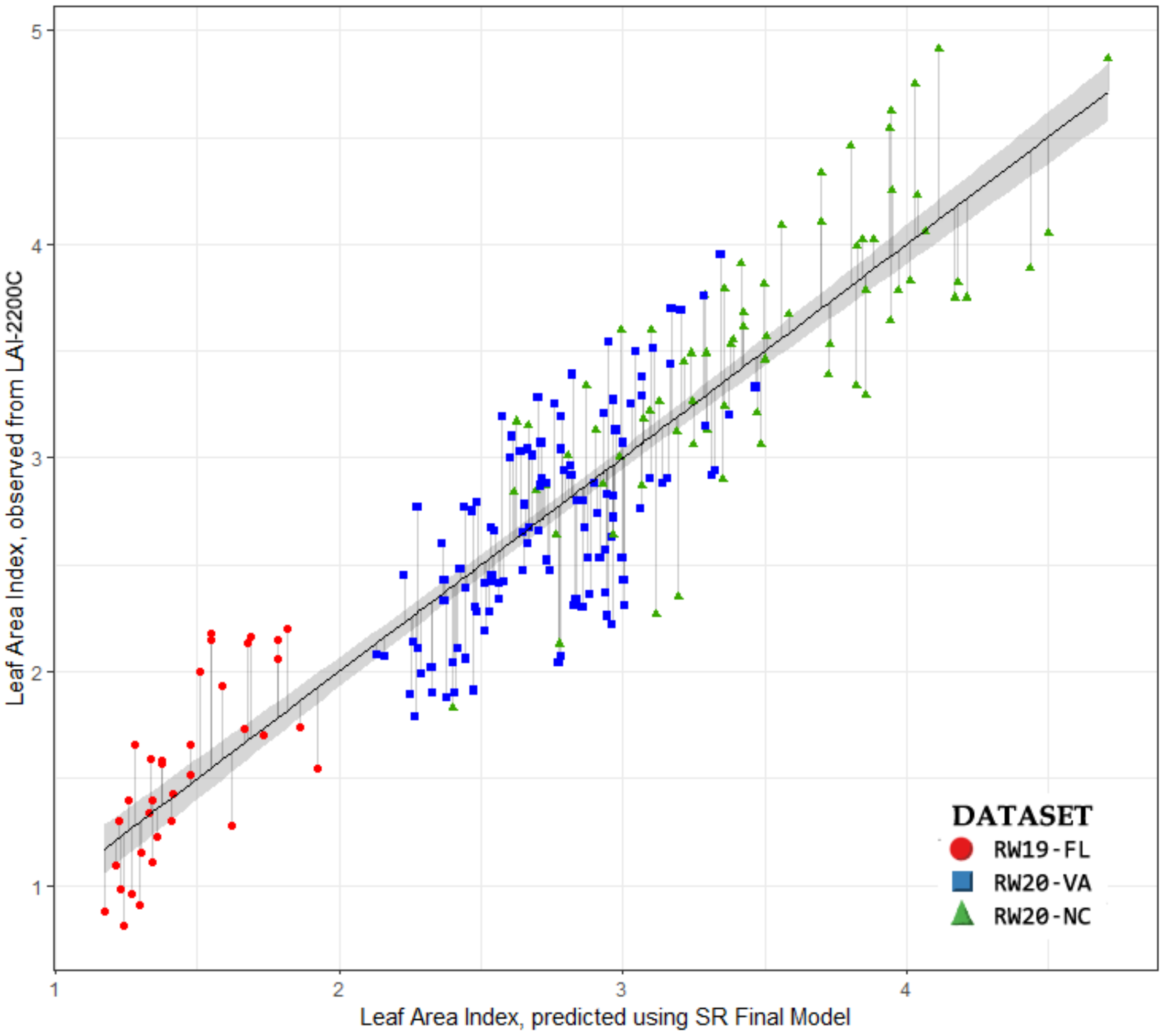
Post-SVM, the performance of each resulting spectral index model displayed the same ranking order as before SVM supervised classification and outlier removal, with SR performing best (Figure 5), followed by NDVI, SAVI, EVI, and EVI2. R2 and RMSE values improved throughout all index relationships.
SR and NDVI exhibited the strongest response (relative increase in R2 and decrease in RMSE) to SVM-supervised classification (Table 7). Akaike’s Information Criterion (AIC) values were reported, enabling comparison of model performance across multiple parameters.
The following equation was determined to be a generally applicable base model for loblolly pine plantations in the southeastern United States:
where SR is the simple ratio of near-infrared (NIR) and red bands (Band 8 and Band 4, respectively) calculated using Sentinel-2 Level-2A surface reflectance images.
3.2. Model Sensitivity Analysis to Imposed Treatments
A multiple linear regression model was used to evaluate changes in measured in situ LAIs due to imposed treatments (i.e., silviculture intensity, genetics, and planting density), with SR and plot-level treatments used as predictor variables as measured during the same season where the Sentinel-2 acquisition occurred (Table 8). SR and plot-level stand density at the time of the last field measurement were found to be significant. A linear relationship between predictor variables and in situ LAI was confirmed by plotting residuals (y-axis) against fitted values (x-axis). Residuals were normally distributed (confirmed by a standard Q-Q plot) and displayed homogeneity in variance (confirmed by a scale-location plot). Multicollinearity was assessed via a Pearson correlation matrix, with no high correlations (>0.7) between predictor variables being reported.
Other models, such as a multivariate regression model and a generalized linear mixed model (with varying matrices of fixed and random effects) were tried but discarded during the exploratory phase in favor of the multiple linear regression model.
Only the main effect of stand density improved model performance (R2 = 0.83 and RMSE = 0.35) over Equation (1). The relative effect of field-measured plot density was incorporated as a random effect in a linear mixed model using the lmer function of the lme4 package in R, and these results are displayed in Table 9. Ultimately, such a minor improvement ( + 0.02, RMSE–0.01, AIC-18) did not warrant amending the recommended equation where only the linear relationship between the in situ LAI and the Sentinel-2 simple ratio was used.
3.3. Comparison to Industry Standard Models
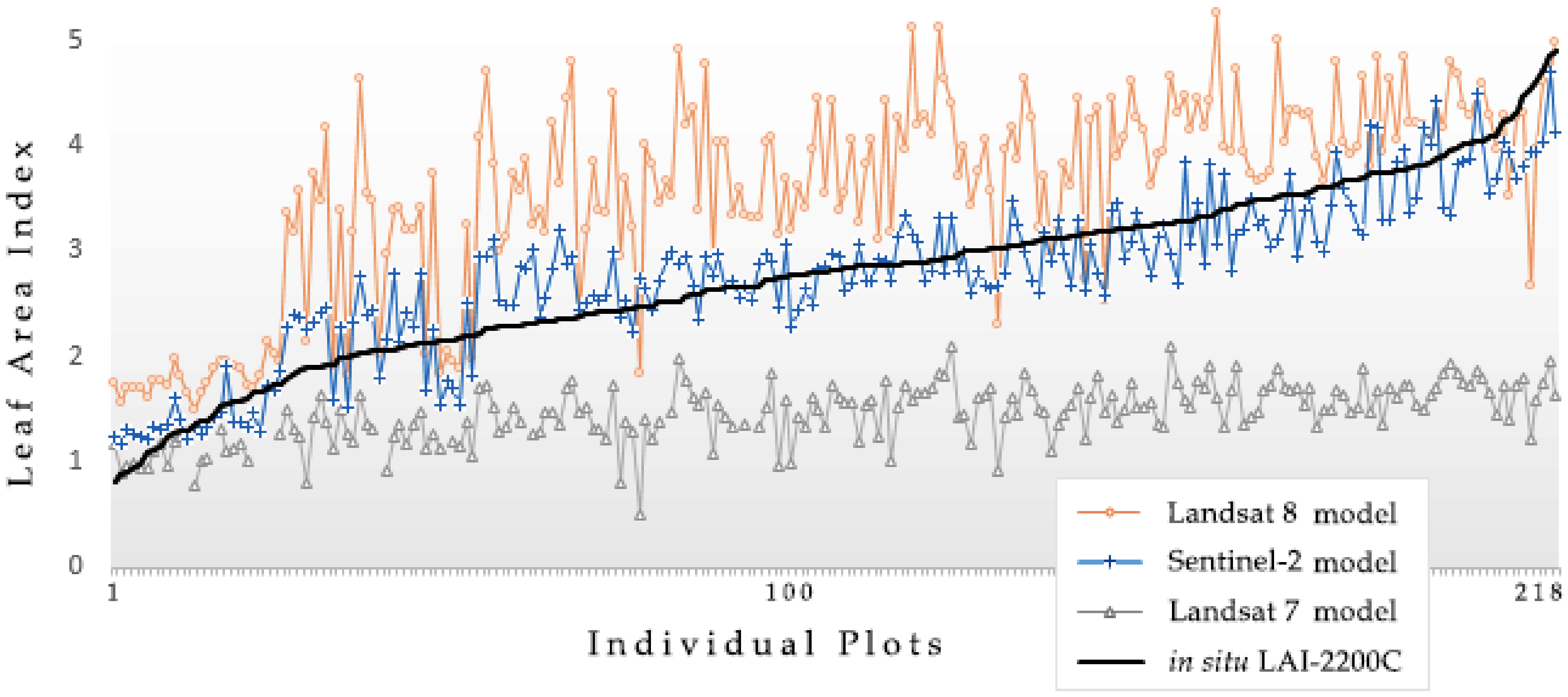
The best-fitting model produced in this analysis () proved similar to what Blinn et al 2019, observed in their model correlating Landsat 8s Operational Land Imager and Thermal Infrared Sensor (OLI-TIRS) with LAI-2200C values [9]. Comparing the Landsat 8 model to our Sentinel-2 model showed that the Landsat 8 model generally over-predicted field LAI (Figure 6). This over-prediction was probably most closely associated with the 30 m spatial resolution restrictions of the Landsat 8 OLI-TIRS, thereby permitting estimates based on fewer raster cells per measurement plot boundary than the Sentinel-2 MSI. A previous industry standard model based off of the simple ratio between near-infrared/red bands and top-of-atmosphere reflectance derived from Landsat 7s Enhanced Thematic Mapper (ETM) was also included in this direct comparison [7]. The Landsat 7 model underpredicted at all intervals except the very lowest end of the LAI spectrum. This underprediction is likely because the Landsat 7 model was based on top-of-atmosphere reflectance, thereby not accounting for atmospheric interference by clouds, aerosols, and other potential contributions. Also, the Landsat 7 data were simultaneously based off fewer in situ LAI values (n = 12) at a single site in the Sandhills of North Carolina.
4. Discussion
4.1. Model Performance and Interpretations
Our model performed well across three sites under multiple conditions typical of managed loblolly pine, but performance has yet to be gauged across even broader geographic ranges, under different site and management conditions. Robustness of the training dataset was determined by the range of variability at site-, stand-, and individual-tree-level perspectives. Loblolly pine displays variance in its structural development—specifically the formation of its crown and related foliar density—associated with intrinsic site attributes largely tied to the underlying soil [38]. For instance, soil drainage class and subsoil texture have been demonstrated to have a marked effect on growth efficiency, which is a metric gauging the relationship between volume production and leaf area index [39]. Growth efficiency (the efficiency with which an individual tree makes use of site resources to produce stem biomass) as well as LAI have been considered across sites with variability such as these before, with responses to silviculture being most apparent on nutrient-deficient, poorly drained sites like RW20-NC [40]. Albaugh et al. (2019) specifically explored the growth efficiency and crown dynamics of RW20 sites, concluding that unexplored site variables are causing the large degree of variance in crown architecture, crown leaf area distribution, and individual tree growth efficiency between individual sites [41]. The ideal training dataset would cover as broad of a geographic range as possible to account for variety in loblolly pine’s native range. This is because a change in one’s geographic location results in a shift in site resource availability, which is a function of several things—nutrient supplying power, amount of rainfall, temperature, and so on. While the training dataset used in our analysis did not stretch across loblolly pine’s entire native range, to our knowledge no similar published work has incorporated a dataset as geographically extensive or measuring a greater number of in situ plots than the dataset applied here.
As with any model, minor deviations can be expected in sites that are dissimilar (in terms of geographic region, soil, stand composition, etc.) from those used for this analysis. Likewise, when making inferences for values outside of those measured during model construction, one should expect a loss of model accuracy. For instance, the model recommended here did not perform well at LAI values below 1, because very few in situ LAI values were measured below 1. Lower density plots (≤618 trees per hectare), which had a lower stand-level LAI, were marginally overpredicted (Table 9) at a scale of approximately 0.2 LAI. All other predicted LAI-by-density ranges displayed homoscedasticity, implying that the model was relatively stable across the remaining density spectrum (~621–2225 trees per hectare).
The use of SVM-supervised classification to improve the relationship between Sentinel-2 and LAI-2200C proved useful in removing undesired spectral values, but the resulting model did not differ greatly from the relationship modeled prior to SVM and outlier removal. Supervised classification in this situation was only used to attempt to improve the prediction accuracy of the model itself. The aerial, top-down perspective, combined with the electromagnetic sensitivity of a satellite instrument sensor such as the MSI from Sentinel-2, is likely a more consistent metric of stand variance across time and space than the LAI-2200C instrument alone. Supervised classifiers are inherently subject to user error (the supervised element), though this common bias was sought to be removed through single-pixel selection paired alongside spectra profiles to best select those classes exhibiting reflectance characteristics of their delineation.
Based on our analysis, a reasonable range of accuracy in estimating LAI at a 10 m spatial resolution is ±0.4 (Table 7). A positive trait about the simple ratio is that it is just as its name implies, a simple relationship between the NIR and red wavelengths. It becomes possible to explain some of the variance one picks up from such a minimalized band relationship, but one is still likely to see variance in estimated LAI that may or may not be explainable. Lower density stands will have more openings in their canopy, thus exposing the resulting analysis based on reflectance spectra to confounding variables such as soil, leaf litter, moisture and snow reflectance, and more.
4.2. Future Research Directions
SVM classification proved successful in improving the linear model developed between SR and LAI-2200C, but the relative improvement over the raw relationship between the two was low (based solely on changes in coefficient and intercept estimates). Indicators of fit ( and RMSE) were improved when examining management use cases, but whether one would observe these levels of accuracy from a standard operational perspective is still unknown. Improvements to the machine learning aspect of this analysis could certainly be made, such as further incorporating more data points, and using recently introduced algorithms have been beneficial to specific-use cases such as scene filtering among site heterogeneity [42]. Inclusion of datasets with individual tree metrics and underlying soil characteristics may lead to a better estimation of leaf area trends across space and time. Datasets of higher spatial resolutions would also likely lead to advances in projecting growth efficiency and similar metrics across sites, such as with LiDAR datasets.
Consideration of other bands available in the Sentinel-2 MSI becomes more appealing when datasets are robust like those used in this analysis, though they exhibit coarser spatial resolutions than those considered in this work. It is logical to consider plot-level interactions from a perspective of increased hyperspectral range, specifically in the red-edge spectrum afforded by Sentinel-2 bands 4, 5, and 6. Following this now well-researched trend that approximately a third of the simple ratio between near-infrared and red bands is equal to in situ loblolly pine LAI, additional variances in LAI may be captured through a more detailed, finer-scaled inspection of remote sensing imagery paired with detailed site metrics. Few researchers have considered the use of machine learning and newer computer vision technology to improve correlations between dependent variables (e.g., nitrogen or chlorophyll content) and their reflectance observed on red-edge wavelengths [43]. Especially since it has been observed that Sentinel-2 red edge bands can improve predictions of chlorophyll and nitrogen content [44,45], it appears worthwhile to consider these other bands for future use in similar applications. Incorporation of these spectral bands into an operational forest management application have yet to be explored.
5. Conclusions
The resulting equation (LAI = 0.310SR − 0.098) displayed good performance at estimating LAI at a 10 m spatial resolution for loblolly pine. We reported a statistically significant interaction between stand density (≤618 trees per hectare) and model performance, though the implications of a density interaction was deemed operationally insignificant to warrant adjusting the model. Support vector machine-supervised classification was successfully used to distinguish plots whose weighted mean leaf area index value was primarily derived by the association between LAI-2200C plant canopy analyzer and Sentinel-2 MSI, removing plots whose spectral range saturated beyond training classes established for this relationship. The SVM-aided model exhibited relatively negligible variance from the model based on the same spectral index—simple ratio of near-infrared and red bands—prior to SVM classification and outlier removal. The 10 m spatial resolution afforded by Sentinel-2 provides for spatially robust biophysical site metrics like LAI to be generated and used for high-fidelity forest management. As site variability across the landscape becomes more precisely gauged, an opportunity to base remote sensing models on strategically placed field locations exists that could better model dynamic and complex ecological processes across a broader landscape. The relationship between remote sensing systems and biophysical indicators of forest ecosystem status, such as leaf area index, should continue to be explored so long as improvements in modeling these relationships exist.
Author Contributions
Conceptualization, R.L.C. and C.W.C.; methodology, J.M.G. and C.W.C; software, C.W.C.; validation, C.W.C., R.L.C., J.M.G., and T.J.A.; formal analysis, C.W.C.; investigation, C.W.C. and R.L.C.; resources, C.W.C., R.L.C., and T.J.A.; data curation, T.J.A. and C.W.C.; writing—original draft preparation, C.W.C.; writing—review and editing, R.L.C., J.M.G., T.J.A., and C.W.C.; visualization, C.W.C.; supervision, R.L.C. and J.M.G.; project administration, R.L.C.; funding acquisition, R.L.C. All authors have read and agree to the published version of the manuscript.
Funding
Support for this research was provided by members of the Forest Productivity Cooperative and by NC State University’s Department of Forestry and Environmental Resources.
Acknowledgments
Acknowledgment is given to past and present members and staff of the Forest Productivity Cooperative. We gratefully acknowledge the support provided by the National Science Foundation Center for Advanced Forest Systems, the Department of Forestry and Environmental Resources at North Carolina State University, and the Department of Forest Resources and Environmental Conservation at Virginia Tech. Funding for this work was provided in part by the Virginia Agricultural Experiment Station and the McIntire-Stennis Program of the National Institute of Food and Agriculture, U.S. Department of Agriculture.
Conflicts of Interest
The authors declare no conflict of interest.
Appendix A
Figure A1.
Comparison between the minimum spatial resolutions of Sentinel-2 and Landsat 8. Shown in the same selected subset of field plots from RW20-NC with the 10 m grid cells of Sentinel-2 on the top and the 30 m grid cells of Landsat 8 on the bottom.
Figure A1.
Comparison between the minimum spatial resolutions of Sentinel-2 and Landsat 8. Shown in the same selected subset of field plots from RW20-NC with the 10 m grid cells of Sentinel-2 on the top and the 30 m grid cells of Landsat 8 on the bottom.

Appendix B

Table A1.
Summary of primary R packages used throughout this work.
| Package | Version | Author(s) | CRAN URL |
|---|---|---|---|
| tidyverse | 1.3.0 | Hadley Wickham | https://cran.r-project.org/web/packages/tidyverse/index.html |
| caret | 6.0 | Max Kuhn et. al. | https://cran.r-project.org/web/packages/caret/index.html |
| ggplot2 | 3.2.1 | Hadley Wickham et. al. | https://cran.r-project.org/web/packages/ggplot2/index.html |
| lme4 | 1.1-21 | Douglas Bates et. al. | https://cran.r-project.org/web/packages/lme4/index.html |
| rgdal | 1.4-8 | Roger Bivand et. al. | https://cran.r-project.org/web/packages/rgdal/index.html |
| raster | 3.0-7 | Robert J. Hijmans et. al. | https://cran.r-project.org/web/packages/raster/index.html |
| sf | 0.8-0 | Edzer Pebesma et. al. | https://cran.r-project.org/web/packages/sf/index.html |
References
- Prestemon, J.P.; Abt, R.C. Timber products supply and demand. In The Southern Forest Resource Assessment; Technical Report No. GTR-SRS-53; USDA-Forest Service, Southern Research Station: Asheville, NC, USA, 2002; pp. 299–325. Available online: https://www.fs.usda.gov/treesearch/pubs/42386 (accessed on 18 December 2019).
- Fox, T.; Allen, H.; Albaugh, T. Tree nutrition and forest fertilization of pine plantations in the southern United States. South. J. Appl. For. 2007, 31, 5–11. [Google Scholar] [CrossRef] [Green Version]
- Allen, H.L. Silvicultural treatments to enhance productivity. In The Forests Handbook: Applying Forest Science for Sustainable Management; Blackwell Science: Oxford, UK, 2001; Volume 2, pp. 129–139. [Google Scholar]
- Will, R.E.; Narahari, N.V.; Shiver, B.D.; Teskey, R.O. Effects of planting density on canopy dynamics and stem growth for intensively managed loblolly pine stands. For. Ecol. Manag. 2005, 205, 29–41. [Google Scholar] [CrossRef]
- Ke, Y.; Im, J.; Lee, J.; Gong, H.; Ryu, Y. Characteristics of Landsat 8 OLI-derived NDVI by comparison with multiple satellite sensors and in-situ observations. Remote Sens. Environ. 2015, 164, 298–313. [Google Scholar] [CrossRef]
- Pflugmacher, D.; Cohen, W.B.; Kennedy, R.E.; Yang, Z. Using Landsat-derived disturbance and recovery history and lidar to map forest biomass dynamics. Remote Sens. Environ. 2014, 151, 124–137. [Google Scholar] [CrossRef]
- Flores, F.J.; Allen, H.L.; Cheshire, H.M.; Davis, J.M.; Fuentes, M.; Kelting, D. Using multispectral satellite imagery to estimate leaf area and response to silvicultural treatments in loblolly pine stands. Can. J. For. Res. 2006, 36, 1587–1596. [Google Scholar] [CrossRef] [Green Version]
- Franklin, S.E.; Lavigne, M.B.; Deuling, M.J.; Wulder, M.A.; Hunt, E.R., Jr. Estimation of forest leaf area index using remote sensing and GIS data for modelling net primary production. Int. J. Remote Sens. 1997, 18, 3459–3471. [Google Scholar] [CrossRef]
- Blinn, C.E.; House, M.N.; Wynne, R.H.; Thomas, V.A.; Fox, T.R.; Sumnall, M. Landsat 8 based leaf area index estimation in loblolly pine plantations. Forests 2019, 10, 222. [Google Scholar] [CrossRef] [Green Version]
- Drusch, M.; Del Bello, U.; Carlier, S.; Colin, O.; Fernandez, V.; Gascon, F.; Hoersch, B.; Isola, C.; Laberinti, P.; Martimort, P.; et al. Sentinel-2: ESA’s optical high-resolution mission for GMES operational services. Remote Sens. Environ. 2012, 120, 25–36. [Google Scholar] [CrossRef]
- Meyer, L.H.; Heurich, M.; Beudert, B.; Premier, J.; Pflugmacher, D. Comparison of Landsat-8 and Sentinel-2 data for estimation of leaf area index in temperate forests. Remote Sens. 2019, 11, 1160. [Google Scholar] [CrossRef] [Green Version]
- Welles, J.M. Some indirect methods of estimating canopy structure. Remote Sens. Rev. 1990, 5, 31–43. [Google Scholar] [CrossRef]
- Chen, J.M. Remote sensing of leaf area index and clumping index. In Comprehensive Remote Sensing; Elsevier: Amsterdam, The Netherlands, 2018; Volume 3, pp. 53–77. [Google Scholar] [CrossRef]
- Ryu, Y.; Nilson, T.; Kobayashi, H.; Sonnentag, O.; Law, B.E.; Baldocchi, D.D. On the correct estimation of effective leaf area index: Does it reveal information on clumping effects? Agric. For. Meteorol. 2010, 150, 463–472. [Google Scholar] [CrossRef]
- Jonckheere, I.; Fleck, S.; Nackaerts, K.; Muys, B.; Coppin, P.; Weiss, M. Methods for leaf area index determination. Part I: Theories, techniques and instruments. Agric. For. Meteorol. 2004, 121, 19–35. [Google Scholar] [CrossRef]
- Asner, G.P. Biophysical and biochemical sources of variability in canopy reflectance. Remote Sens. Environ. 1998, 64, 234–253. [Google Scholar] [CrossRef]
- Rautiainen, M.; Lukeš, P.; Homolova, L.; Hovi, A.; Pisek, J.; Mõttus, M. Spectral properties of coniferous forests: A review of in situ and laboratory measurements. Remote Sens. 2018, 10, 207. [Google Scholar] [CrossRef] [Green Version]
- Wang, R.; Chen, J.M.; Liu, Z.; Arain, A. Evaluation of seasonal variations of remotely sensed leaf area index over five evergreen coniferous forests. ISPRS J. Photogramm. Remote Sens. 2017, 130, 187–201. [Google Scholar] [CrossRef]
- Pisek, J.; Chen, J.M.; Alikas, K.; Deng, F. Impacts of including forest understory brightness and foliage clumping information from multiangular measurements on leaf area index mapping over North America. J. Geophys. Res. Biogeosci. 2010, 115(G3). [Google Scholar] [CrossRef] [Green Version]
- Mountrakis, G.; Im, J.; Ogole, C. Support vector machines in remote sensing: A review. ISPRS J. Photogramm. Remote Sens. 2011, 66, 247–259. [Google Scholar] [CrossRef]
- Hänsch, R.; Schulz, K.; Sörgel, U. Machine learning methods for remote sensing applications: An overview. In Proceedings of the SPIE Remote Sensing, Berlin, Germany, 10–13 September 2018; Volume 10790. [Google Scholar] [CrossRef]
- Signoroni, A.; Savardi, M.; Baronio, A.; Benini, S. Deep learning meets hyperspectral image analysis: A multidisciplinary review. J. Imaging 2019, 5, 52. [Google Scholar] [CrossRef] [Green Version]
- Ma, L.; Liu, Y.; Zhang, X.; Ye, Y.; Yin, G.; Johnson, B.A. Deep learning in remote sensing applications: A meta-analysis and review. ISPRS J. Photogramm. Remote Sens. 2019, 152, 166–177. [Google Scholar] [CrossRef]
- Fassnacht, F.E.; Latifi, H.; Ghosh, A.; Joshi, P.K.; Koch, B. Assessing the potential of hyperspectral imagery to map bark beetle-induced tree mortality. Remote Sens. Environ. 2014, 140, 533–548. [Google Scholar] [CrossRef]
- Kamilaris, A.; Prenafeta-Boldú, F.X. Deep learning in agriculture: A survey. Comput. Electron. Agric. 2018, 147, 70–90. [Google Scholar] [CrossRef] [Green Version]
- Zermas, D.; Teng, D.; Stanitsas, P.; Bazakos, M.; Kaiser, D.; Morellas, V.; Mulla, D.; Papanikolopoulos, N. Automation solutions for the evaluation of plant health in corn fields. In Proceedings of the 2015 IEEE/RSJ International Conference on Intelligent Robots and Systems (IROS), Hamburg, Germany, 28 September–2 October 2015; pp. 6521–6527. [Google Scholar] [CrossRef]
- Albaugh, T.J.; Fox, T.R.; Maier, C.A.; Campoe, O.C.; Rubilar, R.A.; Cook, R.L.; Raymond, J.E.; Alvares, C.A.; Stape, J.L. A common garden experiment examining light use efficiency and heat sum to explain growth differences in native and exotic Pinus taeda. For. Ecol. Manag. 2018, 425, 35–44. [Google Scholar] [CrossRef] [Green Version]
- Albaugh, T.J.; Fox, T.R.; Rubilar, R.A.; Cook, R.L.; Amateis, R.L.; Burkhart, H.E. Post-thinning density and fertilization affect Pinus taeda stand and individual tree growth. For. Ecol. Manag. 2017, 396, 207–216. [Google Scholar] [CrossRef] [Green Version]
- Garrigues, S.; Lacaze, R.; Baret, F.J.T.M.; Morisette, J.T.; Weiss, M.; Nickeson, J.E.; Fernandes, R.; Plummer, S.; Shabanov, N.V.; Myneni, R.B.; et al. Validation and intercomparison of global leaf area index products derived from remote sensing data. J. Geophys. Res. 2008, 113. [Google Scholar] [CrossRef]
- Welles, J.M.; Norman, J.M. Instrument for indirect measurement of canopy architecture. Agron. J. 1991, 83, 818–825. [Google Scholar] [CrossRef]
- Fang, H.; Liang, S. Leaf area index models. Encycl. Ecol. 2008, 2139–2148. [Google Scholar] [CrossRef]
- James, G.; Witten, D.; Hastie, T.; Tibshirani, R. An Introduction to Statistical Learning: With Applications in R; Springer: New York, NY, USA, 2014. [Google Scholar]
- Birth, G.S.; McVey, G.R. Measuring the color of growing turf with a reflectance spectrophotometer 1. Agron. J. 1968, 60, 640–643. [Google Scholar] [CrossRef]
- Rouse, J.W., Jr.; Haas, R.H.; Schell, J.A.; Deering, D.W. Monitoring vegetation systems in the Great Plains with ERTS. In Third Earth Resources Technology Satellite—1 Symposium; NASA: Washington, DC, USA, 1974; Volume I. [Google Scholar]
- Huete, A.R. A soil-adjusted vegetation index (SAVI). Remote Sens. Environ. 1988, 25, 295–309. [Google Scholar] [CrossRef]
- Liu, H.Q.; Huete, A. A feedback based modification of the NDVI to minimize canopy background and atmospheric noise. IEEE Trans. Geosci. Remote Sens. 1995, 33, 457–465. [Google Scholar] [CrossRef]
- Jiang, Z.; Huete, A.R.; Didan, K.; Miura, T. Development of a two-band enhanced vegetation index without a blue band. Remote Sens. Environ. 2008, 112, 3833–3845. [Google Scholar] [CrossRef]
- Sampson, D.A.; Allen, H.L. Regional influences of soil available water-holding capacity and climate, and leaf area index on simulated loblolly pine productivity. For. Ecol. Manag. 1999, 124, 1–12. [Google Scholar] [CrossRef]
- Rojas, J.C. Factors Influencing Responses of Loblolly Pine Stands to Fertilization. Ph.D. Thesis, North Carolina State University, Raleigh, NC, USA, August 2005. [Google Scholar]
- Albaugh, T.J.; Allen, H.L.; Zutter, B.R.; Quicke, H.E. Vegetation control and fertilization in midrotation Pinus taeda stands in the southeastern United States. Ann. For. Sci. 2003, 60, 619–624. [Google Scholar] [CrossRef] [Green Version]
- Albaugh, T.J.; Maier, C.A.; Campoe, O.C.; Yáñez, M.A.; Carbaugh, E.D.; Carter, D.R.; Cook, R.L.; Rubilar, R.A.; Fox, T.R. Crown architecture, crown leaf area distribution, and individual tree growth efficiency vary across site, genetic entry, and planting density. Trees 2019, 34, 73–88. [Google Scholar] [CrossRef]
- Heydari, S.S.; Mountrakis, G. Effect of classifier selection, reference sample size, reference class distribution and scene heterogeneity in per-pixel classification accuracy using 26 Landsat sites. Remote Sens. Environ. 2018, 204, 648–658. [Google Scholar] [CrossRef]
- Watt, M.S.; Pearse, G.D.; Dash, J.P.; Melia, N.; Leonardo, E.M.C. Application of remote sensing technologies to identify impacts of nutritional deficiencies on forests. ISPRS J. Photogramm. Remote Sens. 2019, 149, 226–241. [Google Scholar] [CrossRef]
- Xie, Q.; Dash, J.; Huete, A.; Jiang, A.; Yin, G.; Ding, Y.; Peng, D.; Hall, C.C.; Brown, L.; Shi, Y.; et al. Retrieval of crop biophysical parameters from Sentinel-2 remote sensing imagery. Int. J. Appl. Earth Obs. Geoinf. 2019, 80, 187–195. [Google Scholar] [CrossRef]
- Cai, Y.; Guan, K.; Nafziger, E.; Chowdhary, G.; Peng, B.; Jin, Z.; Wang, S.; Wang, S. Detecting in-season crop nitrogen stress of corn for field trials using UAV-and CubeSat-based multispectral sensing. IEEE J. Sel. Top. Appl. Earth Obs. Remote Sens. 2019, 12, 5153–5166. [Google Scholar] [CrossRef]
Figure 1.
Location map of the three sites used for field validation in this study. Latitude and longitude coordinates indicate the approximate center location(s) for each site.
Figure 1.
Location map of the three sites used for field validation in this study. Latitude and longitude coordinates indicate the approximate center location(s) for each site.

Figure 2.
Boxplots of Sentinel-2 band reflectance values showing the relative variance of surface reflectance observed between all plots for all sites used in this analysis. Number of total plots included = 292. Only those Sentinel-2 MSI bands with a spatial resolution of 10 m were used. B2 = Blue; B3 = Green; B4 = Red; B8 = NIR.

Figure 3.
Shown here are (a) reflectance spectra for individual training samples, displaying the relative range in reflectance for each training sample class, and (b) the RW20-VA raster output using the support vector machine (SVM)-supervised classification based on the four classes.
Figure 3.
Shown here are (a) reflectance spectra for individual training samples, displaying the relative range in reflectance for each training sample class, and (b) the RW20-VA raster output using the support vector machine (SVM)-supervised classification based on the four classes.

Figure 4.
RW20-NC delineated using support vector machine-supervised classification, then having plots filtered (shown with red boundary) where soil or leaf litter reflectance saturation occurred.
Figure 4.
RW20-NC delineated using support vector machine-supervised classification, then having plots filtered (shown with red boundary) where soil or leaf litter reflectance saturation occurred.

Figure 5.
Simple Ratio model performance, post-SVM and outlier removal. Model-estimated LAI values are on the x-axis and field-observed LAI-2200C values are on the y-axis. Residuals are visualized by lines drawn from the primary linear regression line. A 95% confidence interval envelops the regression line in gray.

Figure 6.
Comparing the model produced in this article (Sentinel-2) against two prior industry standard models (using Landsat 7 and Landsat 8) [7,9]. Null data for the Landsat 7 model results from Enhanced Thematic Mapper (ETM) scan line corrector failure.

Table 1.
Silvicultural and generalized management history of datasets used in analysis.
| Dataset ID | Year Planted (Tree Age) | Planting Density (Trees per Hectare) | Silvicultural Activities | Genetics |
|---|---|---|---|---|
| RW19-FL | 2000 (18) | 250, 500, 750, 1235, >1235 | Thinning; Fertilization | Open Pollinated |
| RW20-VA | 2009 (9) | 618, 1235, 1835 | Competition Control; Fertilization | Mass-control Pollinated; Open Pollinated; 4 Clones |
| RW20-NC | 2009 (9) | 618, 1235, 1835 | Competition Control; Fertilization | Mass-control Pollinated; Open Pollinated; 4 Clones |
Table 2.
Soil and geological characteristics of sites used in this study.
| Dataset ID | Soil Texture | Soil Drainage | USDA Soil Series | Underlying Geology (Parent Material) |
|---|---|---|---|---|
| RW19-FL | Sand; sandy loam (spodic) | Somewhat to Very Poorly Drained | Chaires; Goldhead; Albany | Atlantic Flatwoods, upper terrace (beach sand; clay; mud) |
| RW20-VA | Fine loamy; Clayey | Well Drained | Fairview; Braddock | Schist; Phyllite |
| RW20-NC | Fine loamy | Poorly Drained | Rains | Alluvium; loess; sand |
Table 3.
General location and collection overview of datasets used in analysis.
| Dataset ID (County) | Date of Field Observation | Date of Sentinel-2 Acquisition | Days Variance | LAI2200C Range | Number of Plots |
|---|---|---|---|---|---|
| RW19-FL (Nassau) | 5 Mar 2018 | 15 Mar 2018 | +10 | 0.81–2.36 | 40 |
| RW20-VA (Patrick) | 31 Jan 2018 | 8 Feb 2018 | +9 | 0.89–5.09 | 144 |
| RW20-NC (Bladen) | 24 Jan 2018 | 24 Jan 2018 | 0 | 0.92–5.64 | 108 |
Table 4.
Wavelength specifications and bandwidths for Sentinel-2A Multispectral Instrument (MSI) bands that had a spatial resolution of 10 m.
Table 4.
Wavelength specifications and bandwidths for Sentinel-2A Multispectral Instrument (MSI) bands that had a spatial resolution of 10 m.
| Band Number | Description | Central Wavelength (μm) | Wavelength (Min–Max) | Bandwidth |
|---|---|---|---|---|
| 2 | Blue | 0.494 | 0.439–0.535 | 0.096 |
| 3 | Green | 0.560 | 0.537–0.582 | 0.045 |
| 4 | Red | 0.665 | 0.646–0.685 | 0.039 |
| 8 | NIR | 0.834 | 0.767–0.908 | 0.141 |
Table 5.
Industry standard models used for comparison against the Sentinel-2 model. LAI = leaf area index.
Table 5.
Industry standard models used for comparison against the Sentinel-2 model. LAI = leaf area index.
| Model | Equation |
|---|---|
| Landsat 7 Model [7] | |
| Landsat 8 Model [9] |
Table 6.
Results of initial exploratory linear regression for five spectral indices across all 292 plots (prior to support vector machine supervised classification and outlier removal). Terms represent spectral indices: simple ratio (SR) index, normalized difference vegetation index (NDVI), soil adjusted vegetation index (SAVI), enhanced vegetation index (EVI), and a two-band enhanced vegetation index (EVI2).
| Term | MSI Equation | R2 | RMSE |
|---|---|---|---|
| SR [33] | 0.56 | 0.63 | |
| NDVI [34] | 0.49 | 0.67 | |
| SAVI [35] | 0.15 | 0.87 | |
| EVI [36] | 0.10 | 0.89 | |
| EVI2 [37] | 0.10 | 0.89 |
Table 7.
Post-SVM and outlier removal results of k-fold (n = 10) cross-validation for the five spectral vegetation indices utilized in simple linear regression equations. Bold indicates best-fitting interaction. AIC = Akaike’s Information Criterion.
Table 7.
Post-SVM and outlier removal results of k-fold (n = 10) cross-validation for the five spectral vegetation indices utilized in simple linear regression equations. Bold indicates best-fitting interaction. AIC = Akaike’s Information Criterion.
| Term | Root Mean Square Error (RMSE) | Mean Absolute Error (MAE) | AIC | |
|---|---|---|---|---|
| SR | 0.81 | 0.36 | 0.30 | 187 |
| NDVI | 0.72 | 0.43 | 0.35 | 262 |
| SAVI | 0.27 | 0.72 | 0.60 | 481 |
| EVI | 0.19 | 0.76 | 0.63 | 505 |
| EVI2 | 0.19 | 0.76 | 0.63 | 504 |
Table 8.
A multiple linear regression model evaluated in situ LAI, with SR and plot-level factors used as predictor variables. Adj. = 0.827. RMSE = 0.347. AIC = 169. Bold indicates significance based on an alpha level of 0.005.
Table 8.
A multiple linear regression model evaluated in situ LAI, with SR and plot-level factors used as predictor variables. Adj. = 0.827. RMSE = 0.347. AIC = 169. Bold indicates significance based on an alpha level of 0.005.
| Table | Estimate | Std. Error | T-Value | p-Value |
|---|---|---|---|---|
| SR | 0.3075 | 0.0122 | 25.152 | <0.0001 |
| Silv. Intensity 1 | 0.0534 | 0.0507 | 1.054 | 0.2932 |
| Density | 0.0005 | 0.0001 | 4.084 | <0.0001 |
| Genetics | 0.0226 | 0.01447 | 1.564 | 0.1192 |
1 For RW19-FL, silviculture intensity implies fertilized vs unfertilized after thinning. In RW20-NC and RW20-FL, silvicultural intensity denotes operational silviculture vs intensive silviculture.
Table 9.
Statistical summary of change in slope relative to field-measured plot density (trees per hectare), as a random effect, incorporated into a linear mixed model (response variable = in situ LAI; fixed effect = SR) at the time of Sentinel-2 image acquisition.
Table 9.
Statistical summary of change in slope relative to field-measured plot density (trees per hectare), as a random effect, incorporated into a linear mixed model (response variable = in situ LAI; fixed effect = SR) at the time of Sentinel-2 image acquisition.
| Density (Trees per Hectare) | Intercept | Simple Ratio Coefficient |
|---|---|---|
| ≤250 | −0.139 | 0.310 |
| 251–618 | −0.164 | 0.310 |
| 619–750 | −0.070 | 0.310 |
| 751–1000 | −0.053 | 0.310 |
| 1001–1250 | −0.006 | 0.310 |
| 1251–1500 | −0.050 | 0.310 |
| 1501–1750 | −0.023 | 0.310 |
| 1751–2225 | −0.047 | 0.310 |
© 2020 by the authors. Licensee MDPI, Basel, Switzerland. This article is an open access article distributed under the terms and conditions of the Creative Commons Attribution (CC BY) license (http://creativecommons.org/licenses/by/4.0/).
Share and Cite
MDPI and ACS Style
Cohrs, C.W.; Cook, R.L.; Gray, J.M.; Albaugh, T.J. Sentinel-2 Leaf Area Index Estimation for Pine Plantations in the Southeastern United States. Remote Sens. 2020, 12, 1406. https://doi.org/10.3390/rs12091406
AMA Style
Cohrs CW, Cook RL, Gray JM, Albaugh TJ. Sentinel-2 Leaf Area Index Estimation for Pine Plantations in the Southeastern United States. Remote Sensing. 2020; 12(9):1406. https://doi.org/10.3390/rs12091406
Chicago/Turabian StyleCohrs, Chris W., Rachel L. Cook, Josh M. Gray, and Timothy J. Albaugh. 2020. "Sentinel-2 Leaf Area Index Estimation for Pine Plantations in the Southeastern United States" Remote Sensing 12, no. 9: 1406. https://doi.org/10.3390/rs12091406
Note that from the first issue of 2016, this journal uses article numbers instead of page numbers. See further details here.