
Knowledge-Driven GeoAI: Integrating Spatial Knowledge into Multi-Scale Deep Learning for Mars Crater Detection

School of Geographical Science and Urban Planning, Arizona State University, Tempe, AZ 85281, USA
*
Author to whom correspondence should be addressed.
Remote Sens. 2021, 13(11), 2116; https://doi.org/10.3390/rs13112116
Submission received: 20 April 2021
/
Revised: 21 May 2021
/
Accepted: 24 May 2021
/
Published: 28 May 2021
(This article belongs to the Special Issue 2nd Edition GeoAI: Integration of Artificial Intelligence, Machine Learning and Deep Learning with Remote Sensing)
Abstract
:This paper introduces a new GeoAI solution to support automated mapping of global craters on the Mars surface. Traditional crater detection algorithms suffer from the limitation of working only in a semiautomated or multi-stage manner, and most were developed to handle a specific dataset in a small subarea of Mars’ surface, hindering their transferability for global crater detection. As an alternative, we propose a GeoAI solution based on deep learning to tackle this problem effectively. Three innovative features are integrated into our object detection pipeline: (1) a feature pyramid network is leveraged to generate feature maps with rich semantics across multiple object scales; (2) prior geospatial knowledge based on the Hough transform is integrated to enable more accurate localization of potential craters; and (3) a scale-aware classifier is adopted to increase the prediction accuracy of both large and small crater instances. The results show that the proposed strategies bring a significant increase in crater detection performance than the popular Faster R-CNN model. The integration of geospatial domain knowledge into the data-driven analytics moves GeoAI research up to the next level to enable knowledge-driven GeoAI. This research can be applied to a wide variety of object detection and image analysis tasks.
1. Introduction
Impact craters have been important in the development of our understanding of the geological history of the Solar System. Scientists observe the number, size, shape, distribution or the density of craters on planets to learn about the geological processes of those bodies without landing on the surfaces [1,2,3,4,5]. For instance, crater counts are used to estimate the age of planetary surfaces [6,7], while crater characteristics such as distribution and size-density are leveraged to understand geological processes [8,9]. On Mars, impact craters are a key factor in the study of its climatic past and living conditions [10,11]. Over several decades of research, impact craters have been cataloged by various methods, including visual/infrared imagery and digital elevation models (DEMs) of a planet’s surface [12,13,14,15].
Recognizing and measuring craters from observational data is, however, a very labor-intensive and time-consuming process. Taking Robbins’ Mars crater database as an example [14], the authors report a dataset of 384,343 craters with four searches of the Mars global mosaic [16]. The whole process took several years of manual inspection by the authors. To address the issue of high-cost in manual data collection, researchers have proposed crater detection algorithms (CDAs) for automating the process of crater cataloging. These CDAs are based on prior knowledge; they are implemented by following the common patterns and structures of craters, for instance, a circular shape. Based on prior knowledge, crater sub-structures, such as edges, rings, and depressions, can be extracted and then a classifier is applied to discern them and their geologically properties [17,18,19,20,21,22,23].
Traditional CDAs suffer from several limitations. First, most are tested on small local sites rather than global ranges. There are different types of surfaces on Mars, and they have varying characteristics. This requires the manual adjustment of a model’s parameters to transfer the learning process into different surface areas. In other words, most models are not robust or generalizable for large-scale surveys and are not practical for global crater detection. Second, most CDAs are limited in the size of crater they can detect due to restriction of the models or the data sources. For most models, increasing the range of detectable sizes implies an increase in the computation efforts, resulting in a trade-off between efficiency and accuracy. Besides the models’ intrinsic limitation, data sources also affect detectable sizes. Visual/infrared imagery often provides high-resolution morphological contexts which are suitable for small crater detection, but image quality is easily influenced by environmental status. On the contrary, a DEM keeps the topographical data “cleaner” but the complex terrain information is often lost due to the coarse resolution. Last, CDA evaluation metrics often focus on precision and recall measured using data in existing databases, which contain only a subset of global ground-truth data. Even in the latest and largest Robbin’s Mars crater database [14], manual inspection of craters is inevitable despite the support of CDAs.
Compared to traditional methods, the emerging technology of GeoAI, or geospatial artificial intelligence [24], has shown great potential in performing large-scale, automated detection of natural terrain features [25,26,27,28,29,30,31]. On the one hand, the revolutionary development of convolutional neural network (CNN) models enables the automatic extraction of prominent features of an object by mining massive amounts of data, especially images. A convolution module is introduced such that the feature extraction process is based on a local operation, instead of global. These mechanics break down the computation bottleneck of the high interdependency in the traditional neural network models and therefore CNN is easily parallelizable to achieve much higher efficiency and better predictive performance than traditional data analytics algorithms. On the other hand, the deep convolutional layers of a CNN model allow extraction of features on different scales, to potentially enable learning at different scales for which low-level features to high-level semantics gradually appear in the learning process.
In recent years, GeoAI has advanced from performing purely data-driven discovery to the integration of geospatial knowledge to further improve its predictive performance. For instance, Li et al. [26] integrate Tobler’s First Law in Geography to leverage an important principle of spatial dependence to achieve weakly supervised object detection leveraging temporal data classification [32]. Ghorbanzadeh et al. [33] integrate the output from a CNN to a knowledge-based classification model to improve the accuracy for object-based image classification. Li et al. [34] exploit the potential for integrating deep learning and ontology-based knowledge reasoning for improved semantic segmentation of remote sensing images. Other similar works can be found in [35].
Leveraging the advantages of GeoAI, we developed a deep learning model that enables multi-scale learning and crater detection on Mars. Three innovative contributions are made: (1) a Mars crater dataset is created to support machine learning and deep learning tasks; (2) a deep learning-based object detection pipeline that combines a feature pyramid and scale-aware classification is developed to allow multi-scale learning and detection of Mars’ craters of various sizes; and (3) Hough transform-based prior geospatial knowledge integrated into the deep learning process to further improve the model’s detection performance. This work is a critical step towards developing an intelligent and automated approach for building a comprehensive Mars crater database. The combination of knowledge-driven and data-driven machine analytics also promises future advances of GeoAI and its use in a broad range of applications, from target detection to image classification and segmentation.
2. Literature Review
In this section, we will conduct a review on the methodology for Mars crater detection from two aspects: traditional CDAs, and the recent advances in deep learning-based object detection.
2.1. Automated Crater Detection
There is a large body of literature on CDAs since they can be used in a wide variety of applications, such as planetary landing [36], and estimation of geological processes and age [37,38]. Generally, the goal of CDAs is to automate the process of collecting geological and scientific information of craters from remote sensing images. Most CDAs can be separated into two steps. The first is to extract features from images which indicate potential crater presence, such as edges, rings, depressions, or even craters themselves. The second step is to determine if an extracted feature is a crater and to determine its position on the planet, size, and various attributes. The two steps may be implemented using traditional image processing methods or newer machine learning techniques. For instance, in the first step, a Sobel filter [19], Canny edge detector [39] or random structured forest [29] can be leveraged to detect edges; or gradient-based image processing [40] and sliding window techniques [17,22,23] can be used to recognize depressions and craters. In the second step, extracted features in the first step can be further classified using circular Hough Transform (CHT) [17,19,41], template matching [21,42,43], or classifiers, such as decision trees [40] and support vector machines [23]. A table summarizing different CDA approaches can be found in [27].
Recently, with the increasing availability of large datasets and computational power, deep learning has brought algorithms that learn from the data directly instead of designing rules manually [44]. Some deep learning-based CDAs follow the same two-step strategy like early CDAs. For example, a CNN-based image segmentation [42] can be leveraged to extract ring structures in the first step. A CNN classifier [22,29,39] is utilized to classify extracted features in the second step. Another strategy is to adopt and fine-tune existing end-to-end vision models for the crater detection task. For instance, the authors of [27] explore multiple design choices, such as kernel size and filter numbers of U-Net [45]. Fusion of different data sources is also a popular strategy [30,46,47]. For example, Tewari et al. [28] modify Mask R-CNN [48] to simultaneously utilize multi-source data including optical images, DEMs and slope maps. However, most existing deep learning-based CDA works are only applied in a limited spatial coverage due to data availability or processing issues. For example, DeLatte et al. [27] choose data within the latitude range of to avoid crater image distortion in the high latitude area. Besides, few CDAs have dealt with the issue of large scale differences of craters existed in a single image. Wang et al. [31] use feature maps from different layers to address this issue. However, feature maps from different layers are different not only in the scales but also their semantic meanings. Compared to other deep learning-based CDA works, our proposed method make a substantial improvement to existing literature in terms of both global and multi-scale crater detection.
There are several metrics used to evaluate the performance of CDAs. Visual examination of the detection results is perhaps the simplest way [23,49,50]. To quantitatively measure performance, the results can be statistically compared with existing databases [14,51]. The most common metrics are precision and recall. Precision is the fraction of detected craters that are “true craters” (those exist in the target database) among the detection results. It measures the fidelity of CDAs results. Recall is the ratio between the number of detected “true craters” and the total number of craters in the benchmark database. Hence, recall is a measure of true positives, and precision is a measure of false positives. The more true positives that are detected, the higher the recall. The fewer the false positives, the higher the precision. Hence, the recall rate will be 100% if all craters in the benchmark database are found even if there could be many false positives (objects detected as craters but are not in the database). The combination of the two measures will provide a better view of the quality of the CDA algorithm. The mean Average Precision (mAP) is a combined measure of both recall and precision. In the current paper, the performance of our proposed crater detection method will be evaluated based on the above three measures.
2.2. Multi-Scale Object Detection
As discussed, a major challenge in crater detection is the capability of an algorithm to identify craters of varying sizes. Multi-scale object detection in image analysis and computer vision targets this problem. An intuitive solution for detecting craters of varying scales is to run repeated detections upon an image pyramid, a set of images with different spatial resolutions. This simple yet effective approach has been widely used in both early machine learning methods [52] and recent deep neural networks [53,54]. The advantage of the image pyramid strategy is that the generated features of objects at all scales are of equally high quality. However, it is computationally expensive because the scale differences across image levels need to be small enough to discern objects of varying sizes.
In the newer CNN-based object detectors, one method to save computational time is to recognize objects using features from different layers of a CNN. By reusing the features generated from the CNN’s forward-pass computation, multi-scale object detection can be achieved with no extra cost. CNN generates features hierarchically where low-level feature maps are at high-resolution with small receptive fields and high-level feature maps have the opposite characteristics. The receptive field determines the number of pixels that are considered in the decision-making process. The smaller a receptive field is, the larger the resultant feature map is and therefore more pixels are contained in a feature map. Unlike image pyramids, CNN feature maps are not semantically equivalent. Low-level features are more suitable for small object detection because the feature map of a crater will not be mixed with surrounding information. High-level features created in the deep convolution pipeline are suitable for large object detection since they will not only focus on object parts but also the structure of the entire large object. When these features are combined, a model’s expressive power is much more enhanced than the image pyramid method. Some researchers such as [55,56,57] either use multi-level feature maps separately or fuse them together to generate the final feature map for object detection.
To address the weak semantics of low-level features, low-level feature maps have been merged with high-level feature maps to create semantically strong features at all scales [58,59,60]. Lin et al. [59] further adopt a feature pyramid strategy where detections are made independently for each feature layer. Besides image or feature pyramid strategies, multi-scale detection networks have been developed to integrate sub-networks specializing on objects at certain scales [61,62,63]. For example, Li et al. [62] integrate two scale specific sub-networks for large and small size pedestrian detection and results from the subnetworks are combined to obtain a final prediction.
However, even the state-of-the-art multi-scale CNN-based detectors [59,64] cannot be directly applied for crater detection. Although these works are proven to perform well on different datasets [65,66,67], their targets are mostly man-made objects. There are no natural scenes in these datasets and the scale range of man-made objects or animals is much smaller than the scale range of natural scenes that terrain features, such as those that Mars craters exist in. For example, in Everingham et al. [65], the largest object is pixels and the smallest object is pixels. In comparison, the largest crater in the Robbin’s database [14] is 12,806 × 12,806 pixels while the smallest crater is pixels (spatial resolution: 100 m).
This paper builds on the latest advances in multi-scale object detection from computer vision and expands the deep learning model by integrating a multi-scale classifier in addition to feature-level fusion to further improve the model’s predictive performance. Furthermore, we use domain knowledge to guide the deep learning process to make the learning more oriented and more intelligent. We also created a Mars crater training dataset based on the largest available Mars database, the Robbins’ database, to verify the effectiveness of our proposed model.
3. Methodology
3.1. Data Preparation
In order to train and evaluate the proposed network, we created a Mars crater image dataset. It assembles a total of 92,575 images extracted from a Mars global mosaic [16] with a size of 25.6 km × 25.6 km ( pixels at the equator). All craters in the images are annotated with instance-level bounding boxes (BBOXes) utilizing the Martian impact crater database by Robbins and Hynek [14]. Figure 1 shows examples of the generated crater images and labels.
The Mars global mosaic [16] consists of 2001 Mars Odyssey Thermal Emission Imagining System (THEMIS) daytime infrared (DIR) data with 100 m spatial resolution and global coverage. Although high resolution images up to 10- to 1-m spatial resolution are available, such as those reported in [68,69], they are only available with a limited spatial coverage. Our goal is to generate a global Mars crater database, hence, we selected global mosaic data. The crater information including locations and diameters are from the Robbins database [14]. It contains 384,343 craters of diameters ≥1 km and positional, morphologic, and morphometric data. It was compiled by multiple manual searches on both infrared imagery [16] and topographic data [70,71].
The image dataset extracts non-overlapping image samples from the global mosaic. Because the mosaic uses a cylindrical projection, the distortion increases rapidly away from the equator. To make the dataset more practical and useful, distortion correction was applied during the training image generation. A cylindrical project introduces distortions along the longitude (width) when moving from equators to the poles, and the data across the latitude (height) are evenly partitioned into regular grids. Our proposed distortion removal process is to obtain the width of an image at a given latitude that covers the same range (25.6 km/256 pixels) in width as it is at the equator where minimal distortion is found. Once this width information is obtained, the image of that width and a fixed height will be cut, and image resampling will be applied to resize the image into in pixel size to correct the distorted (horizontally stretched) craters to its actual shape and size.
Mathematically, assuming the image origin is at the upper left corner, for each pixel p with row and column indices of in the global image mosaic, its latitude can be calculated as:
where is the total number of the rows in the global mosaic (a.k.a. the height of the mosaic), and is the spatial scale of the mosaic in the vertical direction. Further, the distortion ratio (D) can be obtained, assuming the Mars globe is a perfect sphere, by:
Equation (2) indicates that the horizontal distortion has no impact at the vertical center of the mosaic () and where . However, as we move away from the equator, the distortion rapidly increases and becomes infinite at the poles. We revert the distortion by resizing the cropped image width with the distortion ratio. For instance, given a desired final image width l, the width in the original mosaic should be:
This is also the image width () needed to crop from the mosaic. Therefore, when sampling images from the mosaic, the height is always 256 pixels and the image widths vary upon the sampling locations. After the image is extracted, it is resampled into the required pixels.
For each sampled image, a corresponding ground truth label for craters is also generated. Each crater is labeled with a BBOX with the center and length derived from the crater’s location and diameter in the Robbins crater database. However, some craters may be trimmed during the image generation; as a result, they are unable to be recognized visually. For craters that are split into two or more images, we calculate the ratio between the part of area falling in an image and its actual area. If the ratio is larger than 75%, a large portion of the crater is still within the image so the crater is recognizable and we keep the label. If the ratio is less than 25%, most of the crater is outside the image so we remove the label. For a ratio between 25% and 75%, we find that it is ambiguous to identify the crater so we simply discard images containing such craters.
The resulting dataset contains 92,575 images of pixels. The total number of craters is 192,036. The maximum number of craters in an image is 28 while the minimum is 1. In addition, the maximum crater bounding box is pixels while the minimum box is pixels. Hence, this training image set has a good representation of the diversity of the Mars crater data. Figure 2 shows statistical data from the generated dataset including the number of craters per image (Figure 2a) and the crater size distribution (Figure 2b). As seen from Figure 2a, although the total number of craters per image ranges from 1 to 28 in the training database, about 45% of the images contains one crater, and about 99% images contain no more than seven craters. Figure 2b shows that craters vary a lot in size, from a few hundred meters in diameter (a few pixels) to nearly 27 km in diameter (270 pixels), making their correct detection challenging. Figure 2c further demonstrate the global distribution of the 192,036 craters within the training and testing datasets. As seen, there are more craters in the lower latitude region than the the high latitude regions. The distribution patterns for the training and testing are almost identical because they are created based on a chessboard selection from the Mars global image grids.
The next subsections introduce the baseline object detection pipeline and the improvement made to enable knowledge-driven, scale-aware GeoAI for automated Mars crater detection.
3.2. Baseline Deep Learning Model for Crater Detection
The baseline crater detection framework is implemented using the Faster R-CNN model [72]. It consists three sub-networks: a feature extractor, a region proposal network (RPN), and a classifier. The feature extractor, which often contains a CNN-based network, that is, ResNet [73], has the ability to hierarchically extract implicit features from the input images at multiple scales. The last generated feature map (a single scale that contains high-level semantics) is then sent to both the RPN and the classifier for object localization and classification.
The RPN is modeled using a fully convolutional neural network [74]. It takes the feature map as input and outputs a set of object proposals (candidate object BBOX) indicating objects’ locations. The proposal generation is through a sliding window which scans over the entire feature map. The window can be of any size and it is set to in this task. At each sliding window location, multiple proposals at different scales and ratios are generated. The features within the window are used to learn and predict two attributes: the object class and its location, the latter of which can be adjusted from the original candidate BBOX. The object classification contains two scores indicating the proposal being or not being an object (i.e., foreground vs. background). The BBOX regression adjustment contains the differences between the location of the proposal and the ground truth BBOX. Finally, multiple proposals could overlap over the same object, therefore, an algorithm called non-maximum suppression (NMS) is employed to remove duplicated proposals. If the overlapping area of two proposals is over a predefined threshold, the one with the lower classification score will be discarded. After applying NMS, proposals are randomly selected to train the classifier.
The classifier of a Faster R-CNN model is implemented using several fully connected neural net layers and a region of interest (RoI) pooling layer. It takes the feature map of the entire image and the region proposals as input. For each proposal, the RoI pooling layer extracts the corresponding features from the feature map and outputs a fixed-length feature vector. Similar to the RPN, each feature vector undergoes a series of computations and is branched into two outputs (object class and location adjustment) of each proposal. The only difference is, instead of generating a binary classification score, the classifier outputs the probabilities for an object to be of any candidate class including the background. A proposal will be assigned to the class with the highest probability value. Finally, a class-based NMS is applied on all proposals with the same class prediction and the model chooses the most optimal proposal as the final prediction.
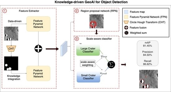
Although popular, directly applying the Faster R-CNN still cannot yield high-quality prediction due to the challenging nature of Mars crater detection. The following sections introduce three new features added to Faster R-CNN (Figure 3) to enable scale-aware, knowledge-driven deep learning for automated Mars crater detection.
3.3. Feature Pyramid Network (FPN)-Based Feature Extractor
The distribution of the crater BBOX size in Figure 2 shows that the scale range of the craters is very large. Therefore, ability to detect objects in a multi-scale context is important for the detection model. In the original Faster R-CNN -based detection pipeline, the model utilizes only the (late) feature map resulting from the last convolution layer. As discussed, a feature map created from the deeper network will contain high-level semantics of the image, that is, object relationships. Its dimension is much smaller than a feature map generated in the early convolutional layers. Correspondingly, small objects will be dissolved and often represented in less than one pixel in the late feature maps (refer to component 1 in Figure 3). Hence, using the late features alone will reduce the detection performance of small craters. To achieve multi-scale deep learning, we replace the feature extractor with a feature pyramid network (FPN) [59]. As shown in Figure 3, an FPN consists of an encoder-decoder structure. The encoder takes an image as input and hierarchically computes features layer by layer. The spatial dimension of feature maps is gradually reduced. It is easier to capture larger objects in later feature maps and smaller objects in earlier feature maps. Inherently, the encoder generates feature maps of different scales at different convolution stages. In comparison to the image pyramid approach, FPN reduces the computation time by efficiently constructing multi-scale features from a single resolution image.
However, the semantic information is not equally strong at each level. The high-resolution maps (early features) contain only low-level semantics, that is, texture and edges, and are therefore limited in their interpreting power. To enhance the weak semantics of early features, the decoder successively aggregates information from later layers into earlier layers and gradually recovers the object semantic details in a top-down manner with lateral connections. Iteratively, the later, coarser but semantically stronger feature map is upsampled to the same size as the feature map in the earlier layer. The earlier feature map also undergoes a convolutional operation to reduce the number of channels in order to fix the number of channels of the final feature map. Both feature maps are then merged to create rich semantics at all scales.
Finally, a convolution is applied on the merged feature map to generate the final feature map. This is to reduce the aliasing effect during the upsampling operation. Feature maps at all scales are then sent to the RPN and the classifier for crater detection.
3.4. Domain Knowledge Integration with the Data-Driven Model
Besides the multi-scale improvement of the feature extractor, we also explore how domain knowledge can be integrated into the data-driven learning framework to further empower the detection model. In traditional CDAs, the crater rim is often considered an important feature to localize a crater. Therefore, we explicitly incorporate the rim feature as prior knowledge into the model.
The first step is to trace and extract the crater rim in the images using CHT [41,75]. CHT is a feature extraction technique used in image processing for detecting circles. It is a commonly used strategy and has been applied in a number of CDAs [20,76]. The basic idea is to vote centroid candidates from each edge point using every possible radius and identify a circle using the highest voted centroid and radius. Figure 4 demonstrates the resultant images after CHT using the same images in Figure 1. The area in white indicates circles found in the images. In this study, the CHT is conducted during the preprocessing step which is not involved in the training phase so this extra process will not affect the model’s efficiency.
The second step is to integrate the identified rim feature into the detection network. As shown in Figure 3 (Component labeled as 2), this is achieved by adding another FPN as a feature extractor running in parallel with the original FPN. Each stage of the new FPN generates a feature map of the same dimension as the output of the FPN applied on the original input image. Two dimension-identical feature maps are then concatenated together. For the RPN or the classifier, the input becomes a feature map with twice the channels. Therefore, a convolution operation is applied to reduce the channel dimensions to the same number as before. Compared to the single FPN, the data propagation in the two FPN structures can be easily implemented in parallel so the overall execution time will increase only by 5%.
3.5. Scale-Aware Object Classification
For crater detection, the large size variance not only introduces the feature scale difference but also completely different features. For example, large craters appear with central peaks or multi-ring basins while small craters exhibit obscure bowl structures. This large intra-class feature variance may dramatically reduce detection performance because the original pipeline utilizes only a single classifier. Therefore, we replace the classifier by a scale-aware classifier [62]. The scale-aware classifier assembles two scale specific sub-networks for large and small craters, respectively, and uses a scale gate function to adaptively combine detection results of the sub-networks.
Figure 3 (Component labeled 3) shows the structure of the scale-aware classifier. The classifier takes the feature map at each level of the FPN and the crater proposals from the RPN as inputs. Two sub-networks generate category-level confidence scores and BBOX regressions like the original classifier in the Faster R-CNN. The detection results are then combined using a weighted sum with weights given by a scale-aware weighting layer. The scale-aware weights assigned to the two sub-networks make them specifically focus on their targeted crater sizes.
Intuitively, the weighting layer assigns a higher weight to the large-size sub-network when the crater has a large size. Otherwise, it gives a higher weight to the small-size sub-network. Suppose the weight for the large-size sub-network is , the weight for the small-size sub-network is and the input crater size is d, where d is defined as the length of a BBOX edge. Then, and are calculated as:
where is the average size of the craters in the training set and and are two learnable parameters. The ranges of and are from 0 to 1, and their sum is 1, a form of weighted sum to avoid the tendency of one model dominating the decision-making process over the other.
Once and are generated, the detection results from two sub-networks are simply combined using weighted sum. For example, the category-wise confidence scores of each proposal from large-size and small-size sub-networks are and , respectively. where is the score for the background and is the score for the crater from the sub-network x. The final score becomes
The final BBOX regressions are calculated using the same weighted sum approach. also has a range between 0 and 1, with 1 being high confidence and 0 being low confidence. The proposal receiving the highest score is chosen as the final prediction.
4. Experiments
4.1. Experiment Setup
We demonstrate the performance of the proposed model through a series of experiments using the generated crater images. The total number of images is 92,575 and the total number of craters is 192,036. We separate the images evenly into training and testing sets and both have the same geographical distribution on the Mars surface. This splitting strategy ensures that data in both sets have similar statistics. The training set includes 46,288 images (96,481 craters) and the testing set includes 46,287 images (95,555 craters).
We compare our method with the baseline model Faster R-CNN [72]. Faster R-CNN is the first phenomenal work that uses CNNs for feature extraction, region proposal, and classification in an end-to-end manner. It improves not only the detection performance but also computational efficiency. Based on Faster R-CNN, FPN introduces a feature pyramid to the backbone feature extractor to achieve multi-scale detections without sacrificing speed. It generates semantically rich feature maps at all levels via a top-down pathway and lateral connections. Five feature maps of different scales are sent to the RPN. The maximum number of proposals before reduction (NMS) at each level is 2000 so the total number of proposals is 10,000. To make a fair comparison, we increase the maximum number of proposals of Faster R-CNN to 10,000, also. Besides integrating FPN, our method includes two additional improvements: domain knowledge integration (D) and scale-aware classifier (S). We provide a detailed comparison of the performance contribution of each modification.
The evaluation metrics used in this work are precision, recall and mAP. Precision and recall are standard metrics in the CDA works which refer to the proportion of correct predictions and the proportion of ground truths that are identified, respectively. In the object detection task, a score is given to every detection. Therefore, a predefined detection threshold determines valid predictions and affects the precision and recall calculation. In this work, we use 0.5 as the detection threshold, and also demonstrate how this value affects the final result. mAP is a popular metric to evaluate deep learning-based object detection models. In comparison to precision and recall, mAP further measures how well the model finds all ground truths by ranking all the possible predictions. A model performs better if it finds more ground truths in the top-K predictions.
Ablation experiments are also conducted to investigate the impact of different parameters in the proposed method, for example, how does the number and size of the training images affect the detection results? The models were developed with the PyTorch [77] machine learning framework. ResNet50 (pretrained on ImageNet) is used as the feature extractor for both the Faster-RCNN and our proposed models. All models are trained with stochastic gradient descent (SGD) optimization algorithm. The hyperparameters include an initial learning rate 0.005 and a momentum value 0.9. Furthermore, a learning rate scheduler is used to decay the learning rate to 0.001 after 30 epochs. One epoch means having the entire dataset passed through the network once. Total number of epochs is set to 50. The experiments were conducted on Amazon’s EC2 platform using a g4dn.xlarge instance. The g4dn.xlarge instance on AWS provides 4 vCPUs, 16 GB memory and 1 NVIDIA T4 GPU with 16 GB memory. The 100 GB elastic block storage (EBS) was used to store the training and testing data as well as trained models.
Experiment 1 (Section 4.2) compare the performance of the baseline Faster R-CNN model with our proposed improvement. Experiment 2 (Section 4.3) further illustrates the impact of the detection threshold on the final results in terms of precision and recall. Experiment 3 (Section 4.4) investigates the influence of the proposed methods on the model’s efficiency. Section 4.5 presents the detection results.
4.2. Model Comparison
In Experiment 1, we compared the baseline model (Faster R-CNN) with our proposed improvements (FPN, domain knowledge integration (D) and scale-aware classifier (S)). The information presented in Table 1 demonstrates the detection results in terms of total number of predictions (with detection threshold set to be 0.5), precision, recall, and mAP. Overall, the proposed model combining the proposed strategies outperforms the baseline model for all evaluation metrics. In comparison, Faster R-CNN performs worse than other models without the adoption of multi-scale future maps. Compared to the network integrating FPN only (we call it FPN for short), the FPN + D model generates more predictions with a higher recall. This is because the CHT module guides the network to locate potential crater locations and increases the information intensity of the feature maps, thereby ensuring detection of more possible craters. However, the semantic ambiguity due to large variation of crater sizes complicates the detection process using a single classifier. This results in a lower precision than FPN. This issue is well addressed by the integration with a multi-scale classifier S. As Table 1 shows, the FPN + S model is capable of generating more accurate results (higher precision) by separating the decision process for large and small craters. Surprisingly, the FPN + S model also increases the recall rate with fewer predictions. By analyzing the results of FPN and FPN + S, we conclude that the scale-aware classifier not only eliminates the decision ambiguity between craters of different sizes but also helps the model to distinguish between craters and non-craters. The results of the two models (FPN + D and FPN + S) verify that our proposed methods work well from both the precision and recall perspectives. The final model (FPN + D + S) yields a significant increase (13% and 20.6% in precision and recall) than the Faster-RCNN model and yields a 10.37% and 4.75% increase in precision and recall, respectively, than FPN. It also achieves the state-of-the-art performance in the mAP metric. This result verifies the outstanding performance of the proposed model compared to existing solutions.
4.3. Detection Threshold
The outputs of object detection models come with scores. The score represents the confidence level associated with each prediction and is usually transferred into a softmax score within [0, 1]. We can specify a cutoff threshold after training to determine what is a “good” match. Predictions below the threshold will be removed and not considered further. In our proposed network, the threshold is probably the most important hyperparameter. It determines the number of objects that will be identified as craters. A high threshold will let a few crater candidates to pass the model, resulting probably in a high precision but a low recall. A low threshold value will instead result in more detections, but the results may not be as good in quality as those receiving a high probability score. In this scenario, recall rate may increase but precision may be lowered. Hence, an improper threshold value may lead to much extra work to filter out false positives or become unhelpful for crater cataloging. Therefore, we investigate how detection threshold impacts the predictive performance. In experiment 2, three different threshold values are chosen: 0, 0.3, and 0.5, and two models (raw FPN and our proposed model) are compared in terms of number of predictions, precision, and recall. The results are shown in Table 2. It is obvious that the number of predictions decreases as the threshold value increases. However, in comparison of the two models, our proposed model (FPN + D + S) has fewer predictions than FPN under the same threshold value. From the previous experiment, we found that this is mainly due to the integration of the scale-aware classifier which allows the discerning of crater from non-crater objects. By removing a large portion of false positive predictions, our proposed model yields both higher precision and recall than the FPN model. The results reflect a general trend that the higher the threshold that is utilized, the higher the precision it will achieve. At the same time, the recall will be lower. This experiment also allows us to identify the trade-offs between accuracy and efficiency and provides a general guideline for assigning a proper threshold value to each task to obtain a satisfactory result. For example, the recall can be as high as 92.01% if we choose the threshold value to be 0, but the model may spend lots of time removing incorrect predictions (about 30% of the total predictions). Although it locates most of the potential craters, this value is chosen only when cataloging all craters in a given area is the most important requirement.
4.4. Computational Efficiency
In this experiment, we compare the unit training and inference (prediction) time among different models. The training time is measured as the time cost per iteration, which includes calculating the prediction and loss (forward propagation) and updating the model parameter (backward propagation) of the network. The inference time is measured as the time cost of the forward propagation for a single image. Both runtimes are measured on NVIDIA T4 GPUs. Several points are noteworthy given the results in Table 3. First, although the structure of Faster R-CNN is simpler than FPN, its training and inference time are more than FPN. The reason lies in the time-consuming operation for NMS, which is used to remove overlapping proposals and has runtime where n is the number of proposals. In order to have a fair comparison, we make the total number of proposals the same between Faster R-CNN and FPN. However, FPN generates proposals from five different feature maps and Faster R-CNN uses only the feature map from the last convolution layer. This results in Faster R-CNN running NMS with a large number of proposals (10,000) while FPN runs NMS separately with a small number of proposals (2000) at each level. Therefore, Faster R-CNN spends more time on the training and inference even though FPN contains more convolution operations. Because FPN performs better than Faster R-CNN, we further compare the efficiency of our proposed strategies over the FPN.
Second, FPN + D (Domain Knowledge Integration) model is about 1.6x–1.7x slower than FPN on a single-GPU implementation. This is due to an additional backbone feature extractor, and the operations execute in a sequential order in two backbone feature extractors. To further improve efficiency, model parallelism can be utilized because one of the two backbones is sitting idle throughout the execution and the operations in two backbones are independent. We split two backbones onto two GPUs and the computed feature maps are combined in one of the GPUs. The result shows that the time cost of the model’s parallel implementation is only about 5% longer than the FPN. This is due to the overhead in copying data back and forth across the GPUs. Besides, the time consumption of the FPN + D model does not include the rim feature calculation for domain knowledge integration. Such operations can be computed in the pre-processing step and will not influence training and inference efficiency. Next, the additional sub-network (classifier) of FPN + S model introduces the extra time cost compared to the FPN. The 15% slower speed yields an 8.5% increase in precision, 2.21% increase in recall, and 1.63% increase in mAP. Finally, the combination of D and S modules (FPN + D + S) increases the time by almost twice that of the FPN in the single-GPU implementation. Like the FPN + D network, we can apply model parallelism to reduce the time cost. This results in 25%–30% more time than the FPN with over 3%–10% improvement in all evaluation metrics.
4.5. Detection Results
Figure 5 demonstrates the crater prediction results (in blue box) and the ground-truth labels (in red box) of our proposed model. The figures show that the model performs well in detecting all labeled craters. Figure 5a,b demonstrate that craters can be detected even though the size variance is large. The model is also capable of predicting multiple craters of the same size (Figure 5c) or different sizes (Figure 5d) in the same image scene. Interestingly, the BBOX predicted by the model is also of higher quality than the ground-truth labels. In addition, the model can not only detect labeled craters, but it can also capture craters which are not yet included in the Robbin’s database (Figure 5e,f). Through visual inspection, they are likely to be craters. Besides these new predictions, there are also crater-like features that are not detected by the model (Figure 5f).
To further evaluate the model performance (model with FPN + D + S), the cumulative plots were generated for analyzing the model’s predictive performance against the 46,287 testing images. The number of ground truth labels, the model detection results, true positive, false positive and false negative results at different crater sizes are presented. Among which, true positive results are correct detections from the model; false positive results refer to the non-crater objects detected as craters; false negative results refer to craters failed to be detected by the model. Figure 6a shows the accumulative plot for all the results and Figure 6b shows part of the results with crater size smaller than 50 pixels (5 km in diameter). The results show that (1) the model predicted more results (orange line) than the ground-truth data (blue line), but the difference is small; (2) the number of true positive results are about three times as many as the false positive results; and (3) most false positive results are detected in smaller craters (with diameter smaller than 5 km/50 pixels). A portion of these false negatives might be craters (blue-only boxes in Figure 5). They will be further analyzed through joint efforts with Earth and space scientists. If our assumption is true, our model actually has higher prediction accuracy than the current numbers. These findings can be used to further enrich the knowledge about Mars’ craters and the land surface processes on Mars.
Overall, the proposed GeoAI model has demonstrated its outstanding capability in the automated detection of Mars craters. Besides advanced models, we have carefully prepared the training and testing datasets that have both global coverage and geographical representativeness of Mars craters. Different from existing solutions, especially the CDA algorithms applied to a specific region, our model is capable of handling and extracting prominent image features from Mars craters distributed at a global scale. This way, model generalization and scalability can both be achieved. Our GeoAI model can serve as an effective tool for enriching existing Mars crater databases and correcting the location information of the logged craters.
5. Conclusions and Future Work
We have presented a GeoAI framework for building an accurate crater detection system. By injecting the domain knowledge and enabling the scale-aware learning, our method shows obvious improvements over existing object detection models with deep learning. Furthermore, the system presents a methodology for significantly reducing the time for cataloging new craters. What enables such a conversion is the convergence research between computer scientists, and Earth and space scientists. Computer science researchers provide expertise in image processing. Models for general object detection and localization have been extensively developed in the community. Utilizing the domain knowledge of crater data and features from geospatial scientists enables domain-specific improvement to the proposed model. The integration of data-driven and knowledge-driven analytics yield important results in automated crater cataloging.
In the future, we will further improve two aspects of our research program: data and methodology. From the training data perspective, many craters were removed during training data generation which results in incomplete crater cataloging in the benchmark dataset. An enhanced data split and merge strategy will be developed to leverage the model’s capabilities to the entire Mars craters. Next, although Robbins’ crater database contains over 380,000 impact craters on Mars, a large number of small craters with diameters less than 1 km have not been included in the database. From the methodology perspective, while we have successfully shown the accurate detection results of our model, efficiency optimization becomes the next stage of work. One possible strategy is to combine the RPN and the object classifier such that the detection framework can be transformed to the more efficient, single stage learning. We will also integrate multi-source data, such as remote sensing images and the Mars elevation dataset, into the deep learning model to further improve the detection accuracy. The model and data in this work will be open sourced to encourage more researchers to jointly tackle this exciting research area.
Author Contributions
Conceptualization, W.L.; methodology, C.-Y.H. and W.L.; software, C.-Y.H. and S.W.; validation, C.-Y.H. and W.L.; formal analysis, C.-Y.H.; investigation, W.L.; resources, W.L.; data curation, C.H and S.W.; writing—original draft preparation, C.-Y.H., W.L. and S.W.; writing—review and editing, W.L.; visualization, C.-Y.H. and W.L.; supervision, W.L.; project administration, W.L.; funding acquisition, W.L. All authors have read and agreed to the published version of the manuscript.
Funding
This work is in part supported by the National Science Foundation under grants BCS-1853864, BCS-1455349, OIA-2033521, OIA-1936677, and OIA-1937908.
Institutional Review Board Statement
Not applicable.
Informed Consent Statement
Not applicable.
Conflicts of Interest
The authors declare no conflict of interest.
Abbreviations
The following abbreviations are used in this manuscript:
| GeoAI | Geospatial Artificial Intelligence |
| DEM | digital elevation model |
| CDA | Crater detection algorithm |
| CNN | Convolutional neural network |
| mAP | Mean Average Precision |
| BBOX | Bounding box |
| THEMIS | Thermal Emission Imagining System |
| DIR | Daytime infrared |
| RPN | Region proposal network |
| NMS | Non-maximum suppression |
| RoI | Region of interest |
| FPN | Feature pyramid network |
| CHT | Circular Hough Transform |
References
- Barlow, N.G. A review of Martian impact crater ejecta structures and their implications for target properties. Large Meteor. Impacts III 2005, 384, 433–442. [Google Scholar]
- Barlow, N.G.; Perez, C.B. Martian impact crater ejecta morphologies as indicators of the distribution of subsurface volatiles. J. Geophys. Res. Planets 2003, 108. [Google Scholar] [CrossRef] [Green Version]
- Hartmann, W.K.; Malin, M.; McEwen, A.; Carr, M.; Soderblom, L.; Thomas, P.; Danielson, E.; James, P.; Veverka, J. Evidence for recent volcanism on Mars from crater counts. Nature 1999, 397, 586–589. [Google Scholar] [CrossRef]
- Hawke, B.; Head, J. Impact melt on lunar crater rims. In Impact and Explosion Cratering: Planetary and Terrestrial Implications; Pergamon Press: New York, NY, USA, 1977; pp. 815–841. [Google Scholar]
- Neukum, G.; Wise, D. Mars—A standard crater curve and possible new time scale. Science 1976, 194, 1381–1387. [Google Scholar] [CrossRef] [PubMed]
- Hartmann, W.K. Martian cratering. Icarus 1966, 5, 565–576. [Google Scholar] [CrossRef]
- Schon, S.C.; Head, J.W.; Fassett, C.I. Recent high-latitude resurfacing by a climate-related latitude-dependent mantle: Constraining age of emplacement from counts of small craters. Planet. Space Sci. 2012, 69, 49–61. [Google Scholar] [CrossRef]
- Schaber, G.; Strom, R.; Moore, H.; Soderblom, L.A.; Kirk, R.L.; Chadwick, D.; Dawson, D.; Gaddis, L.; Boyce, J.; Russell, J. Geology and distribution of impact craters on Venus: What are they telling us? J. Geophys. Res. Planets 1992, 97, 13257–13301. [Google Scholar] [CrossRef]
- Wilhelms, D.E.; John, F.; Trask, N.J. The Geologic History of the Moon; Technical Report; U.S. Geological Survey, 1987. Available online: https://pubs.er.usgs.gov/publication/pp1348 (accessed on 27 May 2021).
- Martín-Torres, F.J.; Zorzano, M.P.; Valentín-Serrano, P.; Harri, A.M.; Genzer, M.; Kemppinen, O.; Rivera-Valentin, E.G.; Jun, I.; Wray, J.; Madsen, M.B.; et al. Transient liquid water and water activity at Gale crater on Mars. Nat. Geosci. 2015, 8, 357–361. [Google Scholar] [CrossRef]
- Ruff, S.W.; Farmer, J.D. Silica deposits on Mars with features resembling hot spring biosignatures at El Tatio in Chile. Nat. Commun. 2016, 7, 1–10. [Google Scholar] [CrossRef] [PubMed]
- Losiak, A.; Wilhelms, D.; Byrne, C.; Thaisen, K.; Weider, S.; Kohout, T.; O’Sullivan, K.; Kring, D. A new lunar impact crater database. In Lunar and Planetary Science Conference; 2009; p. 1532. Available online: https://www.lpi.usra.edu/meetings/lpsc2009/pdf/1532.pdf (accessed on 27 May 2021).
- Robbins, S.J. A global lunar crater database, complete for craters 1 km, ii. In Proceedings of the 48th Lunar and Planetary Science Conference, The Woodlands, TX, USA, 20–24 March 2017; pp. 20–24. [Google Scholar]
- Robbins, S.J.; Hynek, B.M. A new global database of Mars impact craters ≥1 km: 1. Database creation, properties, and parameters. J. Geophys. Res. Planets 2012, 117. [Google Scholar] [CrossRef]
- Schaber, G.G.; Chadwick, D.J. Venus’ impact-crater database: Update to approximately 98 percent of the planet’s surface. In Proceedings of the Lunar and Planetary Science Conference XXIV, Houston, TX, USA, 15–19 March 1993; Volume 24, p. 1241. [Google Scholar]
- Edwards, C.; Nowicki, K.; Christensen, P.; Hill, J.; Gorelick, N.; Murray, K. Mosaicking of global planetary image datasets: 1. Techniques and data processing for Thermal Emission Imaging System (THEMIS) multi-spectral data. J. Geophys. Res. Planets 2011, 116. [Google Scholar] [CrossRef]
- Di, K.; Li, W.; Yue, Z.; Sun, Y.; Liu, Y. A machine learning approach to crater detection from topographic data. Adv. Space Res. 2014, 54, 2419–2429. [Google Scholar] [CrossRef]
- Honda, R.; Konishi, O.; Azuma, R.; Yokogawa, H.; Yamanaka, S.; Iijima, Y. Data mining system for planetary images-crater detection and categorization. In Proceedings of the International Workshop on Machine Learning of Spatial Knowledge in Conjunction with ICML, Stanford, CA, USA, 2000; pp. 103–108. Available online: http://citeseerx.ist.psu.edu/viewdoc/versions?doi=10.1.1.28.1172 (accessed on 27 May 2021).
- Jahn, H. Crater detection by linear filters representing the Hough Transform. In Proceedings of the ISPRS Commission III Symposium: Spatial Information from Digital Photogrammetry and Computer Vision, Munich, Germany, 5–9 September 1994; International Society for Optics and Photonics: Bellingham, WA, USA, 1994; Volume 2357, pp. 427–431. [Google Scholar]
- Kim, J.R.; Muller, J.P.; van Gasselt, S.; Morley, J.G.; Neukum, G. Automated crater detection, a new tool for Mars cartography and chronology. Photogramm. Eng. Remote Sens. 2005, 71, 1205–1217. [Google Scholar] [CrossRef] [Green Version]
- Lee, C. Automated crater detection on Mars using deep learning. Planet. Space Sci. 2019, 170, 16–28. [Google Scholar] [CrossRef] [Green Version]
- Palafox, L.F.; Hamilton, C.W.; Scheidt, S.P.; Alvarez, A.M. Automated detection of geological landforms on Mars using Convolutional Neural Networks. Comput. Geosci. 2017, 101, 48–56. [Google Scholar] [CrossRef]
- Wetzler, P.G.; Honda, R.; Enke, B.; Merline, W.J.; Chapman, C.R.; Burl, M.C. Learning to detect small impact craters. In Proceedings of the 2005 Seventh IEEE Workshops on Applications of Computer Vision (WACV/MOTION’05)-Volume 1, Breckenridge, CO, USA, 5–7 January 2005; Volume 1, pp. 178–184. [Google Scholar]
- Li, W. GeoAI: Where machine learning and big data converge in GIScience. J. Spat. Inf. Sci. 2020, 2020, 71–77. [Google Scholar] [CrossRef]
- Li, W.; Hsu, C.Y. Automated terrain feature identification from remote sensing imagery: A deep learning approach. Int. J. Geogr. Inf. Sci. 2020, 34, 637–660. [Google Scholar] [CrossRef]
- Li, W.; Hsu, C.Y.; Hu, M. Tobler’s First Law in GeoAI: A spatially explicit deep learning model for terrain feature detection under weak supervision. Ann. Am. Assoc. Geogr. 2021. [Google Scholar] [CrossRef]
- DeLatte, D.; Crites, S.T.; Guttenberg, N.; Yairi, T. Automated crater detection algorithms from a machine learning perspective in the convolutional neural network era. Adv. Space Res. 2019, 64, 1615–1628. [Google Scholar] [CrossRef]
- Tewari, A.; Verma, V.; Srivastava, P.; Jain, V.; Khanna, N. Automated Crater Detection from Co-registered Optical Images, Elevation Maps and Slope Maps using Deep Learning. arXiv 2020, arXiv:2012.15281. [Google Scholar]
- Li, H.; Jiang, B.; Li, Y.; Cao, L. A combined method of crater detection and recognition based on deep learning. Syst. Sci. Control Eng. 2020, 9, 132–140. [Google Scholar] [CrossRef]
- Lee, C.; Hogan, J. Automated crater detection with human level performance. Comput. Geosci. 2021, 147, 104645. [Google Scholar] [CrossRef]
- Wang, H.; Jiang, J.; Zhang, G. CraterIDNet: An end-to-end fully convolutional neural network for crater detection and identification in remotely sensed planetary images. Remote Sens. 2018, 10, 1067. [Google Scholar] [CrossRef] [Green Version]
- Hsu, C.Y.; Li, W. Learning from counting: Leveraging temporal classification for weakly supervised object localization and detection. arXiv 2021, arXiv:2103.04009. [Google Scholar]
- Ghorbanzadeh, O.; Tiede, D.; Wendt, L.; Sudmanns, M.; Lang, S. Transferable instance segmentation of dwellings in a refugee camp-integrating CNN and OBIA. Eur. J. Remote Sens. 2021, 54, 127–140. [Google Scholar] [CrossRef]
- Li, Y.; Ouyang, S.; Zhang, Y. Collaboratively boosting data-driven deep learning and knowledge-guided ontological reasoning for semantic segmentation of remote sensing imagery. arXiv 2020, arXiv:2010.02451. [Google Scholar]
- Cheng, G.; Xie, X.; Han, J.; Guo, L.; Xia, G.S. Remote sensing image scene classification meets deep learning: Challenges, methods, benchmarks, and opportunities. IEEE J. Sel. Top. Appl. Earth Obs. Remote Sens. 2020, 13, 3735–3756. [Google Scholar] [CrossRef]
- Yu, M.; Cui, H.; Tian, Y. A new approach based on crater detection and matching for visual navigation in planetary landing. Adv. Space Res. 2014, 53, 1810–1821. [Google Scholar] [CrossRef]
- Arvidson, R.E. Morphologic classification of Martian craters and some implications. Icarus 1974, 22, 264–271. [Google Scholar] [CrossRef]
- Cintala, M.J.; Head, J.W.; Mutch, T.A. Martian crater depth/diameter relationships-Comparison with the moon and Mercury. Lunar Planet. Sci. Conf. Proc. 1976, 7, 3575–3587. [Google Scholar]
- Emami, E.; Bebis, G.; Nefian, A.; Fong, T. Automatic crater detection using convex grouping and convolutional neural networks. In International Symposium on Visual Computing; Springer: Berlin, Germany, 2015; pp. 213–224. [Google Scholar]
- Stepinski, T.F.; Mendenhall, M.P.; Bue, B.D. Machine cataloging of impact craters on Mars. Icarus 2009, 203, 77–87. [Google Scholar] [CrossRef]
- Hough, P.V. Method and Means for Recognizing Complex Patterns. U.S. Patent 3,069,654, 18 December 1962. [Google Scholar]
- Silburt, A.; Ali-Dib, M.; Zhu, C.; Jackson, A.; Valencia, D.; Kissin, Y.; Tamayo, D.; Menou, K. Lunar crater identification via deep learning. Icarus 2019, 317, 27–38. [Google Scholar] [CrossRef] [Green Version]
- Yoo, J.C.; Han, T.H. Fast normalized cross-correlation. Circuits Syst. Signal Process. 2009, 28, 819–843. [Google Scholar] [CrossRef]
- Emami, E.; Ahmad, T.; Bebis, G.; Nefian, A.; Fong, T. Crater detection using unsupervised algorithms and convolutional neural networks. IEEE Trans. Geosci. Remote Sens. 2019, 57, 5373–5383. [Google Scholar] [CrossRef]
- Ronneberger, O.; Fischer, P.; Brox, T. U-net: Convolutional networks for biomedical image segmentation. In International Conference on Medical Image Computing and Computer-Assisted Intervention; Springer: Berlin, Germany, 2015; pp. 234–241. [Google Scholar]
- Yang, J.; Kang, Z. Bayesian network-based extraction of lunar impact craters from optical images and DEM data. Adv. Space Res. 2019, 63, 3721–3737. [Google Scholar] [CrossRef]
- Zuo, W.; Li, C.; Yu, L.; Zhang, Z.; Wang, R.; Zeng, X.; Liu, Y.; Xiong, Y. Shadow–highlight feature matching automatic small crater recognition using high-resolution digital orthophoto map from Chang’E Missions. Acta Geochim. 2019, 38, 541–554. [Google Scholar] [CrossRef]
- He, K.; Gkioxari, G.; Dollár, P.; Girshick, R. Mask r-cnn. In Proceedings of the IEEE International Conference on Computer Vision, Venice, Italy, 22–29 October 2017; pp. 2961–2969. [Google Scholar]
- Barata, T.; Alves, E.I.; Saraiva, J.; Pina, P. Automatic recognition of impact craters on the surface of Mars. In International Conference Image Analysis and Recognition; Springer: Berlin, Germany, 2004; pp. 489–496. [Google Scholar]
- Plesko, C.; Brumby, S.; Asphaug, E. A Comparison of Automated and Manual Surveys of Small Craters in Elysium Planitia. In Proceedings of the 36th Annual Lunar and Planetary Science Conference, The Woodlands, TX, USA, 16–20 March 2005; p. 1971. [Google Scholar]
- Barlow, N.G. Crater size-frequency distributions and a revised Martian relative chronology. Icarus 1988, 75, 285–305. [Google Scholar] [CrossRef]
- Dalal, N.; Triggs, B. Histograms of oriented gradients for human detection. In Proceedings of the 2005 IEEE Computer Society Conference on Computer Vision and Pattern Recognition (CVPR’05), San Diego, CA, USA, 20–25 June 2005; Volume 1, pp. 886–893. [Google Scholar]
- He, K.; Zhang, X.; Ren, S.; Sun, J. Spatial pyramid pooling in deep convolutional networks for visual recognition. IEEE Trans. Pattern Anal. Mach. Intell. 2015, 37, 1904–1916. [Google Scholar] [CrossRef] [Green Version]
- Shrivastava, A.; Gupta, A.; Girshick, R. Training region-based object detectors with online hard example mining. In Proceedings of the IEEE Conference on Computer Vision and Pattern Recognition, Las Vegas, NV, USA, 27–30 June 2016; pp. 761–769. [Google Scholar]
- Hariharan, B.; Arbeláez, P.; Girshick, R.; Malik, J. Hypercolumns for object segmentation and fine-grained localization. In Proceedings of the IEEE Conference on Computer Vision and Pattern Recognition, Boston, MA, USA, 7–12 June 2015; pp. 447–456. [Google Scholar]
- Kong, T.; Yao, A.; Chen, Y.; Sun, F. Hypernet: Towards accurate region proposal generation and joint object detection. In Proceedings of the IEEE Conference on Computer Vision and Pattern Recognition, Las Vegas, NV, USA, 27–30 June 2016; pp. 845–853. [Google Scholar]
- Liu, W.; Anguelov, D.; Erhan, D.; Szegedy, C.; Reed, S.; Fu, C.Y.; Berg, A.C. Ssd: Single shot multibox detector. In European Conference on Computer Vision; Springer: Berlin, Germany, 2016; pp. 21–37. [Google Scholar]
- Honari, S.; Yosinski, J.; Vincent, P.; Pal, C. Recombinator networks: Learning coarse-to-fine feature aggregation. In Proceedings of the IEEE Conference on Computer Vision and Pattern Recognition, Las Vegas, NV, USA, 27–30 June 2016; pp. 5743–5752. [Google Scholar]
- Lin, T.Y.; Dollár, P.; Girshick, R.; He, K.; Hariharan, B.; Belongie, S. Feature pyramid networks for object detection. In Proceedings of the IEEE Conference on Computer Vision and Pattern Recognition, Honolulu, HI, USA, 21–26 July 2017; pp. 2117–2125. [Google Scholar]
- Pinheiro, P.O.; Lin, T.Y.; Collobert, R.; Dollár, P. Learning to refine object segments. In European Conference on Computer Vision; Springer: Berlin, Germany, 2016; pp. 75–91. [Google Scholar]
- Cai, Z.; Fan, Q.; Feris, R.S.; Vasconcelos, N. A unified multi-scale deep convolutional neural network for fast object detection. In European Conference on Computer Vision; Springer: Berlin, Germany, 2016; pp. 354–370. [Google Scholar]
- Li, J.; Liang, X.; Shen, S.; Xu, T.; Feng, J.; Yan, S. Scale-aware fast R-CNN for pedestrian detection. IEEE Trans. Multimed. 2017, 20, 985–996. [Google Scholar] [CrossRef] [Green Version]
- Xu, Y.; Xiao, T.; Zhang, J.; Yang, K.; Zhang, Z. Scale-invariant convolutional neural networks. arXiv 2014, arXiv:1411.6369. [Google Scholar]
- Tan, M.; Pang, R.; Le, Q.V. Efficientdet: Scalable and efficient object detection. In Proceedings of the IEEE/CVF Conference on Computer Vision and Pattern Recognition, Seattle, WA, USA, 14–19 June 2020; pp. 10781–10790. [Google Scholar]
- Everingham, M.; Van Gool, L.; Williams, C.K.; Winn, J.; Zisserman, A. The pascal visual object classes (voc) challenge. Int. J. Comput. Vis. 2010, 88, 303–338. [Google Scholar] [CrossRef] [Green Version]
- Lin, T.Y.; Maire, M.; Belongie, S.; Hays, J.; Perona, P.; Ramanan, D.; Dollár, P.; Zitnick, C.L. Microsoft coco: Common objects in context. In European Conference on Computer Vision; Springer: Berlin, Germany, 2014; pp. 740–755. [Google Scholar]
- Dollár, P.; Wojek, C.; Schiele, B.; Perona, P. Pedestrian detection: A benchmark. In Proceedings of the 2009 IEEE Conference on Computer Vision and Pattern Recognition, Miami Beach, FL, USA, 20–25 June 2009; pp. 304–311. [Google Scholar]
- Bandeira, L.; Ding, W.; Stepinski, T. Automatic detection of sub-km craters using shape and texture information. In Proceedings of the Lunar and Planetary Science Conference, The Woodlands, TX, USA, 1–5 March 2010; p. 1144. [Google Scholar]
- McEwen, A.S.; Eliason, E.M.; Bergstrom, J.W.; Bridges, N.T.; Hansen, C.J.; Delamere, W.A.; Grant, J.A.; Gulick, V.C.; Herkenhoff, K.E.; Keszthelyi, L.; et al. Mars reconnaissance orbiter’s high resolution imaging science experiment (HiRISE). J. Geophys. Res. Planets 2007, 112. [Google Scholar] [CrossRef] [Green Version]
- Smith, D.E.; Zuber, M.T.; Frey, H.V.; Garvin, J.B.; Head, J.W.; Muhleman, D.O.; Pettengill, G.H.; Phillips, R.J.; Solomon, S.C.; Zwally, H.J.; et al. Mars Orbiter Laser Altimeter: Experiment summary after the first year of global mapping of Mars. J. Geophys. Res. Planets 2001, 106, 23689–23722. [Google Scholar] [CrossRef]
- Zuber, M.T.; Smith, D.; Solomon, S.; Muhleman, D.; Head, J.; Garvin, J.; Abshire, J.; Bufton, J. The Mars Observer laser altimeter investigation. J. Geophys. Res. Planets 1992, 97, 7781–7797. [Google Scholar] [CrossRef]
- Ren, S.; He, K.; Girshick, R.; Sun, J. Faster R-CNN: Towards real-time object detection with region proposal networks. IEEE Trans. Pattern Anal. Mach. Intell. 2016, 39, 1137–1149. [Google Scholar] [CrossRef] [Green Version]
- He, K.; Zhang, X.; Ren, S.; Sun, J. Deep residual learning for image recognition. In Proceedings of the IEEE Conference on Computer Vision and Pattern Recognition, Las Vegas, NV, USA, 27–30 June 2016; pp. 770–778. [Google Scholar]
- Long, J.; Shelhamer, E.; Darrell, T. Fully convolutional networks for semantic segmentation. In Proceedings of the IEEE Conference on Computer Vision and Pattern Recognition, Boston, MA, USA, 7–12 June 2015; pp. 3431–3440. [Google Scholar]
- Ballard, D.H. Generalizing the Hough transform to detect arbitrary shapes. Pattern Recognit. 1981, 13, 111–122. [Google Scholar] [CrossRef] [Green Version]
- Galloway, M.J.; Benedix, G.K.; Bland, P.A.; Paxman, J.; Towner, M.C.; Tan, T. Automated crater detection and counting using the Hough transform. In Proceedings of the 2014 IEEE International Conference on Image Processing (ICIP), Paris, France, 27–30 October 2014; pp. 1579–1583. [Google Scholar]
- Paszke, A.; Gross, S.; Massa, F.; Lerer, A.; Bradbury, J.; Chanan, G.; Killeen, T.; Lin, Z.; Gimelshein, N.; Antiga, L.; et al. Pytorch: An imperative style, high-performance deep learning library. arXiv 2019, arXiv:1912.01703. [Google Scholar]
Figure 1.
Examples of the training images and labels: (a) Single crater; (b) Multiple craters.

Figure 2.
Statistics from the generated Mars crater dataset. Each pixel edge is 100 m. (a) The cumulative image frequency plot in terms of number of craters within each image; (b) The cumulative crater frequency plot in terms of crater sizes. One pixel represents an 100 m × 100 m area; (c) The heat map distribution of all the craters in our training database.

Figure 3.
A knowledge-driven, scale-aware Mars crater detection pipeline. Components 1–3 in dashed boxes are new features of the model.
Figure 3.
A knowledge-driven, scale-aware Mars crater detection pipeline. Components 1–3 in dashed boxes are new features of the model.

Figure 4.
Results from Circular Hough Transform (CHT) on images shown in Figure 1: (a) Single crater; (b) Multiple craters.
Figure 4.
Results from Circular Hough Transform (CHT) on images shown in Figure 1: (a) Single crater; (b) Multiple craters.

Figure 5.
(a–f) illustrate sample detection results for Mars craters at different locations on the Mars surface. The ground-truth Bounding Boxes (BBOX) are labeled in red and model prediction results are the blue boxes.
Figure 5.
(a–f) illustrate sample detection results for Mars craters at different locations on the Mars surface. The ground-truth Bounding Boxes (BBOX) are labeled in red and model prediction results are the blue boxes.

Figure 6.
A detailed analysis of detection results: (a) Cumulative plot for ground-truth and model prediction results of craters of all sizes; (b) A closer look at the cumulative plot in (a) for ground-truth and model prediction results of craters with diameters less than 50 pixels (5 km).
Figure 6.
A detailed analysis of detection results: (a) Cumulative plot for ground-truth and model prediction results of craters of all sizes; (b) A closer look at the cumulative plot in (a) for ground-truth and model prediction results of craters with diameters less than 50 pixels (5 km).


Table 1.
Model comparison (threshold = 0.5). D: domain knowledge integration. S: scale-aware classifier.
Table 1.
Model comparison (threshold = 0.5). D: domain knowledge integration. S: scale-aware classifier.
| Models | Predictions | Precision (%) | Recall (%) | mAP (%) |
|---|---|---|---|---|
| Faster R-CNN [72] | 88,125 | 71.53 | 65.97 | 72.18 |
| FPN [59] | 105,539 | 74.13 | 81.87 | 78.09 |
| FPN + D | 115,121 | 69.70 | 83.97 | 76.16 |
| FPN + S | 97,231 | 82.63 | 84.08 | 79.72 |
| FPN + D + S | 97,956 | 84.50 | 86.62 | 81.45 |
Table 2.
Detection threshold comparison.
| Models | Threshold | Predictions | Precision (%) | Recall (%) | mAP (%) |
|---|---|---|---|---|---|
| FPN [59] | 0 | 140,864 | 55.92 | 85.97 | 78.09 |
| 0.3 | 109,001 | 69.96 | 83.22 | ||
| 0.5 | 105,539 | 74.13 | 81.87 | ||
| FPN + D + S | 0 | 128,524 | 68.40 | 92.01 | 81.45 |
| 0.3 | 103,907 | 81.09 | 88.18 | ||
| 0.5 | 97,956 | 84.50 | 86.62 |
Publisher’s Note: MDPI stays neutral with regard to jurisdictional claims in published maps and institutional affiliations. |
© 2021 by the authors. Licensee MDPI, Basel, Switzerland. This article is an open access article distributed under the terms and conditions of the Creative Commons Attribution (CC BY) license (https://creativecommons.org/licenses/by/4.0/).
Share and Cite
MDPI and ACS Style
Hsu, C.-Y.; Li, W.; Wang, S. Knowledge-Driven GeoAI: Integrating Spatial Knowledge into Multi-Scale Deep Learning for Mars Crater Detection. Remote Sens. 2021, 13, 2116. https://doi.org/10.3390/rs13112116
AMA Style
Hsu C-Y, Li W, Wang S. Knowledge-Driven GeoAI: Integrating Spatial Knowledge into Multi-Scale Deep Learning for Mars Crater Detection. Remote Sensing. 2021; 13(11):2116. https://doi.org/10.3390/rs13112116
Chicago/Turabian StyleHsu, Chia-Yu, Wenwen Li, and Sizhe Wang. 2021. "Knowledge-Driven GeoAI: Integrating Spatial Knowledge into Multi-Scale Deep Learning for Mars Crater Detection" Remote Sensing 13, no. 11: 2116. https://doi.org/10.3390/rs13112116
Note that from the first issue of 2016, this journal uses article numbers instead of page numbers. See further details here.