
Memory-Augmented Transformer for Remote Sensing Image Semantic Segmentation

1
Aerospace Information Research Institute, Chinese Academy of Sciences, Beijing 100190, China
2
Key Laboratory of Technology in Geo-Spatial Information Processing and Application System, Beijing 100190, China
3
School of Electronic, Electrical and Communication Engineering, University of Chinese Academy of Sciences, Beijing 101408, China
*
Author to whom correspondence should be addressed.
Remote Sens. 2021, 13(22), 4518; https://doi.org/10.3390/rs13224518
Submission received: 9 October 2021
/
Revised: 7 November 2021
/
Accepted: 8 November 2021
/
Published: 10 November 2021
(This article belongs to the Special Issue 2nd Edition GeoAI: Integration of Artificial Intelligence, Machine Learning and Deep Learning with Remote Sensing)
Abstract
:The semantic segmentation of remote sensing images requires distinguishing local regions of different classes and exploiting a uniform global representation of the same-class instances. Such requirements make it necessary for the segmentation methods to extract discriminative local features between different classes and to explore representative features for all instances of a given class. While common deep convolutional neural networks (DCNNs) can effectively focus on local features, they are limited by their receptive field to obtain consistent global information. In this paper, we propose a memory-augmented transformer (MAT) to effectively model both the local and global information. The feature extraction pipeline of the MAT is split into a memory-based global relationship guidance module and a local feature extraction module. The local feature extraction module mainly consists of a transformer, which is used to extract features from the input images. The global relationship guidance module maintains a memory bank for the consistent encoding of the global information. Global guidance is performed by memory interaction. Bidirectional information flow between the global and local branches is conducted by a memory-query module, as well as a memory-update module, respectively. Experiment results on the ISPRS Potsdam and ISPRS Vaihingen datasets demonstrated that our method can perform competitively with state-of-the-art methods.
1. Introduction
Semantic segmentation of high-resolution remote sensing images [1,2,3,4] is an important application scenario in remote sensing image interpretation, which is widely used in land mapping, environmental monitoring, urban construction, etc. Traditional methods [5,6] mainly depend on low-level features such as color, edge, shape, and spatial locations and use heuristic methods such as clustering or thresholding to translate the features into the final segmentation masks. Due to the limited representation power of low-level features and the overtuned parameters of the clustering methods, the performance of these methods is far from satisfactory. The emergence of deep convolutional neural networks (DCNNs) has equipped us with more powerful representation abilities and has boosted the performance of remote sensing image recognition. DCNNs [7,8] take the remote sensing image as the input and directly map the input image into the desired output (class, object boxes, and masks). In the remote sensing image semantic segmentation field, many works [9,10] using convolutional neural networks have been proposed to tackle the problem. The segmentation results are better than traditional methods thanks to the deep layers and the end-to-end training paradigm.
Most of the segmentation methods follow an encoder–decoder model design, as shown in Figure 1a. The encoder is used to encode the input image into latent representations, which may be a single-scale or multiscale representation. The decoder takes the latent representations as the input and decodes the representations into the final segmentation masks.
The encoder and decoder are stacked deep convolutional neural networks (DCNN) in most cases due to their favorable properties such as weight sharing and translation invariance. However, in high-resolution remote sensing images, instances often occupy more than a hundred pixels. In this case, to construct different class’s overall representations, the network must have a large receptive field. The local receptive field of convolution makes DCNNs hard to extend to such large areas and model long-range information. To enhance the long-range information modeling ability of DCNNs, many additional modules have been proposed, such as dilate convolution [11,12], the attention mechanism [13,14], and deformable convolution [15,16]. In this paper, rather than exploiting these modules to aggregate global information, we used a transformer [17] to directly model long-range connections. Unlike DCNNs, the transformer rearranges the spatial dimension of an image into a single dimension, and the rearranged feature unit is called a token or a patch. Self-attention is proposed in the transformer to calculate the similarity between every two tokens so every token can attend to all tokens. In this way, the transformer captures long-range information throughout the segmentation pipeline.
Though the transformer can construct long-range information effectively, the quadratic computational complexity with respect to the token number is unbearable even for modern GPUs. Moreover, The overemphasis on global information often leads to the degradation of the local information extraction ability. To alleviate such problems, the attention scope is explicitly restricted to a local area and the memory mechanism is proposed as the global guidance for these local areas. The memory bank is used to store the local representation of the local areas and then to encode consistent global information via the memory interaction module.
Besides, instead of solely depending on the image features to update the memory tokens, prior information can be encoded into the memory tokens’ initial state to help the local feature extraction process, as shown in Figure 1b. The initial state of memory tokens is learned with the model parameters using training image–mask pairs. Once trained, the initial state of the memory tokens is fixed for all the images during inference. By adopting such an initialization strategy, the memory tokens implicitly learn to encode prior information needed for the task in an end-to-end manner.
By incorporating the memory mechanism and the transformer, the memory-augmented transformer (MAT) explicitly divides the feature extraction pipeline into memory-based global relationship guidance (global branch) and local feature extraction (local branch). The two branches are used to encode global information and to extract local features, respectively. Bidirectional information interaction between the two branches is achieved by a memory-query module and a memory-update module.
Our main contributions can be summarized as follows:
- We propose a novel model structure for remote sensing semantic segmentation that utilizes the memory mechanism and the transformer;
- The transformer is adopted to extract features within local areas. The memory mechanism is used to encode consistent global information and as a global guidance for these local areas. Meanwhile, the transformer, as a feature extractor, can be easily adapted to update the memory tokens based on the image content and the previous memory tokens;
- Experiment results on the ISPRS Potsdam and ISPRS Vaihingen datasets demonstrated that MAT can perform competitively with the state-of-the-art models.
2. Related Works
In this section, a brief overview of typical works on high-resolution remote sensing image semantic segmentation is provided in Section 2.1. Moreover, we introduce previous studies about the vision transformer in Section 2.2, followed by a short introduction about the memory mechanism in Section 2.3.
2.1. High-Resolution Remote Sensing Image Semantic Segmentation
Traditional methods [18,19,20] mainly rely on manual features to segment the input images. Some prior works first extracted edges, then used thresholding methods as a postprocessing procedure. Some other works [21,22] used regions as the base extraction units, which predicted the segmentation mask by growing, merging, and splitting the small regions. Stepping into the deep learning era, the FCN [23] proposes to segment the input images by decoding the output feature of the CNN backbones. The U-Net [24] uses a mirrored encoder–decoder structure to perform medical image segmentation. In remote sensing image semantic segmentation, deep convolutional neural networks (DCNNs) were introduced in [25,26], and they all demonstrated exceptional segmentation accuracies. To better exploit the multilevel information, global contextual information was used in [27] throughout multiple levels to gain stable results. Attention modules [10,28] were added in the last stages to better aggregate information for the task. The relation module [9] was proposed to model the relationship in the spatial dimension and the feature dimension.
2.2. Vision Transformer
The transformer [17,29] is a widely adopted network structure in natural language processing (NLP) field. Recently, in the natural image field, adopting the transformer in the vision recognition task has been a hot research area. DETR and deformable DETR [30,31] formulate the object detection task as a natural language translation, which aims to translate from the source language (input image) to the target language (bounding boxes). ViT [32] projects the images into patches and directly uses the transformer encoder to perform feature extraction and image classification. Furthermore, subsequent works [33,34,35] boosted ViT’s performance by adopting the pyramid structure. Some other works applied the transformer to object tracking [36,37], image generation [38,39,40], point cloud segmentation [41,42], etc.
In the remote sensing field, the vision transformer [43,44,45] has been adopted in remote sensing image classification. Moreover, MSNet [46] adopts the transformer and DCNN to perform multistream fusion. The transformer-yolov5 [47] has also been used in underwater maritime object detection. The transformer has been applied to semantic segmentation for efficient inference and long-range modeling in previous works [48,49]. Different from these, MAT starts from the vanilla transformer block and incorporates the memory mechanism to enhance the representation ability.
2.3. Memory Mechanism
The memory mechanism aims to add alternative information to enhance the network’s representation ability. VQ-VAE [50,51] uses a memory back to quantize the latent representation of the input image. The memory mechanism was used in [52] to conduct video representation learning. The memory network was used in [53] to encode information from the past frames. MemAE [54] tackles anomaly detection in an unsupervised manner using the memory mechanism, where anomaly samples use the memory representations to reconstruct the normal samples, and the differences between them are the anomaly part. The memory mechanism was also deployed in other tasks such as multimodal data generation [55], meta-learning [56], and image classification [57].
3. Materials and Methods
We first revisit the transformer encoder in Section 3.1, then elaborate on the proposed memory-augmented transformer (MAT) in the following sections.
3.1. Revisiting the Transformer Encoder
The difference between the transformer and DCNN lies in the network input and network structure. The CNN takes four-dimensional data as the input, while the transformer’s input is three-dimensional data , where means the input batch size and input channel dim, are the height and width of the images, and N refers to the number of image patches.
The transformer encoder consists of stacking the transformer blocks. The transformer block is depicted in Figure 2a, which has a multi-head attention module and a feedforward module. Both modules are wrapped with a residual connection and a normalization function. The multi-head attention module is intended to model the joint distribution between the patches. Below, we introduce the single-head attention first.
The single-head attention module in Figure 2b first projects the input feature into three features with the same shape , which are named the query, key, and value, denoted as , respectively.
where are three learnable matrices of shape and X is the input feature.
Then, the attention score A will be calculated by the query and key,
The product of Q and K is normalized by a factor of , so the attention has a similar order of magnitude of V. For every query token, its attention value is calculated by its dot product to all the key tokens, so the attention value can model the relationships between any two input tokens. Then, the output feature is calculated by performing matrix multiplication between the attention score and value tokens.
The output feature of the attention module is a weighted sum of all patches’ features, which enables the transformer to have a global receptive field.
As a parallel version of the single-head attention module, the multi-head attention module first splits the channels into several heads, then performs single-head attention in the split channels. The outputs of these single-head attention modules are concatenated and projected to the output feature by a matrix W.
where denotes the feature in Equation (3) and W is the projection matrix.
The feedforward network in Figure 2c uses two linear layers to refine the tokens’ features separately.
where stands for the two linear layers’ weights and bias in the feedforward network. We used the Gaussian error linear units (GELUs) [58] as the nonlinear function f.
By sequentially stacking multi-head attention modules and feedforward networks, the transformer encoder can sequentially extract global features and refine every token’s feature.
3.2. Overall Architecture
In this study, a workflow is proposed for high-resolution remote sensing image semantic segmentation. Methodologically, the MAT extracts features from the input image and the learned memory tokens to perform the semantic segmentation of remote sensing images.
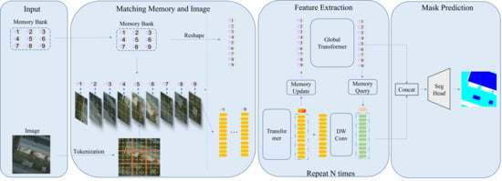
As shown in Figure 3, the main structure of the proposed model includes the local branch and the global branch. The local branch is used to extract hybrid features from the input images and the global memory tokens, while the global branch is used to encode the stored local representation into consistent global information.
Besides the two extraction branches, a DCNN encoder and a DCNN decoder are adopted to encode the image into preliminary features and to decode the features into final segmentation masks, respectively. The MAT takes the RGB image as the input and uses the encoder to extract preliminary features. Then, tokenization splits the feature space into subareas of size as in [32]. The attention scope in the local branch is thus restricted in the local size of . After the extraction of the two branches, the decoder takes both branches’ output features and fuses them into the final segmentation masks.
The extraction process is constructed in several stages with different stage settings. The extraction pipeline of a single stage is shown in Figure 4. The stage first takes the memory bank and the image feature of the former stage. Memory tokens are queried down from the and aligned with the image features. The combined representations are fed into a hybrid module for feature extraction. The image-based features are further sent into an image module to extract image features , while the memory-based feature is uploaded to the global branch by the memory update module. The memory tokens are refined in the global module by interacting with each other using the transformer.
Note that is the proposed input-invariant prior information embeddings, which are invariant to all the input images during inference.
3.3. Global Memory Guidance
Vanilla segmentation models map the input image to the final segmentation result directly. In this way, the model implicitly constructs the dataset’s information by the model parameter , which can be interpreted as , where y is the segmentation mask and x is the input image. However, in the first stage, by instantiating the contextual information as learnable features, the MAT predicts the segmentation mask under the condition of the model parameters and the learnable memory tokens m. In such a way, it can be seen as .
Besides acting as the prior information in the first stage, the memory tokens are positionally aware due to the one-to-one mapping relationship between the memory tokens and the image patches. In the subsequent feature extraction process, the memory tokens are used as the global contextual information representation, which is involved in both the global branch and the local branch. In the local branch, the memory token passes the global information to the local features and aggregates the local patch’s overall representation from the local features simultaneously.
To construct long-range information, which is essential to cluster the same objects in a different position, the global memory refinement module is proposed to refine every area’s representation (the memory token) based on other memory tokens. The memory token updated from the local aggregation module is a representation of the local patch, so the interaction between tokens can help the memory gather similar features across the whole image. The refinement strategy can strengthen the memory tokens’ representation ability by aggregating the distant instances’ information of the same classes.
The transformer is adopted as the global memory refinement module, which takes all the memory tokens as the input and extracts global information via the self-attention module and refines the single memory representation via the feedforward network.
3.4. Local Aggregation Module
The local aggregation module (Figure 5) consists of a transformer encoder and a depthwise convolution layer. The transformer encoder is used as the hybrid feature extraction module, which extracts features from the concatenated memory token and the local area features. The global receptive field of the transformer enables feature interaction between local image features and between the memory token and image features. For the image module, we adopted a single-layer depthwise convolution. The depthwise convolution was used to align the features concerning the edge point of patches and enforce some relative position information into the MAT since the transformer encoder is position invariant.
The local branch first groups the image features into several patches. Each group queries the corresponding memory token down to the link, then aligns the token with the local patches. After the alignment, these combined tokens are fed into the transformer encoders separately; all the transformer encoders share the same weight. The output feature of the transformer is split into the memory token and the image feature. The memory token is sent back into the memory bank by the memory update module. The image features are reshaped into an image grid and are further refined by a depthwise convolution to alleviate the feature misalignment on the edge of adjacent groups.
3.5. Memory-Query and Memory-Update
Bidirectional information flow between the global branch and the local branch is interleaved in every stage. The memory-query downloads the global information from the memory bank to the local module and concatenates it with the local features at the beginning of the local branch, while the memory-update passes the local aggregation information to the memory bank and replaces the original memory tokens in the bank after the local extraction.
Because of the one-to-one mapping strategy, the memory-query module only needs to query the corresponding memory token. The memory-update module is also quite simple and clear since the further refinement between memory tokens is left to the global refinement module. Both the memory-update module and the memory-query module are set as a linear layer with the GELU [58] to align the feature dimension.
3.6. Convolutional Embedding and Light Decoding Module
Following recent ViT variants [59,60] in the optical field, we used convolutional layers as the embedding module rather than directly splitting the image into several nonoverlapping patches and performing embedding in these patches. The embedding procedure is performed as,
where x is the input image of shape and is the embedded feature of . and both have a convolution layer with stride two. The only difference is that is followed by the GELU and batch norm, while only has a GELU.
Rather than U-Net, which needs a heavy decoder as the encoder to decode the features into the final segmentation mask, the MAT only uses three convolutional layers to decode the global features and local features into the final prediction. Due to the resolution-preserving nature of the transformer, our local aggregation module maintains the resolution of , only four-times downsampling of the original input resolution of . In this way, we only need a light head to perform the final segmentation prediction.
Our segmentation head utilizes both the global branch feature and the local branch feature. We first resized the global feature into the local feature’s shape, then concatenated these two features. The combined representation is decoded in the segmentation mask by a transposed convolutional layer and two convolutional layers.
4. Experiments
4.1. Experimental Details
4.1.1. Datasets
In this paper, we chose the ISPRS Potsdam and ISPRS Vaihingen datasets to evaluate our results. Below we give a brief introduction to the two datasets.
ISPRS Potsdam (https://www2.isprs.org/commissions/comm2/wg4/benchmark/2d-sem-label-potsdam/, accessed on 13 August 2021) contains 38 patches (of the same size) as Figure 6b. The images cover a large area with large variations. Each image patch consists of a True Orthophoto (TOP) extracted from a larger TOP mosaic. The ground sampling distance of the TOP is 5 cm. The dataset provides three different channel composition data. In this work, we used the RGB data to train and evaluate the MAT. We chose 28 images to train the model and the remaining 18 to test the model’s performance. The test set contained the 2_13, 2_14, 3_13, 3_14, 4_13, 4_14, 4_15, 5_13, 5_14, 5_15, 6_13, 6_14, 6_15, and 7_13 patches, which concurs with previous works [9,28,61].
ISPRS Vaihingen (https://www2.isprs.org/commissions/comm2/wg4/benchmark/2d-sem-label-vaihingen, accessed on 13 August 2021) is composed of 33 orthorectified image tiles acquired by a near-infrared (NIR)—green (G)—red (R) aerial camera, over the town of Vaihingen (Germany). The detailed images’ location and number are shown in Figure 6a. The average size of the tiles is 20,494 × 20,064 pixels with a spatial resolution of 9 cm. The dataset contains 33 patches (of different sizes), each consisting of a true orthophoto (TOP) extracted from a larger TOP mosaic. We chose 16 images to train the model and the remaining 17 to test the model’s performance. The test set contained the 2, 4, 6, 8, 10, 12, 14, 16, 20, 22, 24, 27, 29, 31, 33, 35, and 38 areas, following previous works [9,28,61].
Both datasets are provided by the International Society for Photogrammetry and Remote Sensing (ISPRS) and involve the discrimination of six land cover/land use classification classes: Impervious surfaces (Imp. surf) (roads, concrete surfaces), Buildings (Build.), Low vegetation (Low veg), trees, cars, and a class of clutter representing uncategorizable land covers.
4.1.2. Implementation Details
In both experiments, the number of memory tokens was 64 and the memory tokens’ dim was set to 128, while the dim of the local branch was 256. Three stages were adopted for feature extraction. The transformer’s depths in the local branch were set to 2, 2, and 1 for the three stages, while the transformer’s depths in the global branch were all set to 1.
For training, the images were first randomly cropped into . Such a cropping strategy resulted in a total of 12,000 training examples for ISPRS Potsdam and 8000 training examples for ISPRS Vaihingen. For the Potsdam images, we performed a random vertical flip, horizontal flip, and 90 rotation to the input image with a probability of 0.5. Then, we normalized the augmented image with a mean of (0.5, 0.5, 0.5) and an std of (1.0, 1.0, 1.0). For the Vaihingen images, we added the cutmix [62] and mixup [63] strategy and a random scale of [0.5, 2.0] due to the limited images.
The Adam optimizer was used with an initial learning rate of 0.0001, and poly-annealing as Equation (8) was adopted to decay the learning rate in the training process, where is the initial learning rate, and denote the current iteration and the total iterations of the experiment, and is a hyperparameter set to 0.5 by default. We also used warm-up [64] for the first 100 iterations. All experiments only used the cross-entropy loss without additional loss, such as focal loss or Dice loss.
For testing, a slide image prediction strategy was adopted, and the metric is reported concerning the original image size. Normalization was the only augmentation used during inference. The cropping image size was set to 512, and the cropping stride was set to 200, which led to 312 overlaps for adjacent image crops.
All experiments were carried out on a single NVIDIA V100 with 4 images every batch and 100 training epochs.
4.2. Evaluation Metrics
We report the mean Intersection over Union (mIoU) and average F1-score in the following experiments.
The mIoU score is calculated as follows, which is the average of all class’s IoU:
where N is the total number of the classes and , , and are short for True Positive, False Positive, and False Negative, respectively. Footnote i denotes the i-th ground truth class.
The AF score’s calculation process is as follows.
where P and R are short for Precision and Recall and subscript i denotes the i-th ground truth class.
4.3. Results
For the experiments, we report the five foreground classes’ F1-score and their average F1-score and mIoU, as in the previous works [9,10,28]. The results on the Potsdam datasets are reported in Table 1. The MAT achieved an average F1-score of 91.59 and an mIoU of 84.82, which all outperformed previous DCNN-based works.
4.4. Ablation Study
Several ablation experiments were carried out on the architectures to verify the effectiveness of the proposed module.
4.4.1. Memory Prior
The performance of the memory prior was measured by setting a control experiment. The memory prior denotes the memory tokens in the first stage where they are learned to encode beneficial information for the segmentation tasks. Memory tokens were set to zero compared with the original work. In such a setting, the memory bank only serves as a global information representation, and it encodes zero input-invariant prior information due to its zero initialization. Moreover, to see whether the memory encodes the location-invariant contextual information or location-variant information, the learned memory priors were visualized using T-SNE [72]. If they encoded location-invariant information, the visualization result tended to form a single cluster. On the contrary, if they encoded location-variant information, the visualization result tended to scatter in the whole picture.
4.4.2. Global Branch
As for the global information branch, we verified its effectiveness by comparing the model’s performance with the global branch and without the global branch. By removing the global branch, the memory bank was also removed. The MAT only had the local branch, which consisted of the transformer and the depthwise convolution. The final segmentation mask was predicted by the image feature only.
4.4.3. Ablation Results
The ablation results are reported in Table 3. Without the memory prior and directly setting the memory bank to zero at the beginning of the inference, the mIoU and average F1-score dropped for both datasets. For the Potsdam dataset, the mIoU dropped and the average F1-score dropped . For the Vaihingen dataset, the mIoU dropped and the average F1-score dropped . After removing the global branch, the model uses the transformer and depthwise convolution to extract features and perform the prediction. The mIoU and average F1-score on the Potsdam dataset dropped and , respectively, while they dropped and on the Vaihingen dataset, respectively.
The T-SNE visualization results are shown in Figure 7, and each point represents a single memory token in the memory bank. The memory prior tokens are scattered across the whole plane, which means they provide different prior information at the beginning of the inference stage.
5. Discussion
The experiment results demonstrated that the MAT, which facilitates both the prior information and the input-based representation, performs well in high-resolution remote sensing image semantic segmentation tasks. Noted that the MAT only has M parameters, which is comparably smaller than DCNNs, whose encoder backbones are mainly VGG16 with M parameters and ResNet101 with M parameters.
For the Potsdam dataset, the MAT outperformed previous methods in the overall metrics and in F1-scores of all the classes, which demonstrated the MAT’s effectiveness in handling high-resolution remote sensing image semantic segmentation tasks. The MAT achieved an average F1-score of 91.59 and an mIoU of 84.82. As for the comparison, the attention-aided method S-RA-FCN, which adopts VGG16 as the backbone, appends heavy feature fusion modules in the decoder, and uses multiple loss to train the network, only obtained an average of a 90.17 F1-score and an mIoU of 82.38. The MAT outperformed the S-RA-FCN mostly in classes that tended to occupy large areas such as impervious surface ( F1-score) and building ( F1-score) due to the benefit of the large receptive field of the transformer and the explicit global branch. The total gains in the average F1-score were and for the mIoU .
For the Vaihingen dataset, the results reported in Table 2 show that the MAT’s performance was competitive with the S-RA-FCN, while it could surpass other works by a large margin.
The superior performance of the MAT can be largely attributed to the powerful representation ability of the transformer, which can extract global information from all the locations in the image. The memory mechanism can decouple the extraction process into local feature extraction and global information guidance, which can ease the computational complexity of the transformer and avoid optimizing overly long image patches.
The segmentation results of the MAT and FCN8s are presented in Figure 8 and Figure 9 for a visual comparison. The first row is the input remote sensing images, the second row the ground truth segmentation masks, the third row the prediction of the FCN8s, which was trained using the same hyperparameters as the MAT, and the last row the MAT’s prediction. The results showed that the MAT can surpass the FCN in most cases. The MAT can better capture the primary structure of the target and locate the boundaries between targets and small objects such as cars. Especially on the Vaihingen dataset, as shown in Figure 9, the FCN tended to predict more clutters and to wrongly classify instances. On the contrary, the MAT performed much better than the FCN8s, being able to segment the images holistically concurrently with ground truth.
Besides cropping image visualization, the segmentation results of the sliding image inference strategy are also provided. The visualization results were cropped from the whole prediction mask, and the cropping size was 1000 × 1000. As shown in Figure 10, after the slide inference, both the FCN and MAT performed better compared with the direct inference result in Figure 8 and Figure 9.
The FCN tended to predict smoothed masks that would miss the intervals between objects and small objects that are surrounded by other classes. To be specific, the FCN’s prediction missed many cars in the third image of the Potsdam dataset, eroded all the intervals between the low vegetation into the low vegetation class in the second image of the Potsdam dataset, and neglected all the clutter class in the first and last images of the Potsdam dataset.
As for the result on the Vaihingen dataset, the false predictions of the FCN were greatly suppressed, but its quality was still lower compared to the results of the MAT. The results of the FCN were so smooth that it was difficult to locate the corners of the buildings. For cars that mainly lie inside the impervious surface, the FCN tended to ignore them, while the MAT perfectly segmented it out.
The ablation study in Table 3 verified the effectiveness of the proposed memory prior and the global module. Note that the experiment without the global module did not have the memory prior. The experimental results showed that the results reported on the model without the global module were inferior to the model without the memory prior. It can be delineated that the global module and the memory prior are reciprocal since with both of them, the results were far better than adopting only one.
The T-SNE results of the learned prior on both datasets are shown in Figure 7. The visualization results showed that these tokens tended to learn different memory prior information concerning their locations. Moreover, the ablation study in Table 3 confirmed that the memory prior could obtain a mIoU gain and a average F1-score gain on the Potsdam dataset, while it could obtain a mIoU gain and a average F1-score gain on the Vaihingen dataset.
However, the limitations of the MAT are mainly two fold. Firstly, the quadratic computation complexity of self-attention with respect to the input token number of the transformer encoder still made the MAT’s MACs higher even if the transformer had a relatively smaller number of model parameters. For example, the MAC of our model was G for an image of size ; therefore, it is worth exploring the use of more efficient transformer variants to reduce the computation, and we leave this for future works. Secondly, the transformer encoder augments the global information representation ability at the expense of local continuity, which sometimes made our semantic results tend to be cluttered, especially in small areas and edges. Detailed cases are shown in Figure 11, where our methods were not smooth enough in the first two segmentations and small noise areas were intersected with the main object in the last image.
6. Conclusions
In this paper, a memory-augmented transformer model was proposed to perform high-resolution remote sensing image semantic segmentation tasks. Prior information was added to the network via learnable memory tokens. A global branch and a local branch were proposed for parallel feature extraction. Memory-query and memory-update were interleaved between the two branches to facilitate information interaction between the global and local branch. We used the transformer encoder as the base feature extraction module to aggregate local information between spatial features and global information between memory tokens. Experimental results showed that our method can achieve comparable accuracies to the SOTA methods.
Author Contributions
Conceptualization, X.Z.; Methodology, X.Z. and J.G.; Supervision, Y.W.; Validation, Y.Z. All authors have read and agreed to the published version of the manuscript.
Funding
The work in this paper is supported by the National Key R&D Program of China (2018YFC1407201).
Institutional Review Board Statement
Not applicable.
Informed Consent Statement
Not applicable.
Data Availability Statement
The datasets used in this work can be accessed at https://www2.isprs.org/commissions/comm2/wg4/benchmark/data-request-form, accessed on 13 August 2021.
Conflicts of Interest
The authors declare no conflict of interest.
Abbreviations
The following abbreviations are used in this manuscript:
| DCNN | Deep convolutional neural network |
| MAT | Memory-augmented transformer |
| ViT | Vision transformer |
| NLP | Natural language processing |
| GELUs | Gaussian error linear units |
References
- Neupane, B.; Horanont, T.; Aryal, J. Deep Learning-Based Semantic Segmentation of Urban Features in Satellite Images: A Review and Meta-Analysis. Remote Sens. 2021, 13, 808. [Google Scholar] [CrossRef]
- Yuan, X.; Shi, J.; Gu, L. A review of deep learning methods for semantic segmentation of remote sensing imagery. Expert Syst. Appl. 2021, 169, 114417. [Google Scholar] [CrossRef]
- Lateef, F.; Ruichek, Y. Survey on semantic segmentation using deep learning techniques. Neurocomputing 2019, 338, 321–348. [Google Scholar] [CrossRef]
- Grinias, I.; Panagiotakis, C.; Tziritas, G. MRF-based segmentation and unsupervised classification for building and road detection in peri-urban areas of high-resolution satellite images. ISPRS J. Photogramm. Remote Sens. 2016, 122, 145–166. [Google Scholar] [CrossRef]
- Huang, X.; Zhang, L.; Gong, W. Information fusion of aerial images and LIDAR data in urban areas: Vector-stacking, re-classification and post-processing approaches. Int. J. Remote Sens. 2011, 32, 69–84. [Google Scholar] [CrossRef]
- Yang, Y.; Hallman, S.; Ramanan, D.; Fowlkes, C.C. Layered object models for image segmentation. IEEE Trans. Pattern Anal. Mach. Intell. 2011, 34, 1731–1743. [Google Scholar] [CrossRef] [Green Version]
- Schiefer, F.; Kattenborn, T.; Frick, A.; Frey, J.; Schall, P.; Koch, B.; Schmidtlein, S. Mapping forest tree species in high resolution UAV-based RGB-imagery by means of convolutional neural networks. ISPRS J. Photogramm. Remote Sens. 2020, 170, 205–215. [Google Scholar] [CrossRef]
- Nezami, S.; Khoramshahi, E.; Nevalainen, O.; Pölönen, I.; Honkavaara, E. Tree species classification of drone hyperspectral and rgb imagery with deep learning convolutional neural networks. Remote Sens. 2020, 12, 1070. [Google Scholar] [CrossRef] [Green Version]
- Mou, L.; Hua, Y.; Zhu, X.X. A relation-augmented fully convolutional network for semantic segmentation in aerial scenes. In Proceedings of the IEEE/CVF Conference on Computer Vision and Pattern Recognition, Long Beach, CA, USA, 15–20 June 2019; pp. 12416–12425. [Google Scholar]
- Peng, C.; Zhang, K.; Ma, Y.; Ma, J. Cross Fusion Net: A Fast Semantic Segmentation Network for Small-Scale Semantic Information Capturing in Aerial Scenes. IEEE Trans. Geosci. Remote. Sens. 2021. [Google Scholar] [CrossRef]
- Chen, L.C.; Papandreou, G.; Schroff, F.; Adam, H. Rethinking atrous convolution for semantic image segmentation. arXiv 2017, arXiv:1706.05587. [Google Scholar]
- Chen, L.C.; Papandreou, G.; Kokkinos, I.; Murphy, K.; Yuille, A.L. Deeplab: Semantic image segmentation with deep convolutional nets, atrous convolution, and fully connected crfs. IEEE Trans. Pattern Anal. Mach. Intell. 2017, 40, 834–848. [Google Scholar] [CrossRef] [PubMed]
- Yuan, Y.; Huang, L.; Guo, J.; Zhang, C.; Chen, X.; Wang, J. Ocnet: Object context network for scene parsing. arXiv 2018, arXiv:1809.00916. [Google Scholar]
- Tao, A.; Sapra, K.; Catanzaro, B. Hierarchical multi-scale attention for semantic segmentation. arXiv 2020, arXiv:2005.10821. [Google Scholar]
- Dai, J.; Qi, H.; Xiong, Y.; Li, Y.; Zhang, G.; Hu, H.; Wei, Y. Deformable convolutional networks. In Proceedings of the IEEE International Conference on Computer Vision, Venice, Italy, 22–29 October 2017; pp. 764–773. [Google Scholar]
- Zhu, X.; Hu, H.; Lin, S.; Dai, J. Deformable convnets v2: More deformable, better results. In Proceedings of the IEEE/CVF Conference on Computer Vision and Pattern Recognition, Long Beach, CA, USA, 15–20 June 2019; pp. 9308–9316. [Google Scholar]
- Vaswani, A.; Shazeer, N.; Parmar, N.; Uszkoreit, J.; Jones, L.; Gomez, A.N.; Kaiser, Ł.; Polosukhin, I. Attention is all you need. In Proceedings of the Advances in Neural Information Processing Systems, Long Beach, CA, USA, 4–9 December 2017; pp. 5998–6008. [Google Scholar]
- Blaschke, T.; Hay, G.J.; Kelly, M.; Lang, S.; Hofmann, P.; Addink, E.; Feitosa, R.Q.; Van der Meer, F.; Van der Werff, H.; Van Coillie, F.; et al. Geographic object-based image analysis–towards a new paradigm. ISPRS J. Photogramm. Remote Sens. 2014, 87, 180–191. [Google Scholar] [CrossRef] [PubMed] [Green Version]
- Derivaux, S.; Lefevre, S.; Wemmert, C.; Korczak, J. Watershed segmentation of remotely sensed images based on a supervised fuzzy pixel classification. In Proceedings of the IEEE International Geosciences And Remote Sensing Symposium (IGARSS), Denver, CO, USA, 31 July–4 August 2006; pp. 3712–3715. [Google Scholar]
- Su, T. Scale-variable region-merging for high resolution remote sensing image segmentation. ISPRS J. Photogramm. Remote Sens. 2019, 147, 319–334. [Google Scholar] [CrossRef]
- Pesaresi, M.; Benediktsson, J.A. A new approach for the morphological segmentation of high-resolution satellite imagery. IEEE Trans. Geosci. Remote Sens. 2001, 39, 309–320. [Google Scholar] [CrossRef] [Green Version]
- Chehata, N.; Orny, C.; Boukir, S.; Guyon, D.; Wigneron, J. Object-based change detection in wind storm-damaged forest using high-resolution multispectral images. Int. J. Remote Sens. 2014, 35, 4758–4777. [Google Scholar] [CrossRef]
- Long, J.; Shelhamer, E.; Darrell, T. Fully convolutional networks for semantic segmentation. In Proceedings of the IEEE Conference on Computer Vision and Pattern Recognition, Boston, MA, USA, 7–12 June 2015; pp. 3431–3440. [Google Scholar]
- Ronneberger, O.; Fischer, P.; Brox, T. U-net: Convolutional networks for biomedical image segmentation. In Proceedings of the International Conference on Medical Image Computing and Computer-Assisted Intervention, Munich, Germany, 5–9 October 2015; pp. 234–241. [Google Scholar]
- Qiu, C.; Schmitt, M.; Geiß, C.; Chen, T.H.K.; Zhu, X.X. A framework for large-scale mapping of human settlement extent from Sentinel-2 images via fully convolutional neural networks. ISPRS J. Photogramm. Remote Sens. 2020, 163, 152–170. [Google Scholar] [CrossRef]
- Fu, T.; Ma, L.; Li, M.; Johnson, B.A. Using convolutional neural network to identify irregular segmentation objects from very high-resolution remote sensing imagery. J. Appl. Remote Sens. 2018, 12, 025010. [Google Scholar] [CrossRef]
- Ding, L.; Zhang, J.; Bruzzone, L. Semantic segmentation of large-size VHR remote sensing images using a two-stage multiscale training architecture. IEEE Trans. Geosci. Remote Sens. 2020, 58, 5367–5376. [Google Scholar] [CrossRef]
- Li, H.; Qiu, K.; Chen, L.; Mei, X.; Hong, L.; Tao, C. SCAttNet: Semantic segmentation network with spatial and channel attention mechanism for high-resolution remote sensing images. IEEE Geosci. Remote Sens. Lett. 2020, 18, 905–909. [Google Scholar] [CrossRef]
- Burtsev, M.S.; Kuratov, Y.; Peganov, A.; Sapunov, G.V. Memory transformer. arXiv 2020, arXiv:2006.11527. [Google Scholar]
- Carion, N.; Massa, F.; Synnaeve, G.; Usunier, N.; Kirillov, A.; Zagoruyko, S. End-to-end object detection with transformers. In Proceedings of the European Conference on Computer Vision, Glasgow, UK, 23–28 August 2020; pp. 213–229. [Google Scholar]
- Zhu, X.; Su, W.; Lu, L.; Li, B.; Wang, X.; Dai, J. Deformable detr: Deformable transformers for end-to-end object detection. arXiv 2020, arXiv:2010.04159. [Google Scholar]
- Dosovitskiy, A.; Beyer, L.; Kolesnikov, A.; Weissenborn, D.; Zhai, X.; Unterthiner, T.; Dehghani, M.; Minderer, M.; Heigold, G.; Gelly, S.; et al. An image is worth 16x16 words: Transformers for image recognition at scale. arXiv 2020, arXiv:2010.11929. [Google Scholar]
- Liu, Z.; Lin, Y.; Cao, Y.; Hu, H.; Wei, Y.; Zhang, Z.; Lin, S.; Guo, B. Swin transformer: Hierarchical vision transformer using shifted windows. arXiv 2021, arXiv:2103.14030. [Google Scholar]
- Wang, W.; Xie, E.; Li, X.; Fan, D.P.; Song, K.; Liang, D.; Lu, T.; Luo, P.; Shao, L. Pyramid vision transformer: A versatile backbone for dense prediction without convolutions. arXiv 2021, arXiv:2102.12122. [Google Scholar]
- Chu, X.; Tian, Z.; Wang, Y.; Zhang, B.; Ren, H.; Wei, X.; Xia, H.; Shen, C. Twins: Revisiting the design of spatial attention in vision transformers. arXiv 2021, arXiv:2104.13840. [Google Scholar]
- Sun, P.; Jiang, Y.; Zhang, R.; Xie, E.; Cao, J.; Hu, X.; Kong, T.; Yuan, Z.; Wang, C.; Luo, P. Transtrack: Multiple-object tracking with transformer. arXiv 2020, arXiv:2012.15460. [Google Scholar]
- Yan, B.; Peng, H.; Fu, J.; Wang, D.; Lu, H. Learning spatio-temporal transformer for visual tracking. arXiv 2021, arXiv:2103.17154. [Google Scholar]
- Hirose, S.; Wada, N.; Katto, J.; Sun, H. ViT-GAN: Using Vision Transformer as Discriminator with Adaptive Data Augmentation. In Proceedings of the 2021 3rd International Conference on Computer Communication and the Internet (ICCCI), Nagoya, Japan, 25–27 June 2021; pp. 185–189. [Google Scholar]
- Lee, K.; Chang, H.; Jiang, L.; Zhang, H.; Tu, Z.; Liu, C. ViTGAN: Training GANs with Vision Transformers. arXiv 2021, arXiv:2107.04589. [Google Scholar]
- Esser, P.; Rombach, R.; Ommer, B. Taming transformers for high-resolution image synthesis. In Proceedings of the IEEE/CVF Conference on Computer Vision and Pattern Recognition, Nashville, TN, USA, 19–25 June 2021; pp. 12873–12883. [Google Scholar]
- Engel, N.; Belagiannis, V.; Dietmayer, K. Point transformer. arXiv 2020, arXiv:2011.00931. [Google Scholar]
- Guo, M.H.; Cai, J.X.; Liu, Z.N.; Mu, T.J.; Martin, R.R.; Hu, S.M. PCT: Point cloud transformer. arXiv 2020, arXiv:2012.09688. [Google Scholar]
- Qing, Y.; Liu, W.; Feng, L.; Gao, W. Improved Transformer Net for Hyperspectral Image Classification. Remote Sens. 2021, 13, 2216. [Google Scholar] [CrossRef]
- Bazi, Y.; Bashmal, L.; Rahhal, M.M.A.; Dayil, R.A.; Ajlan, N.A. Vision Transformers for Remote Sensing Image Classification. Remote Sens. 2021, 13, 516. [Google Scholar] [CrossRef]
- He, X.; Chen, Y.; Lin, Z. Spatial-Spectral Transformer for Hyperspectral Image Classification. Remote Sens. 2021, 13, 498. [Google Scholar] [CrossRef]
- Li, W.; Cao, D.; Peng, Y.; Yang, C. MSNet: A Multi-Stream Fusion Network for Remote Sensing Spatiotemporal Fusion Based on Transformer and Convolution. Remote Sens. 2021, 13, 3724. [Google Scholar] [CrossRef]
- Yu, Y.; Zhao, J.; Gong, Q.; Huang, C.; Zheng, G.; Ma, J. Real-Time Underwater Maritime Object Detection in Side-Scan Sonar Images Based on Transformer-YOLOv5. Remote Sens. 2021, 13, 3555. [Google Scholar] [CrossRef]
- Xu, Z.; Zhang, W.; Zhang, T.; Yang, Z.; Li, J. Efficient Transformer for Remote Sensing Image Segmentation. Remote Sens. 2021, 13, 3585. [Google Scholar] [CrossRef]
- Wang, L.; Li, R.; Wang, D.; Duan, C.; Wang, T.; Meng, X. Transformer Meets Convolution: A Bilateral Awareness Network for Semantic Segmentation of Very Fine Resolution Urban Scene Images. Remote Sens. 2021, 13, 3065. [Google Scholar] [CrossRef]
- Oord, A.V.D.; Vinyals, O.; Kavukcuoglu, K. Neural discrete representation learning. arXiv 2017, arXiv:1711.00937. [Google Scholar]
- Razavi, A.; van den Oord, A.; Vinyals, O. Generating diverse high-fidelity images with vq-vae-2. In Proceedings of the Advances in Neural Information Processing Systems, Vancouver, QC, Canada, 8–14 December 2019; pp. 14866–14876. [Google Scholar]
- Han, T.; Xie, W.; Zisserman, A. Memory-augmented dense predictive coding for video representation learning. In Proceedings of the Computer Vision–ECCV 2020: 16th European Conference, Glasgow, UK, 23–28 August 2020; pp. 312–329. [Google Scholar]
- Oh, S.W.; Lee, J.Y.; Xu, N.; Kim, S.J. Video object segmentation using space-time memory networks. In Proceedings of the IEEE/CVF International Conference on Computer Vision, Long Beach, CA, USA, 16–17 June 2019; pp. 9226–9235. [Google Scholar]
- Gong, D.; Liu, L.; Le, V.; Saha, B.; Mansour, M.R.; Venkatesh, S.; Hengel, A.V.D. Memorizing normality to detect anomaly: Memory-augmented deep autoencoder for unsupervised anomaly detection. In Proceedings of the IEEE/CVF International Conference on Computer Vision, Long Beach, CA, USA, 16–17 June 2019; pp. 1705–1714. [Google Scholar]
- Kim, Y.; Kim, M.; Kim, G. Memorization precedes generation: Learning unsupervised gans with memory networks. arXiv 2018, arXiv:1803.01500. [Google Scholar]
- Santoro, A.; Bartunov, S.; Botvinick, M.; Wierstra, D.; Lillicrap, T. Meta-learning with memory-augmented neural networks. In Proceedings of the International Conference on Machine Learning, New York, NY, USA, 20–22 June 2016; pp. 1842–1850. [Google Scholar]
- Guo, M.H.; Liu, Z.N.; Mu, T.J.; Hu, S.M. Beyond self-attention: External attention using two linear layers for visual tasks. arXiv 2021, arXiv:2105.02358. [Google Scholar]
- Hendrycks, D.; Gimpel, K. Gaussian Error Linear Units (GELUs). arXiv 2020, arXiv:1606.08415. [Google Scholar]
- Vaswani, A.; Ramachandran, P.; Srinivas, A.; Parmar, N.; Hechtman, B.; Shlens, J. Scaling local self-attention for parameter efficient visual backbones. In Proceedings of the IEEE/CVF Conference on Computer Vision and Pattern Recognition, Nashville, TN, USA, 19–25 June 2021; pp. 12894–12904. [Google Scholar]
- Wu, H.; Xiao, B.; Codella, N.; Liu, M.; Dai, X.; Yuan, L.; Zhang, L. Cvt: Introducing convolutions to vision transformers. arXiv 2021, arXiv:2103.15808. [Google Scholar]
- Niu, R.; Sun, X.; Tian, Y.; Diao, W.; Chen, K.; Fu, K. Hybrid multiple attention network for semantic segmentation in aerial images. IEEE Trans. Geosci. Remote Sens. 2021. [Google Scholar] [CrossRef]
- Yun, S.; Han, D.; Oh, S.J.; Chun, S.; Choe, J.; Yoo, Y. Cutmix: Regularization strategy to train strong classifiers with localizable features. In Proceedings of the IEEE/CVF International Conference on Computer Vision, Long Beach, CA, USA, 16–17 June 2019; pp. 6023–6032. [Google Scholar]
- Zhang, H.; Cisse, M.; Dauphin, Y.N.; Lopez-Paz, D. mixup: Beyond empirical risk minimization. arXiv 2017, arXiv:1710.09412. [Google Scholar]
- He, K.; Zhang, X.; Ren, S.; Sun, J. Deep residual learning for image recognition. In Proceedings of the IEEE Conference on Computer Vision and Pattern Recognition, Las Vegas, NV, USA, 27–30 June 2016; pp. 770–778. [Google Scholar]
- Pan, X.; Shi, J.; Luo, P.; Wang, X.; Tang, X. Spatial as deep: Spatial cnn for traffic scene understanding. In Proceedings of the Thirty-Second AAAI Conference on Artificial Intelligence, New Orleans, LA, USA, 2–7 February 2018. [Google Scholar]
- Sun, Y.; Zhang, X.; Xin, Q.; Huang, J. Developing a multi-filter convolutional neural network for semantic segmentation using high-resolution aerial imagery and LiDAR data. ISPRS J. Photogramm. Remote Sens. 2018, 143, 3–14. [Google Scholar] [CrossRef]
- Volpi, M.; Tuia, D. Dense semantic labeling of subdecimeter resolution images with convolutional neural networks. IEEE Trans. Geosci. Remote Sens. 2016, 55, 881–893. [Google Scholar] [CrossRef] [Green Version]
- Nogueira, K.; Dalla Mura, M.; Chanussot, J.; Schwartz, W.R.; Dos Santos, J.A. Dynamic multicontext segmentation of remote sensing images based on convolutional networks. IEEE Trans. Geosci. Remote Sens. 2019, 57, 7503–7520. [Google Scholar] [CrossRef] [Green Version]
- Shi, H.; Fan, J.; Wang, Y.; Chen, L. Dual Attention Feature Fusion and Adaptive Context for Accurate Segmentation of Very High-Resolution Remote Sensing Images. Remote Sens. 2021, 13, 3715. [Google Scholar] [CrossRef]
- Marcos, D.; Volpi, M.; Kellenberger, B.; Tuia, D. Land cover mapping at very high resolution with rotation equivariant CNNs: Towards small yet accurate models. ISPRS J. Photogramm. Remote Sens. 2018, 145, 96–107. [Google Scholar] [CrossRef] [Green Version]
- Chai, D.; Newsam, S.; Huang, J. Aerial image semantic segmentation using DCNN predicted distance maps. ISPRS J. Photogramm. Remote Sens. 2020, 161, 309–322. [Google Scholar] [CrossRef]
- Van der Maaten, L.; Hinton, G. Visualizing data using t-SNE. J. Mach. Learn. Res. 2008, 9, 2579–2605. [Google Scholar]
Figure 1.
The paradigm of the semantic segmentation pipeline. Most works adopt an encoder–decoder structure such as (a), where X is the input image and Y is the predicted segmentation mask. In (b), the model learns to predict the segmentation mask based on both the input image and the memory m. Memory is used to help encode some contextual information of the dataset and is learned along with the model parameters. Skip connections between the encoder and decoder are omitted in the figure for simplicity.

Figure 2.
Structure of the transformer encoder. (a) The transformer encoder mainly consists of a multi-head attention module, a feedforward network (FFN), and two residual connections. (b) The multi-head attention first projects the input x into three vectors of the same shape, which are called the query, key, and value. The module then calculates the similarity coefficients between the query and the key vector. The similarity values are used as attention scores. The attention scores are further used to calculate the weighted sum of the value vector. (c) The FFN expands the input x into a higher dim and squeezes it back using an MLP. A nonlinear layer such as GELU [58] is inserted between the two fully connected layers.

Figure 3.
The proposed model for remote sensing segmentation. The MAT mainly consists of a global branch and a local branch. The global branch refines the memory bank, which is used as a representation of the prior and global information. The local branch extracts features from the input images. Bidirectional information flow between the two branches is enforced by the memory-query and memory-update modules. Then, the two branches’ output representation is fed into the segmentation head to perform segmentation prediction.

Figure 4.
The extraction process of a single stage. denotes the output memory token and image features of the i-th stage.
Figure 4.
The extraction process of a single stage. denotes the output memory token and image features of the i-th stage.

Figure 5.
Local aggregation module’s structure. The input image features are first to split into different patches, then the corresponding memory tokens are queried from the global branch and appended as a token along with the features. All the patches are passed through a transformer encoder for feature extraction. These features are reshaped back to image grids and fed into a depthwise convolution layer for local feature alignment. Note that the weight sharing strategy is used in all transformers for parameter efficiency consideration.

Figure 6.
The detailed image patch location and corresponding number of the Potsdam and Vaihingen datasets.
Figure 6.
The detailed image patch location and corresponding number of the Potsdam and Vaihingen datasets.

Figure 7.
The T-SNE results of the memory prior. Different memory tends to encode different features due to the scattered distribution of the visualization results.
Figure 7.
The T-SNE results of the memory prior. Different memory tends to encode different features due to the scattered distribution of the visualization results.

Figure 8.
The 512 × 512 segmentation results on the Potsdam dataset. The FCN results are predicted by our implementation in the same hyperparameter settings, and the annotation colors are consistent with the ground truth.
Figure 8.
The 512 × 512 segmentation results on the Potsdam dataset. The FCN results are predicted by our implementation in the same hyperparameter settings, and the annotation colors are consistent with the ground truth.

Figure 9.
The 512 × 512 segmentation results on the Vaihingen dataset. The FCN results are predicted by our implementation in the same hyperparameter settings, and the annotation colors are consistent with the ground truth.
Figure 9.
The 512 × 512 segmentation results on the Vaihingen dataset. The FCN results are predicted by our implementation in the same hyperparameter settings, and the annotation colors are consistent with the ground truth.

Figure 10.
Segmentation results on the two datasets using the slide inference strategy. The result are cropped from the original image prediction: (a) 1000 × 1000 segmentation results on the Potsdam dataset; (b) 1000 × 1000 segmentation results on the Vaihingen dataset.
Figure 10.
Segmentation results on the two datasets using the slide inference strategy. The result are cropped from the original image prediction: (a) 1000 × 1000 segmentation results on the Potsdam dataset; (b) 1000 × 1000 segmentation results on the Vaihingen dataset.

Figure 11.
The failure cases of our proposed model. The failure parts are highlighted by the dashed yellow box, and the zoomed results are appended to the top right corner for better visualization.
Figure 11.
The failure cases of our proposed model. The failure parts are highlighted by the dashed yellow box, and the zoomed results are appended to the top right corner for better visualization.


Table 1.
Comparison with state-of-the-art methods on the Potsdam dataset. Bold type indicates the best performance.
Table 1.
Comparison with state-of-the-art methods on the Potsdam dataset. Bold type indicates the best performance.
| Model Name | Imp. Surf | Build. | Low veg | Tree | Car | Average F1 | mIoU |
|---|---|---|---|---|---|---|---|
| SCAttNet V1 [28] | 82.01 | 87.26 | 80.03 | 76.92 | 86.49 | 82.54 | 70.47 |
| SCNN [65] | 88.37 | 92.32 | 83.68 | 80.94 | 91.17 | 84.22 | 77.72 |
| Multi-filter CNN [66] | 90.94 | 96.98 | 76.32 | 73.37 | 88.55 | 85.23 | - |
| UZ_1 [67] | 89.30 | 95.40 | 81.80 | 80.50 | 86.50 | 86.70 | - |
| FCN [23] | 88.61 | 93.29 | 83.29 | 79.83 | 93.02 | 87.61 | 78.34 |
| SCAttNet V2 [28] | 90.04 | 94.05 | 84.05 | 79.75 | 89.06 | 87.39 | 77.94 |
| UFMG_4 [68] | 90.80 | 95.60 | 84.40 | 84.30 | 92.40 | 89.50 | - |
| S-RA-FCN [9] | 91.33 | 94.70 | 86.81 | 83.47 | 94.52 | 90.17 | 82.38 |
| CF-Net (ResNet-18) [10] | 90.95 | 93.19 | 86.19 | 84.49 | 95.53 | 90.07 | 82.29 |
| CF-Net (VGG-16) [10] | 90.88 | 94.18 | 86.51 | 84.73 | 95.53 | 90.37 | 82.69 |
| MAT | 93.48 | 96.04 | 86.80 | 85.35 | 96.28 | 91.59 | 84.82 |
Table 2.
Comparison with state-of-the-art methods on the Vaihingen dataset. Bold type indicates the best performance.
Table 2.
Comparison with state-of-the-art methods on the Vaihingen dataset. Bold type indicates the best performance.
| Model Name | Imp. Surf | Build. | Low Veg | Tree | Car | Average F1 | mIoU |
|---|---|---|---|---|---|---|---|
| DAFFM+ACAM [69] | 80.11 | 86.57 | 65.56 | 76.24 | 66.64 | 75.02 | - |
| UZ_1 [67] | 89.29 | 92.50 | 81.60 | 86.90 | 57.30 | 81.50 | - |
| SCAttNet V1 [28] | 87.36 | 89.54 | 77.30 | 79.16 | 69.86 | 81.23 | 68.99 |
| SCAttNet V2 [28] | 89.13 | 90.30 | 80.04 | 80.31 | 70.50 | 82.52 | 70.77 |
| FCN [23] | 88.67 | 92.83 | 76.32 | 86.67 | 74.21 | 83.74 | 72.69 |
| RoteEqNet [70] | 89.50 | 94.80 | 77.50 | 86.50 | 72.60 | 84.18 | - |
| SCNN [65] | 88.21 | 91.80 | 77.17 | 87.23 | 78.60 | 84.40 | 73.73 |
| U-Net [24] | 89.82 | 92.49 | 78.86 | 87.86 | 80.84 | 85.97 | 75.76 |
| SegNet+Distance maps [71] | 91.47 | 94.76 | 81.91 | 88.49 | 74.01 | 86.12 | - |
| UFMG_4 [68] | 91.10 | 94.50 | 82.90 | 88.80 | 81.30 | 87.72 | - |
| S-RA-FCN [9] | 91.47 | 94.97 | 80.63 | 88.57 | 87.05 | 88.54 | 79.76 |
| MAT | 91.89 | 94.14 | 83.36 | 89.03 | 85.07 | 88.70 | 79.93 |
Table 3.
Ablation results on the Potsdam and Vaihingen datasets. w/o Mem Prior denotes the model without the memory prior, and w/o G Module denotes the model without the global branch. Bold type indicates the best performance.
Table 3.
Ablation results on the Potsdam and Vaihingen datasets. w/o Mem Prior denotes the model without the memory prior, and w/o G Module denotes the model without the global branch. Bold type indicates the best performance.
| Method | Potsdam | Vaihingen | ||
|---|---|---|---|---|
| mIoU | Average F1 | mIoU | Average F1 | |
| w/o Mem Prior | 82.62 | 90.24 | 76.38 | 86.41 |
| w/o G Module | 82.58 | 90.21 | 75.31 | 85.66 |
| MAT | 84.82 | 91.59 | 79.93 | 88.70 |
Publisher’s Note: MDPI stays neutral with regard to jurisdictional claims in published maps and institutional affiliations. |
© 2021 by the authors. Licensee MDPI, Basel, Switzerland. This article is an open access article distributed under the terms and conditions of the Creative Commons Attribution (CC BY) license (https://creativecommons.org/licenses/by/4.0/).
Share and Cite
MDPI and ACS Style
Zhao, X.; Guo, J.; Zhang, Y.; Wu, Y. Memory-Augmented Transformer for Remote Sensing Image Semantic Segmentation. Remote Sens. 2021, 13, 4518. https://doi.org/10.3390/rs13224518
AMA Style
Zhao X, Guo J, Zhang Y, Wu Y. Memory-Augmented Transformer for Remote Sensing Image Semantic Segmentation. Remote Sensing. 2021; 13(22):4518. https://doi.org/10.3390/rs13224518
Chicago/Turabian StyleZhao, Xin, Jiayi Guo, Yueting Zhang, and Yirong Wu. 2021. "Memory-Augmented Transformer for Remote Sensing Image Semantic Segmentation" Remote Sensing 13, no. 22: 4518. https://doi.org/10.3390/rs13224518
Note that from the first issue of 2016, this journal uses article numbers instead of page numbers. See further details here.