
Accelerated Multi-View Stereo for 3D Reconstruction of Transmission Corridor with Fine-Scale Power Line


1
State Key Laboratory of Information Engineering in Surveying, Mapping and Remote Sensing, Wuhan University, 129 Luoyu Road, Wuhan 430079, China
2
School of Computer Science, China University of Geosciences, Wuhan 430074, China
3
Collaborative Innovation Center of Geospatial Technology, Wuhan University, 129 Luoyu Road, Wuhan 430079, China
*
Author to whom correspondence should be addressed.
Remote Sens. 2021, 13(20), 4097; https://doi.org/10.3390/rs13204097
Submission received: 10 September 2021
/
Revised: 8 October 2021
/
Accepted: 9 October 2021
/
Published: 13 October 2021
(This article belongs to the Special Issue Techniques and Applications of UAV-Based Photogrammetric 3D Mapping)
Abstract
:Fast reconstruction of power lines and corridors is a critical task in UAV (unmanned aerial vehicle)-based inspection of high-voltage transmission corridors. However, recent dense matching algorithms suffer the problem of low efficiency when processing large-scale high-resolution UAV images. This study proposes an efficient dense matching method for the 3D reconstruction of high-voltage transmission corridors with fine-scale power lines. First, an efficient random red-black checkerboard propagation is proposed, which utilizes the neighbor pixels with the most similar color to propagate plane parameters. To combine the pixel-wise view selection strategy adopted in Colmap with the efficient random red-black checkerboard propagation, the updating schedule for inferring visible probability is improved; second, strategies for decreasing the number of matching cost computations are proposed, which can reduce the unnecessary hypotheses for verification. The number of neighbor pixels necessary to propagate plane parameters is reduced with the increase of iterations, and the number of the combinations of depth and normal is reduced for the pixel with better matching cost in the plane refinement step; third, an efficient GPU (graphics processing unit)-based depth map fusion method is proposed, which employs a weight function based on the reprojection errors to fuse the depth map. Finally, experiments are conducted by using three UAV datasets, and the results indicate that the proposed method can maintain the completeness of power line reconstruction with high efficiency when compared to other PatchMatch-based methods. In addition, two benchmark datasets are used to verify that the proposed method can achieve a better score, 4–7 times faster than Colmap.
1. Introduction
In high-voltage transmission corridor scenarios, the power line is one of the key elements that should be regularly inspected by power production and maintenance departments. Recently, UAV photogrammetric systems equipped with optical cameras have been extensively used for data acquisition of transmission corridors, and a large number of high-resolution UAV images can be collected rapidly to achieve offsite visual inspection of power lines by using 3D point clouds of transmission corridors [1]. In the fields of photogrammetry and computer vision, 3D point clouds are usually generated through the combination of SfM (structure from motion) [2,3,4,5,6] for recovering camera poses and MVS (multi-view stereo) [7,8] for dense point clouds, which has been widely used in automatic driving [9], robot navigation [10], 3D visualization [11], DSM (digital surface model) generation [12], and vegetation encroachment detection [13]. In general, a majority of computational costs are consumed in MVS compared with SfM-based image orientation. Thus, efficient reconstruction of 3D point clouds from UAV images is an urgent problem to be solved for the regular inspection of transmission corridors.
According to the work of [14], MVS methods can be divided into four groups: surface-evolution-based methods [15,16], voxel-based methods [17], patch-based methods [18,19], and depth-map-based methods [20,21,22]. As it is suitable for 3D dense matching of large-scale scenes, depth-map-based methods have been widely used, which can be verified from traditional dense matching algorithms, e.g., SGM (semi-global matching) [23] and PMVS (patch-based multi-view stereo) [18], to the recent PatchMatch-based methods. The PatchMatch algorithm was first proposed by [24], which can quickly find the nearest matching relationship with random searching and is successfully applied in the image interactive editing field. This method mainly includes three steps: random initialization, propagation, and searching, which are also the basic steps of the PatchMatch based dense matching methods. Barnes et al. [25] then expanded the algorithm in three aspects: k-proximity searching, multi-scale and multi-rotation searching, and matching with arbitrary descriptors and distances. The improved method is optimized and accelerated in parallel. Although these methods can be robustly applied in the field of image interactive editing, they cannot be directly used in the procedure of MVS because the matching correspondence between the two methods is only based on 2D similarity transformation [26]. Inspired by these two pioneering works, numerous PatchMatch-based dense matching methods emerge and achieve excellent performance in many fields.
According to the number of images used in the stereo matching, the PatchMatch based dense matching algorithms can be roughly divided into two categories: two-view-based stereo matching with disparities and multi-view-based stereo matching with depths. Bleyer et al. [27] was the first to apply PatchMatch to the two-view-based stereo-matching field. This method establishes the slanted support windows with disparities through two images, and the parameters of slanted support windows are estimated with the PatchMatch algorithm. Based on this work, Heise et al. [28] integrated the PatchMatch algorithm into a variational smoothing formulation with quadratic relaxation. With the estimated parameters of slanted support windows, the method can explicitly regularize the disparities and normal gradients. Besse et al. [29] analyzed the relationship between PatchMatch and belief propagation and proposed the PMBP algorithm, which combined PatchMatch with particle belief propagation optimization. It optimizes the disparity plane parameters by minimizing the global energy function in the continuous MRF (Markov random field), which improves the accuracy of disparities. However, due to the complicated matching cost calculation, its efficiency would slow down with the increase of the local support window size. Yu et al. [30] improved the PMBP algorithm in two aspects: cost aggregation and the propagation of PatchMatch, and proposed the SPM-BP method, which significantly improves the computational efficiency. All the above algorithms are matched at the pixel level, which is often inefficient and has poor performance on weak texture regions. Xu et al. [31] put forward the PM-PM method, which uses a unified variational formulation to combine object segmentation and stereo matching. The convex optimized multi-label Potts model is integrated into the PatchMatch techniques to generate disparity maps at object level while the efficiency and accuracy are maintained. Lu et al. [32] proposed PMF (PatchMatch filter) algorithm, which combined the random search procedure in PatchMatch with the edge-aware filtering technique. This method extends the random search procedure to the superpixels and takes the multi-scale consistency constraints into account. It can deal with the weak texture problem and improve efficiency. Similar to the strategy used in PMF, Tian et al. [33] proposed TDP-PM (tree dynamic programming-PatchMatch) method, which further combined the coarse-to-fine image pyramid matching strategy with global energy optimization based on continuous MRF. This method not only uses the local -expansion-based tree dynamic programming, but also includes the PMF hierarchical strategy. UAV images often have a high overlap ratio and rich perspectives. For linear objects such as power lines, multi-view images are usually required to reconstruct the dense point clouds. Therefore, the two-view-based stereo matching is unsuitable for the UAV images in high-voltage power transmission lines.
In the PatchMatch-based multi-view stereo matching methods, Shen et al. [34] firstly extended the PatchMatch to multi-view stereo. The image orientation priors and the number of shared tie points computed by SfM (structure from motion) are applied to select neighbor images. The depth values of each pixel are then optimized by the lowest matching cost aggregation procedure with the support plane. Finally, the depth values are refined to improve the accuracy. Galliani et al. [20] presented a red-black symmetric checkerboard propagation mode to improve the efficiency of PatchMatch. The above two methods cannot handle the problem of occlusion, and the neighbor images are only selected based on the geometric information of the images. Zheng et al. [35] used the EM (expectation maximum) algorithm to achieve pixelwise visible image selection and established the visible probability of each pixel in the neighbor images through the graph model of HMM (hidden Markov field), which is solved jointly by EM optimization and the PatchMatch technique. Schonberger et al. [21] improved it by estimating the normal of the depth plane, fusing texture and geometric priors to perform pixelwise visible image selection, and using the multi-view geometric consistency to optimize the depth maps. Finally, the graph-based depth values and normal fusion strategy are proposed. This method achieves state-of-the-art results in accuracy, completeness, and efficiency, and the source codes are provided in Colmap as open source. Inspired by the work of [21], there are a variety of methods to improve the performance of PatchMatch mainly in two aspects: supporting weak texture regions [26,36] and taking into account the prior knowledge of planes [37,38]. To solve the problem of weak texture region matching, Romanoni et al. [36] modified the matching cost of photometric consistency to support the weak texture region depths estimation. The depth refinement and gaps filling strategies are then performed to eliminate the incorrect depth values and normal. Liao et al. [26] introduced a local consistency strategy with multi-scale constraints to alleviate the difficulty of weak texture region matching problems. In the methods with consideration of plane prior knowledge, Hou et al. [38] firstly segmented the image into superpixels and generated the candidate planes through the extended PatchMatch algorithm. The AMF (adaptive-manifold filter) is then applied to calculate and aggregate the matching cost. Finally, the BP is used to perform smoothing constraints. Xu et al. [37] integrated the plane assumptions into the PatchMatch framework with probabilistic graph models and formed a new way to aggregate the matching cost. However, with the plane assumptions or multi-scale constraints, the robustness and accuracy of weak texture regions can be improved. However, the application in other scenes is limited, which is unfavorable for the reconstruction of small objects or linear objects. Xu et al. [22] improved the PatchMatch method in the aspects of propagation mode, view selection and multi-scale constraints, and proposed the ACMH and ACMM methods. In terms of propagation, an efficient adaptive checkerboard mode is proposed, which is more efficient than the sequence propagation adopted in Colmap and the symmetric red-black checkerboard mode adopted in Gipuma [20]. The ACMM method ensures the efficiency and accuracy, and also supports the weak texture region matching.
Although the PatchMatch-based matching methods have been extensively explored, some issues still exist that should be addressed for the 3D reconstruction of transmission corridors. On the one hand, existing studies mainly focus on indoor and urban scenarios, and the dense matching results of UAV images in high-voltage power transmission lines need to be investigated. On the other hand, due to a large number of UAV images, existing methods are confronted with challenges of inefficiency, which cannot meet the demand of regular inspection of the high-voltage power transmission line. Thus, the main purpose of this paper is to improve the efficiency of dense matching while maintaining the completeness of the 3D point cloud of power lines under the framework of Colmap. First, with the assumption that the depth values of pixels with similar colors in the local region would be close, an efficient random red-black checkerboard propagation is proposed, which uses the most similar neighbor pixels to propagate the plane parameters. Furthermore, an improved strategy for the hidden variable state updating with HMM is proposed, which can make the random red-black checkerboard propagation adapt with the pixelwise view selection in Colmap. Second, two strategies for reducing the matching cost computation are adopted to improve efficiency. With the increase of iterations, the depth values converge gradually. The number of neighbor pixels propagated plane parameters to the current pixel is reduced in the later iterations. Considering that the depth error would be small with a lower matching cost, the number of combinations of depth values and normal in the refinement procedure is reduced for the pixels with low matching costs. Third, an efficient depth-map fusion method is proposed, which uses weight function based on the reprojection errors to fuse depths from multi-view images and is implemented under the GPU. Finally, three datasets of UAV images with high-voltage power transmission lines are used for analyzing the performance of power line reconstruction and efficiency. Two benchmark datasets are used in experiments for precision analysis.
The remainder of this paper is organized as follows. Section 2 describes the materials and methods. Three test sites of high-voltage power transmission lines and two benchmark datasets are introduced. Additionally, the framework of Colmap and three strategies for efficiency improvement are detailly described, including fast PatchMatch with random red-black checkerboard propagation, strategies for reducing matching cost calculation, and fast depth-map fusion with GPU acceleration. In Section 3, comprehensive experiments are presented and discussed with three UAV image datasets. In Section 4, the discussions about the accuracy analysis with two benchmark datasets are presented. Section 5 concludes the results of this study.
2. Materials and Methods
2.1. Study Sites and Test Data
To verify the applicability of the proposed method in the high-voltage power transmission line, three test sites of UAV images are selected for experimental analysis. The three test sites of UAV images are collected by means of a DJI Phantom 4 RTK UAV, including the voltage of 500 kV, 220 kV, and 110 kV in transmission lines, which used the rectangle closed-loop trajectory, the S-shaped strip trajectory, and the traditional multiple trajectories in the photogrammetry field, respectively. For the dense matching results of UAV images of the transmission line, this paper focuses on the analysis of the completeness of reconstructed power lines. To verify the precision of the proposed method, two benchmark datasets: the close-range outdoor dataset, Strecha [39], and the large-scale aerial dataset, Vaihigen [40], are selected to perform the experiments.
2.1.1. Test Sites of High-Voltage Power Transmission Lines
The three test sites of UAV images of high-voltage power transmission lines are shown in Figure 1. Test site 1 and test site 2 are both located in mountainous areas, which are mainly covered by vegetation; test site 3 is flat land includes roads and some part of a transformer substation. In test site 1, there are a total of 6 pylons and 5 spans of power lines which are 4-bundled conductors; in test site 2, there are 2 pylons and 1 span of power lines which are 2-bundled conductors; in test site 3, there are 2 pylons and one span of power lines which are 1-bundled conductors. The flight heights of the three test sites are 160 m, 80 m, and 65 m, respectively, which are relative to the location from where the UAV took off. Additionally, the GSD (ground resolution distance) of images in the three test sites are 4.70 cm, 2.72 cm, and 1.75 cm. The image numbers of the three test sites are 222, 191, and 103. The details of the three test sites are list in Table 1.
2.1.2. Benchmark Datasets
In the Strecha dataset, a Canon D60 camera was used for image collection, and the image resolution is 3072 × 2048 pixels. The ground truth meshes are provided with Fountain and Herzjesu in the Strecha dataset, which are acquired by Zoller+Forhlich IMAGER 5003. There are 11 and 8 images in Fountain and Herzjesu and the projection matrix of each image is provided. In the Vaihigen dataset, the Intergraph/ZI DMC is applied for the 20 pan-sharpened color infrared images collection. The forward and side overlaps are both 60%, the resolution of images is 7680 × 13,824 pixels, and the GSD is 8 cm. The ground truth airborne laser scanning (ALS) data is provided, which is collected by a Leica ALS50 system with 10 strips. Test site 1 and test site 3 in the Vaihigen dataset are selected for evaluating the precision of the reconstructed point clouds. The two test sites in the Vaihigen dataset are shown in Figure 2. Test site 1 is located in the center of the city and contains some historical buildings; test site 3 is located in the residential area with small detached houses and a few trees.
2.2. Methodologies
In this section, the overview of PatchMatch-based dense matching is first introduced. The three aspects to improve the efficiency of dense matching for the 3D reconstruction of high transmission corridors are then presented: (1) fast PatchMatch with random red-black checkerboard propagation; (2) strategies for reducing matching cost calculation; and (3) fast depth-map fusion with GPU acceleration.
2.2.1. Overview of PatchMatch-Based Dense Matching
The Colmap framework proposed by [21] is improved based on [35]. Colmap can estimate the depth values and normal of the reference image at the same time. Additionally, the photometric and geometric priors are adopted to infer the pixelwise visibility probability from source images. The photometric and geometric consistency across multi-view images are used to optimize the depth and normal maps. The sequence propagation mode is applied in Colmap, which iteratively optimizes the depth values and normal in each row or column independently. For the convenience of the following discussion, this paper also uses to describe the coordinates of the pixel in the image. Colmap estimates the depth and normal together with the binary visibility state variable for a pixel of the reference image from the neighboring source images . In the binary visibility state variable , 0 represents that the pixel is occluded in the source image while 1 means that pixel is visible in the source image . These parameters are inferred with a maximum a posterior (MAP) estimation, and the posterior probability is defined as:
where is the number of rows or columns in the reference image during the current iteration, and .
In formula (1), the first likelihood term enforces the smoothness constraint of the visibility probability calculation during the optimization process, which can ensure the smoothness both spatially and along with the successive iteration; the second likelihood term means that the photometric consistency between the pixels in the windows centered on the pixel in the reference image and the corresponding projection pixels in the non-occluded source image . The bilaterally weighted NCC (normalized cross-correlation) cost function is applied to compute the photometric consistency, which can achieve better accuracy at the boundary of the occluded regions. In the cost aggregation procedure, the Monte Carlo sampling method is used to randomly sample the neighbor images in the sampling distribution function , and the matching costs of the image of which the probability is bigger than the randomly generated probability are accumulated; the sampling distribution function takes full consideration of the triangulation prior, resolution prior, incident prior, and visibility probability of images; the last likelihood term represents the geometric consistency from multi-view images, which enforces the depth consistency and the accuracy of normal estimation.
Solving formula (1) directly is intractable. Analogous to [35], Colmap factorizes the real posterior as an approximation function and adapts the GEM (generalized expectation-maximization) algorithm to optimize. In the E-step, the parameters of depth and normal are kept fixed, and the parameter is regarded as the hidden state variable of HMM. The function is estimated by the forward-backward message passing algorithm during each iteration, the formula is as follows:
where and represent the recursively forward and backward message passing, respectively. The specific formulas of and are
where and are set to 0.5 as an uninformative prior. The variable together with the triangulation prior, resolution prior, and incident prior determines the Monte Carlo sampling distribution function . In the M-step, the function is kept fixed, and the parameters are estimated through PatchMatch. Finally, by iterating the E-step and the M-step in the row- or column-wise propagation, the depth values, normal, and pixelwise visibility probability are estimated.
In the depth map filtering stage, the characteristics of photometric and geometric consistency, the number of images that are visible in the source images, the visibility probability, the triangulation angle, resolution, and the incident angle for a pixel in the reference image are considered. In the depth-map-fusion stage, the pixel in the reference image and the set of corresponding pixels in source images with photometric and geometric consistency are regarded as a directed graph. These corresponding pixels are the nodes of the graph and the directed edges of the graph point from the pixel in the reference image to the pixels in the source images. Colmap recursively finds all the pixels with photometric and geometric consistency, and then uses the media depth value and mean normal as the fused depth value and normal, respectively. Finally, all the pixels that participated in the fusion stage in the directed graph are removed and the steps above are repeated to fuse the next point until the directed graph is empty.
2.2.2. Fast PatchMatch with Random Red-Black Checkerboard Propagation
Galliani et al. [20] firstly introduced the symmetric red-black checkerboard propagation mode into the PatchMatch framework and proposed the Gipuma method, which makes full use of the parallel processing of GPU and improves the efficiency of PatchMatch. Xu et al. [22] further proposed the adaptive red-black checkerboard propagation mode to improve the efficiency of PatchMatch. The diffusion-like red-black checkerboard propagation scheme is proved to be more efficient than the sequence propagation scheme. The purpose of the paper is to improve the efficiency of the Colmap by adopting the diffusion-like propagation scheme while preserving the innovational pixelwise view selection strategy with HMM inference.
Through the analysis of the symmetry red-black pattern proposed by [20] and the adaptive red-black pattern proposed by [22], it can be discovered that these two propagation modes both use fixed neighbor positions to propagate the plane parameters. Gipuma employs the fixed positions of 8 neighbor points for propagation, while ACMH and ACMM expand the neighbor ranges and sample 8 points from specific patterns with the smallest matching cost for propagation, which fully takes into account the structural region information and makes the propagating range further and more effective. Different from the two propagation modes, this paper adopts the random red-black checkerboard pattern to propagate the plane parameters. A fixed number of sampling points with different color patterns are randomly generated within the local window range centered at the current pixel. In the experiment, the is set to 32 and the local window radius is set to the same with the matching window radius. Then 8 neighbor points with the most similar color to the current pixel are selected to propagate their plane parameters. The advantage of employing the randomly sampling neighbor pixels is that it can break through the limitation of fixed positions and the pixels with other color patterns in the local window have the opportunity to propagation their plane parameters.
Each thread unit in the GPU processes a single pixel instead of the entire row or column of pixels when the random red-black checkerboard propagation is applied in PatchMatch. The hidden state variable updating schedule of Colmap cannot be used directly in such propagation. To combine the pixelwise view selection strategy in Colmap with the random red-black checkerboard propagation, the updating schedule should be improved.
The GEM is applied in Colmap to approximate the solution of the function , and in the E-step, the forward-backward message passing algorithm is used to update the hidden state variable . In Colmap, the updating schedule with proposed by [35] is deeply integrated with the sequence propagation, as shown in Figure 3.
The main steps of the updating schedule in Colmap are: (a) traverse all the pixels of the row or column in the reference image from the end to the start, and visit the matching cost of each pixel in the source images, and compute the backward message with the matching cost using formula (4); (b) traverse all the pixels of the row or column in the reference image from the start to the end, and visit the matching cost in the source images, and compute the forward message with the matching cost using formula (3), and update the visibility probability with and using formula (2); (c) use the PatchMatch technique to compute the matching cost and update the parameters of depth and normal ; and (d) visit the matching cost and the previous forward message of the current pixel in all the source images, recompute the forward message with the matching cost using formula (3). Algorithm 1 shows the details below.
| Algorithm 1 Updating schedule of sequence propagation in Colmap [35] |
| Input: All images, depth map, and normal map (randomly initialized or from previous propagation) |
| Output: Updated depth map and normal map, the visible probability for each pixel (—image index,—pixel index) |
| 1: For = L to 1 |
| 2: For = 1 to 3: Compute backward message 4: For = 1 to 5: For = 1 to 6: Compute forward message 7: Compute 8: Estimate by PatchMatch 9: For = 1 to 10: Recompute forward message |
This paper adopts the following steps to improve the updating schedule: (a) After the random initialization of depth values and normal in the reference image, the bilateral weighted NCC is adopted to calculate the matching cost with source images; (b) given the traversal direction, traverse the whole image row- or column-wise in direction, compute the backward message with the previous matching cost using formula (4); (c) traverse all the pixels of the row or column in the opposite direction of step (b), compute the forward message with the previous matching cost using formula (3) and update using formula (2); (d) propagate the plane parameters with red pattern pixels to the black pattern pixels, and update of black pattern pixels by PatchMatch; (e) rotate the traversal direction 90° clockwise, repeat steps (b) and (c) to finish the updating of hidden variable ; (f) propagate the plane parameters with black pattern pixels to the red pattern pixels, and update of red pattern pixels by PatchMatch; (g) repeat the steps from (b) to (f), process the random red-black checkerboard propagation with PatchMatch until reaching the maximum iteration number. Algorithm 2 shows the details below.
| Algorithm 2 Updating schedule of random red-black checkerboard propagation |
| Input: All images, depth map, and normal map (randomly initialized or from previous propagation) |
| Output: Updated depth map and normal map, the visible probability for each pixel (—image index, —pixel index) |
| 1: procedure Update(,) |
| 2: For = to 1 |
| 3: For = 1 to 4: Compute backward message 5: For = 1 to 6: For = 1 to 7: Compute forward message 8: Compute 9: end procedure |
| 10: Initialize the traversal direction D |
| 11: Execute Update(q(Z), ,) in direction D |
| 12: Update the of back pattern pixels with the plane parameters of red pattern pixels by PatchMatch |
| 13: Rotate the direction D 90° clockwise, execute Update(,) in direction D |
| 14: Update the of red pattern pixels with the plane parameters of black pattern pixels by PatchMatch |
| 15: Repeat steps from 11 to 14 until reaching the maximum iteration number |
Algorithm 1 and Algorithm 2 show the updating schedule of sequence propagation in Colmap and the updating schedule of random red-black checkerboard propagation of the proposed method. The main difference is that: the E-step and M-step in Colmap are closely related to each other, but they are separated in the proposed method. In each iteration of the row or column of the referenced image, the hidden variables are inferred through a forward-backward message passing algorithm, and the hidden variables affect the pixelwise view selection during the matching cost aggregation in PatchMatch. The E-step and M-step are completed together in each iteration of the row or column. However, with the proposed updating schedule, the E-step and M-step are completed individually. The traversal unit is each row or column in E-step, while it is an independent pixel in M-step. The updating schedule in Colmap strictly follows the Markov assumption in HMM, that is, the current hidden state is only related to the previous hidden state. It can better approximate the hidden state function , but it also limits the scalability of the propagation. To better adapt to the diffusion-like propagation, the proposed schedule completely separates the E-step and M-step. Although this schedule is not as rigorous as in Colmap, it is still an optional strategy with the consideration of the scalability of propagation and efficiency.
Figure 4 shows the two depth maps calculated with three different view selection and propagation strategies. The first row is the images from the South Building dataset [41]; and the second row is the images from the UAV dataset of a high-voltage power transmission line, which is located at the border of the corridor and has fewer neighboring images overlapped with them. From the first row, it can be seen that the depth map of “top-k-winners-take-all” view selection with symmetric red-black checkerboard propagation strategy has more incorrect depth values at the boundary of the occluded regions of the tree, while the depth map generated with the proposed strategy with random red-black checkerboard propagation is close to the result of Colmap. From the second row, it can be seen that the “top-k-winners-take-all” view selection with symmetric red-black checkerboard propagation strategy cannot infer the depth values in the region where there are few overlapped source images, while the proposed strategy and Colmap can infer the depth values better. To conclude, the depth maps with the proposed strategy are close to the results calculated by Colmap, which proves the effectiveness of the proposed strategy.
2.2.3. Strategies for Reducing Matching Cost Calculation
In Colmap, the most time-consuming processing step of PatchMatch is the matching cost calculation with bilateral weighted NCC. This paper adopts the following strategies to further improve efficiency by reducing the unnecessary calculation of bilateral weighted NCC.
Firstly, the number of neighbor pixels to propagate plane parameters is reduced with the increasing iteration number. From Figure 5, it can be seen that the accuracy of the reconstructed depth values gradually converges to being stable as the number of iterations increases. At about the third iteration, the convergence speed of the depth values increases significantly, which indicates that a large number of depth values and normal in the reference image are correctly estimated. Therefore, the 8 neighbor points with the most similar to the current pixel are employed to propagate the plane parameters in the early iterations. Additionally, the number of neighbor points can be reduced to improve the efficiency as the number of iterations increases. In this paper, when the number of iterations is greater than 3, the number of neighbor points is reduced to 4.
Secondly, the number of combinations with the depth and normal hypotheses is reduced in the plane refinement procedure according to the matching cost. The current best depth and normal obtained from the neighbor pixels propagation have the three states: neither of them, one of them, or both of them are close to the optimal depth and normal [21]. Therefore, Colmap generates a new depth and normal by perturbing the current best depth and normal within a small range. Additionally, to increase the chance of sampling the correct depth and normal, the random depth and normal are generated at the same time. Finally, these three hypotheses of depth values and normal are combined to obtain 6 new hypotheses, as shown in formula (5). These hypotheses are then applied to calculate the matching cost, and the depth and normal with the smallest matching cost are regarded as the optimal solution in the plane refinement.
In practical application, it can be found that the current best depth di and normal
is close to the optimal depth and normal when the matching cost is relatively small. Therefore, the random depth and normal should be considered whether to join the new six hypotheses according to the current best matching cost. If the matching cost is less than a threshold of 0.5, only three new hypotheses are adopted in the plane refinement, as shown in formula (6); otherwise, the six hypotheses are still used as shown in formula (5). In this way, the number of matching cost computations can be reduced.
2.2.4. Fast Depth Map Fusion with GPU Acceleration
In the depth-map-fusion stage, Colmap uses a recursive method to fuse the depth values and normal which meet the condition of photometric and geometric consistency. However, this method faces the following problems: (1) firstly, using the recursive method to traverse through the directed graph is inefficient, which is not suitable for GPU parallel processing; (2) secondly, due to the incorrectly estimated depth value, this method may merge the 3D points of different pixels in the same image, which increases the number of iterations. Therefore, this paper proposed a fast depth-map-fusion method accelerated by the GPU, and the speed of fusing each depth map is stable.
The constraints of fusing depth maps similar to [20,21,22] are adopted in the proposed method. Firstly, the depths with photometric consistency are considered to be fused. For the depth estimated with PatchMatch, the number of matching costs with the source images that are less than a threshold are counted. If , the depth is regarded as stable. Secondly, the constraints with geometric consistency, such as reprojection error and relative depth difference , are adopted in the depth map fusion. Additionally, statistically the number in source images that satisfy the constraints. If , these depths should be fused. It should be pointed out that the normal angle constraint is not adopted in the proposed method. The reason is that the estimated normal of linear objects such as power lines are not accurate. If the normal angles are considered in the depth map fusion stage, most reconstructed point clouds of power lines would be filtered out and become too sparse.
Once the depth values from the source images that satisfy all the constraints are clustered, the median location and mean normal are adopted as the fused depth value and normal in Colmap. However, it does not take into account the influence of the depth error. The reprojection errors from the source images can reflect the error to some extent. Therefore, the depth values are fused by the weighted reprojection errors in the proposed depth map fusion stage. The weighting method proposed by [42] is adopted in this paper, as shown in formulas (7) and (8), which is theoretically equivalent to the least-square solution.
where and are the depth value and weight accumulated for the i-th time, respectively. The weighting formula according to the reprojection errors is , where is the reprojection error between the depth value x in the j-th image and the corresponding depth values in the neighbor images (the index of neighbor images is ) which satisfy all the constraints.
Finally, the main steps of the depth map fusion in the GPU are as follows:
- (a)
- Initialize the global binary state values of all the depth maps as 0;
- (b)
- Load the reference image , source image , the corresponding depth maps , and normal maps into the GPU;
- (c)
- Iterate all the pixels in the reference image . For a current pixel in the image , if of is bigger than 3 and the state value of is 0, then the depth value of is back-projected to the source images and find the depths cluster that satisfies all the geometric constraints; otherwise, process the next pixel of the referenced image ;
- (d)
- Count the number in the depths cluster and the corresponding binary state values . If and the values in are 0, then use formulas (7)and (8) to fuse the depth and , average the corresponding normal, and set all the corresponding binary state values to 1; otherwise, process the next pixel . Algorithm 3 shows the details below.
| Algorithm 3 Fast depth maps fusion with GPU |
| Input: All images I, depth maps D, and normal maps |
| Output: Fused dense point cloud (—image index,—pixel index) |
| 1: Initialize the global binary state values of depth maps as 0 |
| 2: foreach image in 3: Load the reference image , the source images , the depth maps and , and the normal maps and into GPU 4: foreach pixel in 5: if and the binary state value of is 0 6: Compute the depth cluster that satisfies all the geometry constraints 7: Statistic the number in the depths cluster 8: if and all the binary state values of is 0 9: Set the binary state values of and as 1 10: Use formula (7) and (8) to fuse the depth and , 11: Average the corresponding normal 12: endif 13: endif 14: end foreach 15: end foreach |
3. Results
The PatchMatch-based methods: Colmap [21], Gipuma [20], and ACMH [22], are selected for the comparative analysis of precision and efficiency. All the methods are implemented in the GPU and their codes are open source. All the experiments are conducted on eight Intel Core i7-7700 CPUs with Nvidia GeForce GTX 1080 graphic card, 32GB RAM, and 64-bit Windows 10 OS.
3.1. Analysis of the Power Line Reconstruction
In this experiment with the three datasets of high-voltage power transmission lines, the image size is set to half the width and height of the image: in test site 1 and test site 3 the image size is set to 2736 × 1824 pixels, in test site 2 the image size is set to 2432 × 1824 pixels. The matching widows are all set to 15 × 15 pixels, the step size is 1 pixel, and the number of iterations is set to 6. Since the rectangle closed-loop trajectory is adopted in test site 1, the maximum number of views selected for PatchMatch is set to 10 to ensure that the side-overlapping images can be selected to reconstruct more stable power lines, while it is set to 5 in test site 2 and test site 3. Only the photometric consistency matching cost is applied in Colmap and ACMH without the geometric consistency since the geometric consistency matching cost is not conducive for reconstructing small objects such as power lines. In the depth-map fusion, the normal angle constraint is not taken into consideration with all the methods since the normal of power lines estimated by PatchMatch is not accurate. The minimum number of images satisfying the geometry constraints are set to 3 for all four methods to ensure the reconstructed point cloud with less noise. Additionally, the left parameters are maintained at default. Since the median filter is applied for the depth maps in ACMH, it would filter out most of the power lines. In the experiments, the median filter is not adopted in ACMH. The depth-map fusion program provided in Gipuma only processes one depth map fusion with source images and the fused points in previous fusion can still be used in the next depth map fusion procedure, which leads to the final fused point clouds being redundant. Additionally, the depth map fusion constraints used in Gipuma are similar to ACMH, so the fusion program provided by ACMH is used for fusing the depth maps generated with Gipuma in the experiments.
Firstly, the depth maps for the image in test site 1 generated by the four methods are selected for comparative analysis, as shown in Figure 6. It can be seen that there are more noisy speckles in the depth map generated by Gipuma because only the “top-k-winners-take-all” strategy is adopted without visible view selection and the matching cost is a weighted combination of the absolute color and gradient differences, which is not as robust as weighted bilateral NCC adopted in Colmap, ACMH, and the proposed method. The heuristic multi-hypothesis joint view selection adopted in ACMH uses the neighbor best matching cost to infer the visibility, which is sensitive to the threshold. In the vegetation coverage area, the matching costs between different images are different due to the perspective change. This visible view selection method would fail to select the right visible image and lead to large speckles in the depth map. Unlike Gipuma and ACMH, Colmap uses the HMM to infer the pixelwise visible probability in the source images, which is more robust. Therefore, the depth map generated by Colmap has less noise and higher completeness. The HMM inference strategy in Colmap is improved to adapt to the random red-black checkerboard propagation in this paper. Although the inference strategy is not as rigorous as Colmap, it can be seen that the depth map generated by the proposed method is still better than Gipuma and ACMH, and is slightly worse than Colmap in some local details. Through the comparison of the depth maps, it can be found that the updating strategy of HMM adopted in the proposed method is still suitable for the UAV images of the high-voltage power transmission line.
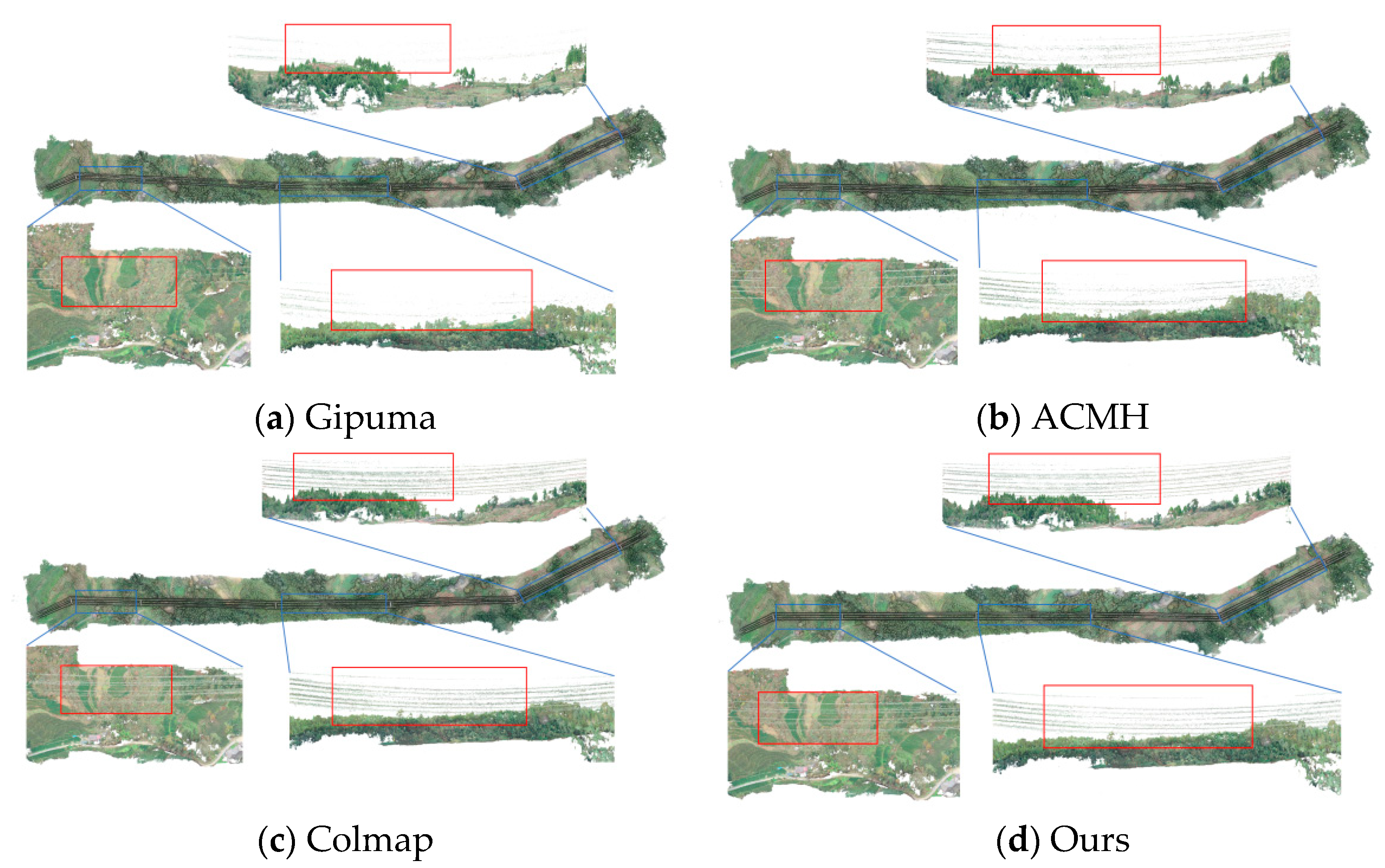
Secondly, this paper focuses on the comparative analysis of the reconstructed point clouds of power lines in the UAV images of the three test sites with the four different methods, as shown in Figure 7, Figure 8, and Figure 9, respectively. In test site 1, three spans’ point clouds of power lines are selected for visual comparison. From Figure 7, it can be seen that the power lines reconstruction result by Gipuma is the worst, and only a few power lines can be reconstructed in each bundled conductor. The ACMH can reconstruct the point clouds of power lines on both sides of the spans, but the point clouds in the middle of the spans are sparse and incomplete. Colmap and the proposed method can reconstruct more complete point clouds in each span, and the results of power lines are significantly better than those reconstructed by Gipuma and ACMH.
The two sides of test side 2 are hillsides, while the middle part is low, with a large height difference between both sides. Figure 8 is the results of the reconstructed power lines with different methods. From Figure 8, it can be seen that Gipuma can only reconstruct a few of the power lines on both sides of the span; while the ACMH can reconstruct relatively more complete point clouds of power lines than Gipuma, but in the middle region, parts of power line cannot be reconstructed; Colmap and the proposed method reconstruct power lines more completely than ACMH and Gipuma.
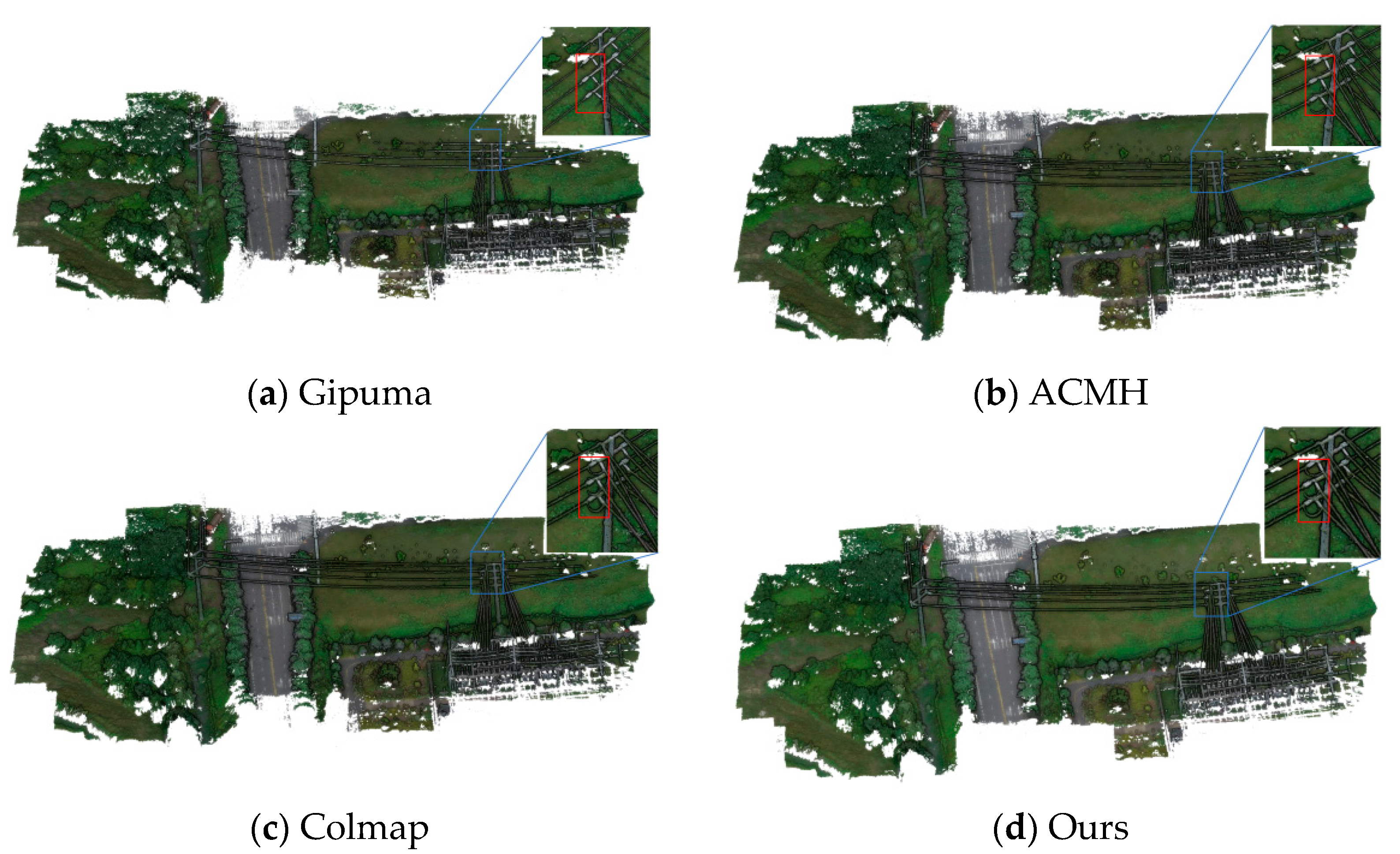
The terrain in test site 3 is relatively flat, including part of the transformer substation and roads. Figure 9 shows the comparison of the reconstructed power lines with different methods in test site 3. It can be seen that the Gipuma can only reconstruct part of the power lines, and there are many breaks at the uppermost power lines; ACMH, Colmap, and the proposed method can reconstruct power lines more completely than Gipuma. In addition, from the reconstructed jumper lines marked as blue rectangles in Figure 9, it can be seen that Gipuma failed to reconstruct the jumper lines; while ACMH can only reconstruct part of the jumper lines. Similarly, Colmap and the proposed method can reconstruct jumper lines more completely than Gipuma and ACMH.
Since the rectangle closed-loop trajectory is applied for UAV image collection, the intersection angle between adjacent images on the same side is small. If the images on the same side are selected for dense matching, the depth error of power lines would be augmented, which would be regarded as noise and removed in depth-map fusion. Therefore, the pixelwise visible image selection is extremely important for power line reconstruction with the rectangle closed-loop trajectory. In addition, because the power lines are suspended and the background in the image with different perspectives is different, the matching cost function directly affects the reconstruction result of power lines. The “top-k-winner-take-all” strategy is applied in Gipuma without robust pixelwise view selection, and the matching costs are the weight combinations of the color and gradient difference, which lead to poor performance on the reconstruction of power lines. Unlike Gipuma, the weighted bilateral NCC matching cost function is adopted in ACMH, Colmap, and the proposed method. Therefore, the main factors that affect the completeness of power lines are the view selection and the propagation mode. ACMH performs poorly in the completeness of power line reconstruction in test site 1 because it only uses pixels with the smallest matching cost in the fixed neighbor positions to select the visible image without taking into account the influence of the intersection angle. In addition, these pixels with sorted smallest matching costs are used to propagate the plane parameters. However, the matching cost of power lines is usually greater than that of the pixels of the ground. In this case, the pixels selected to propagate their plane parameters are located in the background of power lines, which leads to the low efficiency of propagation and the convergence speed of power lines is very slow in limited iterations. The structures of UAV images in test site 2 and test site 3 are stable, the propagation modes become the main factor that affects the completeness of reconstructed power lines. Due to the large terrain undulations and the large height difference between the terrain and power lines in test site 2, ACMH updates the depth and normal of power lines through the neighbor pixels with the smallest matching cost, which has poor propagation efficiency. The sequence propagation is adopted in Colmap, and the propagation direction in each iteration is changed to realize the depth and normal updating with the four neighbor pixels, which has high effectiveness for power line reconstruction. Random red-black propagation is applied in the proposed method, and the depth and normal are updated through the neighbor pixels with the most similar color, which can also ensure the effectiveness of the propagation for power lines. Compared with the results of Colmap, the proposed method has little difference from Colmap in the completeness of the reconstructed power lines.
3.2. Analysis of the Performance of Efficiency
In this experiment, the three datasets of the UAV images in the high-voltage power transmission line are selected to analyze the runtime performance. All the parameters are maintained the same as those in Section 3.1 and all the methods are run on the same platform. Figure 10 is a comparison chart of the total runtime of dense matching and depth map fusion with the four methods, and Table 2 lists the detailed runtime with the three high-voltage power transmission line datasets. Through comparative analysis, it can be seen that Colmap has the slowest runtime due to the sequence propagation, while Gipuma, ACMH, and the proposed method use diffusion-like propagation, which is more efficient and convenient for GPU parallel processing. However, bisection refinement is employed in Gipuma, which is time-consuming to generate more hypotheses to verify. ACMH directly accesses the color values from the texture memory in the GPU for matching cost computation, which does not make full use of the advantage of the shared memory technique of GPU. This paper fully combines the advantages of the above methods and adopts the random red-black checkerboard propagation and shared memory technique in GPU to improve efficiency. Moreover, two strategies for reducing the number of matching cost computations are adopted in the proposed method. Therefore, the runtime of the proposed method of PatchMatch is about 3–5 times faster than Colmap. With regards to depth-map fusion, it can be found that Colmap is the slowest, and the runtime is about 1/3 of the dense matching. ACMH and the proposed depth map fusion methods are more efficient than Colmap. The total runtime of the PatchMatch and depth-map fusion of the proposed method is about 4–7 times faster than Colmap.
4. Discussion
In this section, the analysis of the precision with the proposed method is discussed. The Strecha dataset and Vaihigen dataset are applied to verify the precision of the proposed method. The two benchmark datasets both provide the parameters of image orientations, the intrinsic parameters of the camera, and the ground truth mesh or point cloud. The accuracy, completeness, and score [43] are adopted for precision analysis.
In the experiment with the Strecha dataset, the image size is set 1563 × 1024 pixels and the maximum number of views selected for PatchMatch is set 10. In this experiment with the Vaihigen dataset, the image size is set 3889 × 7000 pixels, and the maximum number of views selected for PatchMatch is set 5. The remaining parameters are consistent with the experiment of the UAV images in the high-voltage power transmission line.
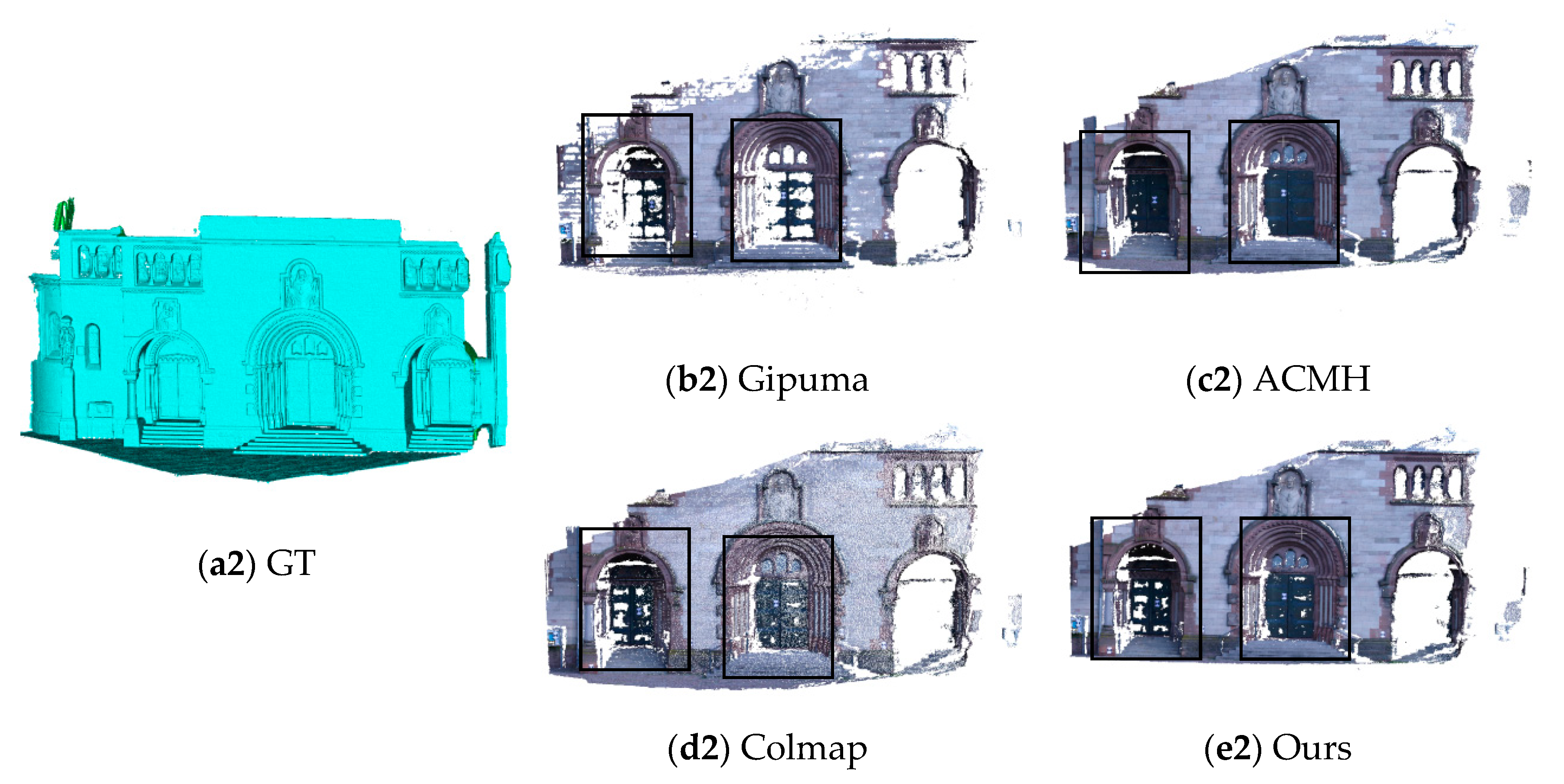
Figure 11 shows the comparison of reconstructed results of different methods in the Fountain and Herzjesu datasets. It can be seen that ACMH can match more point clouds on both sides of the Fountain dataset and at the gates of the Herzjesu dataset. This is mainly because there are coplanar areas in the two datasets, and the adaptive red-black checkerboard propagation adopted in ACMH can propagate the depth and normal in a larger range, which is more efficient in the coplanar areas and can improve the completeness in the low-textured areas. Gipuma performs worse than other methods in these two datasets. The proposed method can match slightly more point clouds on both sides of the Fountain dataset than Colmap, indicating that the random red-black checkerboard propagation adopted in the proposed method is better than the sequence propagation of Colmap in the coplanar regions but still worse than the adaptive red-black propagation of ACMH.
In addition, this paper quantitatively analyses the precision of point clouds reconstructed by the four methods in the Strecha dataset, in which the accuracy, completeness, and score of point clouds are used. The vertexes of the meshes in the Fountain and Herzjesu datasets are used as ground truth point clouds for the precision analysis. Table 3 shows the accuracy, completeness, and score with the evaluation threshold of 2 cm and 10 cm in percentage. It can be seen that Gipuma achieves the highest accuracy of the two datasets with the 2 cm and 10 cm thresholds because the bisection refinement is applied in Gipuma to obtain more accurate depth values. However, Gipuma performs worse in terms of completeness and score. ACMH has the highest completeness and score in the Fountain dataset with 2 cm and 10 cm, and in the Herzjesu dataset with a 2 cm threshold, indicating that ACMH has advantages in the coplanar regions. The score of the proposed method is higher than that of Colmap, which verifies that the random red-black propagation can improve the propagation efficiency.
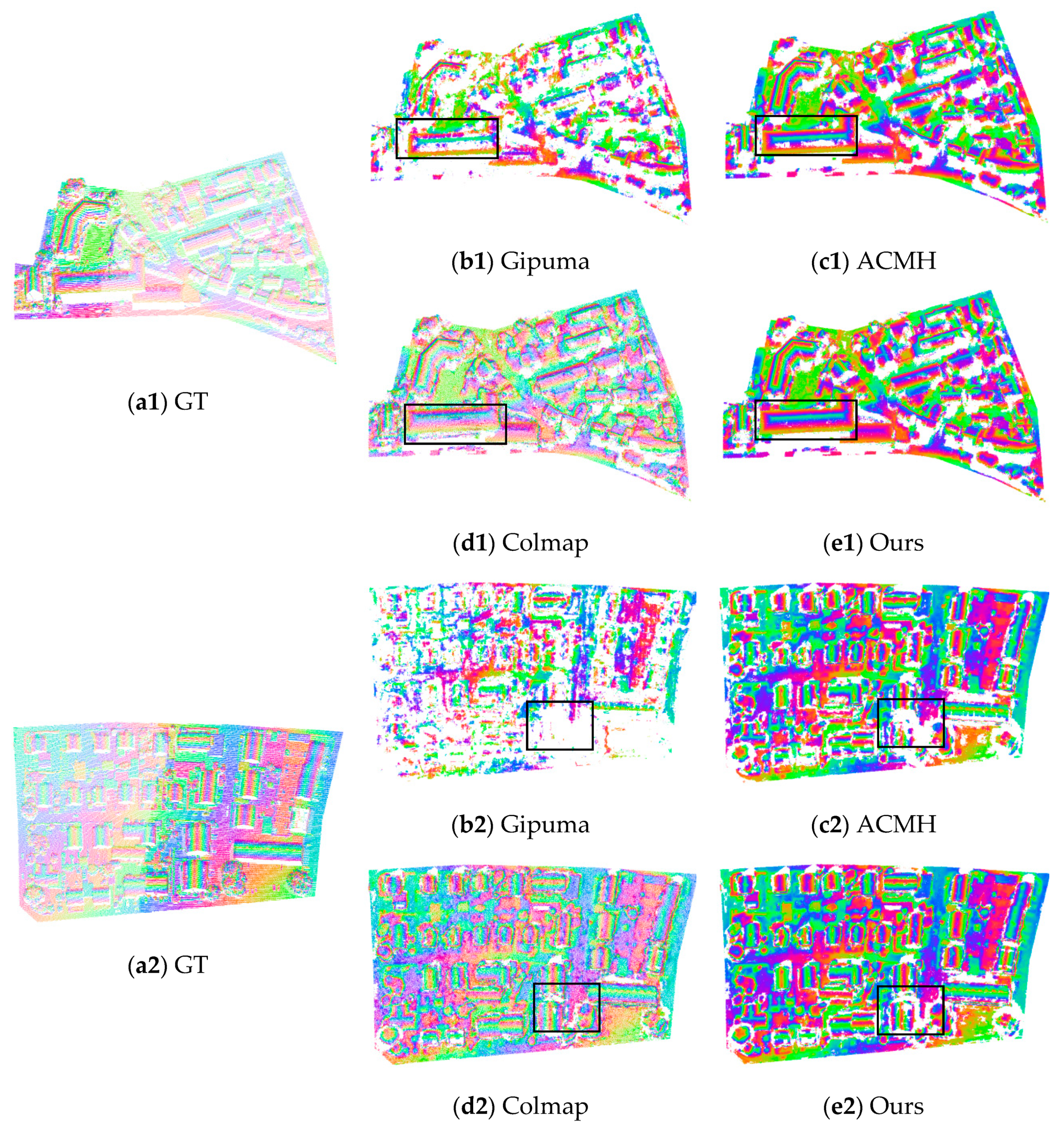
Figure 12 shows the ground truth point clouds and the results of reconstructed point clouds in test site 1 and test site 3 of the Vaihigen with different methods. It can be seen that Gipuma has the worst completeness with a large number of holes in both test sites. ACMH, Colmap, and the proposed method all have poor performance in the road regions because the roads are weakly textured with fewer color changes and they are difficult to match with bilateral weighted NCC. It can also be found that the completeness of ACMH in test site 1 marked with a black rectangle is worse than Colmap and the proposed method. The reconstructed point clouds of Colmap in test site 3 marked with a black rectangle are better than the other three methods.
Similarly, the accuracy, completeness, and score are used for quantitative evaluation with the thresholds of 0.2 m and 0.5 m, as shown in Table 4. It can be seen that Gipuma has the highest accuracy in test site 1 with the evaluation threshold of 0.5 m, but has the lowest score in both test sites similar to the Strecha dataset. ACMH has the highest accuracy and score in both test sites with the evaluation threshold of 0.2 m; the proposed method achieves the highest score in both test sites with an evaluation threshold of 0.5 m. It can also be found that the scores in both test sites of the Vaihigen dataset of the proposed method are better than Colmap.
5. Conclusions
An improved fast PatchMatch method for the UAV images of high-voltage power transmission lines is proposed based on Colmap, which can greatly improve efficiency while ensuring the completeness of the reconstruction of power lines. This paper employs the following three aspects to improve the efficiency of Colmap. Firstly, a new random red-black checkerboard propagation is proposed. By randomly sampling the neighbor pixels with different color patterns, the pixels with the most similar color to the current pixel are selected to propagate the plane parameters, which is more conducive to the reconstruction of power lines compared with the adaptive red-black propagation in ACMH. To combine the pixelwise view selection strategy in Colmap with the efficient random red-black checkerboard propagation, the updating schedule of hidden variables adopted in Colmap is improved. Secondly, strategies for reducing the number of matching cost computations are adopted. The number of neighbor pixels for the plane parameters propagation is reduced with the increasing of iteration number; the number of combinations with the depth and normal hypotheses is reduced in the plane refinement procedure according to the matching cost. Finally, an efficient depth map fusion is implemented in the GPU, which uses the weighted function based on reprojection error to fuse depth values. Through these strategies, the efficiencies of dense matching and depth-map fusion are greatly improved.
The experiments with UAV images of high-voltage power transmission lines from three test sites show that the proposed method can reconstruct more complete point clouds of power lines than Gipuma and ACMH, and the reconstructed power lines are more similar to Colmap. With the analysis of runtime performance, the proposed method achieves 4–7 times faster than that of Colmap. Experiments of the precision analysis with two benchmark datasets, Strecha and Vaihigen, demonstrate that the score of the proposed method is higher than Colmap. Comprehensive experiments indicate that the proposed method has promising application for high-voltage power transmission lines.
Author Contributions
Conceptualization, W.J. and W.H.; methodology, W.H. and W.J.; software, W.H. and S.J.; validation, W.J., S.J. and W.H.; formal analysis, W.J. and S.J.; investigation, W.H.; resources, W.J.; data curation, S.J.; writing—original draft preparation, W.H.; writing—review and editing, W.J., S.J. and S.H.; visualization, W.H. and S.H.; supervision, W.J.; project administration, W.J.; funding acquisition, W.J. and S.J. All authors have read and agreed to the published version of the manuscript.
Funding
This research was supported by funds from the “National Natural Science Foundation of China” (grant No. 42001413) and the “China High-Resolution Earth Observation System Based Demonstration System of Remote Sensing Application for Urban Refined Management (Phase II)” (grant No. 06-Y30F04-9001-20/22).
Institutional Review Board Statement
Not applicable.
Informed Consent Statement
Not applicable.
Data Availability Statement
Data available in a publicly accessible repository that does not issue DOIs Publicly available datasets were analyzed in this study. Strecha and Vaihigen Datasets can be found here: [https://documents.epfl.ch/groups/c/cv/cvlab-unit/www/data/multiview/denseMVS.html, accessed on 13 October 2021; https://www2.isprs.org/commissions/comm2/wg4/benchmark/2d-sem-label-vaihingen/, accessed on 13 October 2021]. The three test site datasets of UAV images in high transmission lines are available on request from the corresponding author.
Acknowledgments
The authors thank the researchers of Colmap, Gipuma and ACMH for providing the codes. The authors would like to express their gratitude to the editors and the anonymous reviewers for their professional and help comments, which are of great help to the improvement of this study.
Conflicts of Interest
The authors declare no conflict of interest.
References
- Jiang, S.; Jiang, W.; Huang, W.; Yang, L. UAV-Based Oblique Photogrammetry for Outdoor Data Acquisition and Offsite Visual Inspection of Transmission Line. Remote Sens. 2017, 9, 278. [Google Scholar] [CrossRef] [Green Version]
- Agarwal, S.; Furukawa, Y.; Snavely, N.; Simon, I.; Curless, B.; Seitz, S.; Szeliski, R. Building Rome in a Day. Commun. ACM. 2011, 54, 105–112. [Google Scholar] [CrossRef]
- Schönberger, J.L.; Frahm, J.-M. Structure-from-Motion Revisited. In Proceedings of the IEEE Conference on Computer Vision and Pattern Recognition (CVPR), Las Vegas, NV, USA, 27–30 June 2016; 2016; pp. 4104–4113. [Google Scholar] [CrossRef]
- Jiang, S.; Jiang, W. Efficient SfM for Oblique UAV Images: From Match Pair Selection to Geometrical Verification. Remote Sens. 2018, 10, 1246. [Google Scholar] [CrossRef] [Green Version]
- Jiang, S.; Jiang, W. Efficient Structure from Motion for Oblique UAV Images Based on Maximal Spanning Tree Expansion. ISPRS J. Photogramm. Remote Sens. 2017, 132, 140–161. [Google Scholar] [CrossRef]
- Jiang, S.; Jiang, C.; Jiang, W. Efficient Structure from Motion for Large-scale UAV Images: A Review and a Comparison of SfM Tools. ISPRS J. Photogramm. Remote Sens. 2020, 167, 230–251. [Google Scholar] [CrossRef]
- Stentoumis, C.; Grammatikopoulos, L.; Kalisperakis, I.; Karras, G. On Accurate Dense Stereo-matching Using a Local Adaptive Multi-cost Approach. ISPRS J. Photogramm. Remote Sens. 2014, 91, 29–49. [Google Scholar] [CrossRef]
- Furukawa, Y.; Hernandez, C. Multi-View Stereo: A Tutorial. Found. Trends Comput. Graph. Vis. 2015, 9, 1–148. [Google Scholar] [CrossRef] [Green Version]
- Chen, C.; Seff, A.; Kornhauser, A.; Xiao, J. Deepdriving: Learning Affordance for Direct Perception in Autonomous Driving. In Proceedings of the IEEE International Conference on Computer Vision (ICCV), Las Condes, Chile, 11–18 December 2015; pp. 2722–2730. [Google Scholar] [CrossRef] [Green Version]
- Haque, A.U.; Nejadpak, A. Obstacle Avoidance Using Stereo Camera. arXiv 2017, arXiv:1705.04114. [Google Scholar]
- Günen, M.; Beşdok, P.; Besdok, E. Use of Potree and Cesium Platforms for Presentation of Point Clouds. In Proceedings of the International Symposium on Innovative Approaches in Scientific Studies, Antalya, Turkey, 19 April 2018; p. 58. [Google Scholar]
- Rhee, S.; Kim, T. Automated DSM Extraction from UAV Images and Performance Analysis. In Proceedings of the International Conference on Unmanned Aerial Vehicles in Geomatics, Toronto, ON, Canada, 30 August–2 September 2015; pp. 351–354. [Google Scholar] [CrossRef] [Green Version]
- Zhang, Y.; Yuan, X.; Li, W.; Chen, S. Automatic Power Line Inspection Using UAV Images. Remote Sens. 2017, 9, 824. [Google Scholar] [CrossRef] [Green Version]
- Seitz, S.M.; Curless, B.; Diebel, J.; Scharstein, D.; Szeliski, R. A Comparison and Evaluation of Multi-View Stereo Reconstruction Algorithms. In Proceedings of the 2006 IEEE Computer Society Conference on Computer Vision and Pattern Recognition, New York, NY, USA , 17–22 June 2006; 2006; pp. 519–528. [Google Scholar] [CrossRef]
- Vu, H.H.; Keriven, R.; Labatut, P.; Pons, J.P. Towards High-resolution Large-scale Multi-view Stereo. In Proceedings of the IEEE Conference on Computer Vision and Pattern Recognition, Miami, FL, USA, 20–25 June 2009; pp. 1430–1437. [Google Scholar] [CrossRef] [Green Version]
- Cremers, D.; Kolev, K. Multiview Stereo and Silhouette Consistency via Convex Functionals over Convex Domains. IEEE Trans. Pattern Anal. Mach. Intell. 2011, 33, 1161–1174. [Google Scholar] [CrossRef] [Green Version]
- Sinha, S.N.; Mordohai, P.; Pollefeys, M. Multi-View Stereo via Graph Cuts on the Dual of an Adaptive Tetrahedral Mesh. In Proceedings of the IEEE International Conference on Computer Vision, Rio de Janeiro, Brazil, 14–21 October 2007; pp. 1–8. [Google Scholar] [CrossRef]
- Furukawa, Y.; Ponce, J. Accurate, Dense, and Robust Multiview Stereopsis. IEEE Trans. Pattern Anal. Mach. Intell. 2010, 32, 1362–1376. [Google Scholar] [CrossRef]
- Goesele, M.; Snavely, N.; Curless, B.; Hoppe, H.; Seitz, S.M. Multi-View Stereo for Community Photo Collections. In Proceedings of the IEEE 11th International Conference on Computer Vision, Rio de Janeiro, Brazil, 14–21 October 2007; pp. 1–8. [Google Scholar] [CrossRef]
- Galliani, S.; Lasinger, K.; Schindler, K. Massively Parallel Multiview Stereopsis by Surface Normal Diffusion. In Proceedings of the IEEE International Conference on Computer Vision, Las Condes, Chile, 11–18 December 2015; pp. 873–881. [Google Scholar] [CrossRef]
- Schönberger, J.L.; Zheng, E.; Pollefeys, M.; Frahm, J.M. Pixelwise View Selection for Unstructured Multi-View Stereo. In Proceedings of the European Conference on Computer Vision; Springer: Cham, Switzerland, 2016; pp. 501–518. [Google Scholar] [CrossRef]
- Xu, Q.; Tao, W. Multi-Scale Geometric Consistency Guided Multi-View Stereo. In Proceedings of the IEEE/CVF Conference on Computer Vision and Pattern Recognition, Long Beach, CA, USA, 15–21 June 2019; pp. 5483–5492. [Google Scholar] [CrossRef] [Green Version]
- Hirschmüller, H. Stereo Processing by Semiglobal Matching and Mutual Information. IEEE Trans. Pattern Anal. Mach. Intell. 2008, 30, 328–341. [Google Scholar] [CrossRef]
- Barnes, C.; Shechtman, E.; Finkelstein, A.; Dan, B.G. PatchMatch: A Randomized Correspondence Algorithm for Structural Image Editing. ACM Trans. Graph. 2009, 28, 24. [Google Scholar] [CrossRef]
- Barnes, C.; Shechtman, E.; Dan, B.G.; Finkelstein, A. The Generalized PatchMatch Correspondence Algorithm. In Proceedings of the European Conference on Computer Vision, Heraklion, Greece, 5–11 September 2010; pp. 29–43. [Google Scholar] [CrossRef]
- Liao, J.; Fu, Y.; Yan, Q.; Xiao, C. Pyramid Multi-View Stereo with Local Consistency. Comput. Graph. Forum. 2019, 38, 335–346. [Google Scholar] [CrossRef]
- Bleyer, M.; Rhemann, C.; Rother, C. PatchMatch Stereo—Stereo Matching with Slanted Support Windows. In Proceedings of the British Machine Vision Conference, Dundee, UK, 29 August–2 September 2011; pp. 1–11. [Google Scholar]
- Heise, P.; Klose, S.; Jensen, B.; Knoll, A. PM-Huber: PatchMatch with Huber Regularization for Stereo Matching. In Proceedings of the IEEE International Conference on Computer Vision, Columbus, OH, USA, 23–28 June 2014; pp. 2360–2367. [Google Scholar] [CrossRef] [Green Version]
- Besse, F.; Rother, C.; Fitzgibbon, A.; Kautz, J. PMBP: PatchMatch Belief Propagation for Correspondence Field Estimation. Int. J. Comput. Vis. 2014, 110, 2–13. [Google Scholar] [CrossRef]
- Yu, L.; Min, D.; Brown, M.S.; Do, M.N.; Lu, J. SPM-BP: Sped-Up PatchMatch Belief Propagation for Continuous MRFs. In Proceedings of the IEEE International Conference on Computer Vision, Santiago, Chile, 7–13 December 2015; pp. 4006–4014. [Google Scholar] [CrossRef]
- Xu, S.; Zhang, F.; He, X.; Shen, X.; Zhang, X. PM-PM: PatchMatch with Potts Model for Object Segmentation and Stereo Matching. IEEE Trans. Image Process. 2015, 24, 2182–2196. [Google Scholar] [CrossRef]
- Lu, J.; Yu, L.; Yang, H.; Min, D.; Eng, W.; Do, M.N. PatchMatch Filter: Edge-Aware Filtering Meets Randomized Search for Visual Correspondence. IEEE Trans. Pattern Anal. Mach. Intell. 2017, 39, 1866–1879. [Google Scholar] [CrossRef]
- Tian, M.; Yang, B.; Chen, C.; Huang, R.; Huo, L. HPM-TDP: An efficient hierarchical PatchMatch depth estimation approach using tree dynamic programming. ISPRS J. Photogramm. Remote Sens. 2019, 155, 37–57. [Google Scholar] [CrossRef]
- Shen, S. Accurate Multiple View 3D Reconstruction Using Patch-Based Stereo for Large-Scale Scenes. IEEE Trans. Image Process. 2013, 22, 1901–1914. [Google Scholar] [CrossRef]
- Zheng, E.; Dunn, E.; Jojic, V.; Frahm, J.M. PatchMatch Based Joint View Selection and Depthmap Estimation. In Proceedings of the IEEE Conference on Computer Vision and Pattern Recognition, Columbus, OH, USA, 23–28 June 2014; pp. 1510–1517. [Google Scholar] [CrossRef]
- Romanoni, A.; Matteucci, M. TAPA-MVS: Textureless-Aware PAtchMatch Multi-View Stereo. In Proceedings of the 2019 IEEE/CVF International Conference on Computer Vision, Seoul, Korea, 27 October–2 November 2019; pp. 10413–10422. [Google Scholar] [CrossRef] [Green Version]
- Xu, Q.; Tao, W. Planar Prior Assisted PatchMatch Multi-View Stereo. In Proceedings of the AAAI Conference on Artificial Intelligence, New York, NY, USA, 7–12 February 2020; pp. 12516–12523. [Google Scholar] [CrossRef]
- Hou, Y.; Peng, J.; Hu, Z.; Tao, P.; Shan, J. Planarity Constrained Multi-view Depth Map Reconstruction for Urban Scenes. ISPRS J. Photogramm. Remote Sens. 2018, 139, 133–145. [Google Scholar] [CrossRef]
- Strecha, C.; Hansen, W.V.; Gool, L.V.; Fua, P.; Thoennessen, U. On Benchmarking Camera Calibration and Multi-View Stereo for High Resolution Imagery. In Proceedings of the IEEE Conference on Computer Vision and Pattern Recognition, Anchorage, AK, USA, 23-28 June 2008; pp. 1–8. [Google Scholar] [CrossRef]
- Cramer, M. The DGPF-test on digital airborne camera evaluation overview and test design. Photogramm. Fernerkund. Geoinf. 2010, 73–82. [Google Scholar] [CrossRef]
- Hane, C.; Zach, C.; Cohen, A.; Angst, R.; Pollefeys, M. Joint 3D Scene Reconstruction and Class Segmentation. In Proceedings of the IEEE Conference on Computer Vision and Pattern Recognition, Portland, OR, USA, 23–28 June 2013; pp. 97–104. [Google Scholar] [CrossRef]
- Curless, B.; Levoy, M. A Volumetric Method for Building Complex Models from Range Images. In Proceedings of the 23rd Annual Conference on Computer Graphics and Interactive Techniques, New Orleans, LA, USA, 4–9 August 1996; pp. 303–312. [Google Scholar]
- Knapitsch, A.; Park, J.; Zhou, Q.-Y.; Koltun, V. Tanks and Temples: Benchmarking Large-scale Scene Reconstruction. ACM Trans. Graph. 2017, 36, 1–13. [Google Scholar] [CrossRef]
Figure 1.
UAV images of the three test sites. (a–c) are the rectangle dataset in test site 1, S-shaped dataset in test site 2, and traditional multiple trajectories dataset in test site 3, respectively.
Figure 1.
UAV images of the three test sites. (a–c) are the rectangle dataset in test site 1, S-shaped dataset in test site 2, and traditional multiple trajectories dataset in test site 3, respectively.

Figure 2.
Two test sites in the Vaihigen dataset: (a,b) are test site 1 and test site 3, respectively.
Figure 2.
Two test sites in the Vaihigen dataset: (a,b) are test site 1 and test site 3, respectively.

Figure 3.
The visibility state variable updating schedule adopted in Colmap [35].
Figure 3.
The visibility state variable updating schedule adopted in Colmap [35].

Figure 4.
Comparison of the depth maps with three different view selection and propagation strategies. (a1,b1) are the results of the “top-k-winners-take-all” strategy with symmetric red-black propagation; (a2,b2) are the results of Colmap with sequence propagation; (a3,b3) are the results of the proposed strategy with random red-black propagation.

Figure 5.
The relationship of accuracy and iteration number. (a) is the percentage of pixels with absolute errors below 2 cm and 10 cm. (b–e) are the depth maps with iterations of 1, 3, 5, and 7.
Figure 5.
The relationship of accuracy and iteration number. (a) is the percentage of pixels with absolute errors below 2 cm and 10 cm. (b–e) are the depth maps with iterations of 1, 3, 5, and 7.

Figure 6.
Depth maps comparison with different methods. (a–d) are generated by Gipuma, ACMH, Colmap, and the proposed method, respectively.
Figure 6.
Depth maps comparison with different methods. (a–d) are generated by Gipuma, ACMH, Colmap, and the proposed method, respectively.

Figure 7.
The comparison of reconstructed point clouds of power lines in test site 1. (a–d) are generated by Gipuma, ACMH, Colmap, and the proposed method, respectively.
Figure 7.
The comparison of reconstructed point clouds of power lines in test site 1. (a–d) are generated by Gipuma, ACMH, Colmap, and the proposed method, respectively.

Figure 8.
The comparison of reconstructed point clouds of power lines in test site 2. (a–d) are generated by Gipuma, ACMH, Colmap, and the proposed method, respectively.
Figure 8.
The comparison of reconstructed point clouds of power lines in test site 2. (a–d) are generated by Gipuma, ACMH, Colmap, and the proposed method, respectively.

Figure 9.
The comparison of reconstructed point clouds of power lines in test site 3. (a–d) are generated by Gipuma, ACMH, Colmap, and the proposed method, respectively.
Figure 9.
The comparison of reconstructed point clouds of power lines in test site 3. (a–d) are generated by Gipuma, ACMH, Colmap, and the proposed method, respectively.

Figure 10.
The comparison of total runtimes of dense matching and depth map fusion with different methods.
Figure 10.
The comparison of total runtimes of dense matching and depth map fusion with different methods.

Figure 11.
The comparison of reconstructed point clouds with the Strecha dataset. (a1,a2) are the ground truth meshes of the Fountain and Herzjesu datasets, respectively. (b1–e1) and (b2–e2) are generated by Gipuma, ACMH, Colmap, and the proposed method with the Fountain and Herzjesu datasets, respectively.


Figure 12.
The comparison of reconstructed point clouds with test site 1 and test site 3 in the Vaihigen dataset. (a1,a2) are the ground truth point clouds of test site 1 and test site 3, respectively. (b1–e1) and (b2–e2) are generated by Gipuma, ACMH, Colmap, and the proposed method with test site 1 and test site 3, respectively.


Table 1.
Details of the three test sites.
| Item Name | Test Site 1 | Test Site 2 | Test Site 3 |
|---|---|---|---|
| Flight mode | rectangle | S-shaped | multiple trajectories |
| Flight height (m) | 160 | 80 | 65 |
| Voltage (kV) | 500 | 220 | 110 |
| Bundled conductors | 4-bundled | 2-bundled | 1-bundled |
| Type of UAV | DJI Phantom 4 RTK | ||
| Image size | 5472 × 3078 | 4864 × 3648 | 5472 × 3078 |
| Image number | 222 | 191 | 103 |
| GSD (cm) | 4.70 | 2.72 | 1.75 |
Table 2.
Details of the runtime of dense matching and depth map fusion with different methods for the three datasets in the high-voltage power transmission line.
Table 2.
Details of the runtime of dense matching and depth map fusion with different methods for the three datasets in the high-voltage power transmission line.
| Methods | Test Site 1/(Min) | Test Site 2/(Min) | Test Site 3/(Min) | |
|---|---|---|---|---|
| Gipuma | PatchMatch | 139.04 | 52.74 | 34.12 |
| Depth fusion | 7.75 | 4.88 | 2.38 | |
| Total | 146.79 | 57.62 | 36.50 | |
| ACMH | PatchMatch | 92.39 | 31.82 | 19.56 |
| Depth fusion | 7.75 | 4.88 | 2.38 | |
| Total | 100.14 | 36.70 | 21.94 | |
| Colmap | PatchMatch | 201.03 | 117.28 | 75.04 |
| Depth fusion | 78.54 | 58.62 | 41.07 | |
| Total | 279.57 | 175.90 | 116.11 | |
| Ours | PatchMatch | 58.55 | 22.62 | 14.09 |
| Depth fusion | 7.07 | 3.86 | 2.35 | |
| Total | 65.62 | 26.48 | 16.44 | |
Table 3.
The precision comparison of point clouds with different methods in the Strecha dataset. The accuracy (A), completeness (C), and score (in %) are evaluated with 2 cm and 10 cm thresholds.
Table 3.
The precision comparison of point clouds with different methods in the Strecha dataset. The accuracy (A), completeness (C), and score (in %) are evaluated with 2 cm and 10 cm thresholds.
| Datasets | Methods | 2 cm/(%) | 10 cm/(%) | ||||
|---|---|---|---|---|---|---|---|
| A | C | A | C | ||||
| Fountain | Gipuma | 84.47 | 41.39 | 55.56 | 97.54 | 54.33 | 69.79 |
| ACMH | 74.83 | 48.95 | 59.19 | 95.83 | 60.32 | 74.04 | |
| Colmap | 75.08 | 44.72 | 56.05 | 95.18 | 58.71 | 72.62 | |
| Ours | 74.61 | 47.20 | 57.82 | 95.26 | 59.44 | 73.20 | |
| Herzjesu | Gipuma | 78.42 | 29.53 | 42.90 | 96.43 | 47.78 | 63.90 |
| ACMH | 74.08 | 39.51 | 51.53 | 94.52 | 54.75 | 69.34 | |
| Colmap | 67.28 | 32.84 | 44.13 | 92.26 | 55.20 | 69.07 | |
| Ours | 73.16 | 37.78 | 49.83 | 94.28 | 54.73 | 69.25 | |
Table 4.
The precision comparison of point clouds with different methods in test site 1 and test site 3 of the Vaihigen dataset. The accuracy (A), completeness (C), and score (in %) are evaluated with 0.2 m and 0.5 m thresholds.
Table 4.
The precision comparison of point clouds with different methods in test site 1 and test site 3 of the Vaihigen dataset. The accuracy (A), completeness (C), and score (in %) are evaluated with 0.2 m and 0.5 m thresholds.
| Datasets | Methods | 0.2 m (%) | 0.5 m(%) | ||||
|---|---|---|---|---|---|---|---|
| A | C | A | C | ||||
| Test site 1 | Gipuma | 37.11 | 23.35 | 28.66 | 71.68 | 50.32 | 59.13 |
| ACMH | 39.91 | 41.10 | 40.50 | 68.35 | 65.23 | 66.76 | |
| Colmap | 32.64 | 26.59 | 29.31 | 55.80 | 66.32 | 60.61 | |
| Ours | 38.62 | 42.11 | 40.29 | 66.29 | 67.58 | 66.93 | |
| Test site 3 | Gipuma | 36.47 | 16.27 | 22.50 | 73.85 | 41.43 | 53.08 |
| ACMH | 40.92 | 38.88 | 39.87 | 74.93 | 65.99 | 70.17 | |
| Colmap | 36.26 | 26.92 | 30.90 | 64.41 | 71.18 | 67.63 | |
| Ours | 37.04 | 37.40 | 37.22 | 72.08 | 69.78 | 70.91 | |
Publisher’s Note: MDPI stays neutral with regard to jurisdictional claims in published maps and institutional affiliations. |
© 2021 by the authors. Licensee MDPI, Basel, Switzerland. This article is an open access article distributed under the terms and conditions of the Creative Commons Attribution (CC BY) license (https://creativecommons.org/licenses/by/4.0/).
Share and Cite
MDPI and ACS Style
Huang, W.; Jiang, S.; He, S.; Jiang, W. Accelerated Multi-View Stereo for 3D Reconstruction of Transmission Corridor with Fine-Scale Power Line. Remote Sens. 2021, 13, 4097. https://doi.org/10.3390/rs13204097
AMA Style
Huang W, Jiang S, He S, Jiang W. Accelerated Multi-View Stereo for 3D Reconstruction of Transmission Corridor with Fine-Scale Power Line. Remote Sensing. 2021; 13(20):4097. https://doi.org/10.3390/rs13204097
Chicago/Turabian StyleHuang, Wei, San Jiang, Sheng He, and Wanshou Jiang. 2021. "Accelerated Multi-View Stereo for 3D Reconstruction of Transmission Corridor with Fine-Scale Power Line" Remote Sensing 13, no. 20: 4097. https://doi.org/10.3390/rs13204097
Note that from the first issue of 2016, this journal uses article numbers instead of page numbers. See further details here.