Article

Camera Self-Calibration with GNSS Constrained Bundle Adjustment for Weakly Structured Long Corridor UAV Images

1
State Key Laboratory of Information Engineering in Surveying, Mapping and Remote Sensing, Wuhan University, 129 Luoyu Road, Wuhan 430079, China
2
School of Computer Science, China University of Geosciences, Wuhan 430074, China
3
Collaborative Innovation Center of Geospatial Technology, Wuhan University, 129 Luoyu Road, Wuhan 430079, China
*
Author to whom correspondence should be addressed.
Remote Sens. 2021, 13(21), 4222; https://doi.org/10.3390/rs13214222
Submission received: 14 September 2021 / Revised: 4 October 2021 / Accepted: 18 October 2021 / Published: 21 October 2021
(This article belongs to the Special Issue Techniques and Applications of UAV-Based Photogrammetric 3D Mapping)

Abstract

:
Camera self-calibration determines the precision and robustness of AT (aerial triangulation) for UAV (unmanned aerial vehicle) images. The UAV images collected from long transmission line corridors are critical configurations, which may lead to the “bowl effect” with camera self-calibration. To solve such problems, traditional methods rely on more than three GCPs (ground control points), while this study designs a new self-calibration method with only one GCP. First, existing camera distortion models are grouped into two categories, i.e., physical and mathematical models, and their mathematical formulas are exploited in detail. Second, within an incremental SfM (Structure from Motion) framework, a camera self-calibration method is designed, which combines the strategies for initializing camera distortion parameters and fusing high-precision GNSS (Global Navigation Satellite System) observations. The former is achieved by using an iterative optimization algorithm that progressively optimizes camera parameters; the latter is implemented through inequality constrained BA (bundle adjustment). Finally, by using four UAV datasets collected from two sites with two data acquisition modes, the proposed algorithm is comprehensively analyzed and verified, and the experimental results demonstrate that the proposed method can dramatically alleviate the “bowl effect” of self-calibration for weakly structured long corridor UAV images, and the horizontal and vertical accuracy can reach 0.04 m and 0.05 m, respectively, when using one GCP. In addition, compared with open-source and commercial software, the proposed method achieves competitive or better performance.

Graphical Abstract

1. Introduction

With the advantages of flexible data acquisition and ease of use, UAV has become one of the most important remote sensing platforms for the photogrammetry and remote sensing community [1]. The UAVs have the characteristics of small size, autonomous vertical take-off and landing with low site requirements, high flight safety performance, and the flexibility to adjust the direction of flight, making them widely used for the regular inspection of high-voltage transmission line corridors [2,3,4,5,6]. However, the UAV platforms are often equipped with consumer-grade, non-metric digital cameras, mainly due to the limitations of the platform’s load capacity. These cameras have non-ignored lens distortions when compared with metric sensors, which influences the robustness and precision of AT. The long corridor structure of UAV images is a critical configuration, and the reconstructed model would be bending with the inaccurately estimated distortion parameters. For example, Figure 1 illustrates the “bowl effect” of self-calibration with commercial software and open-source software for long corridor UAV images because of the failure in camera distortion parameter estimation. Thus, it is very critical to accurately estimate the distortion parameters of cameras for high-precision AT.
In photogrammetry and computer vision fields, the purpose of camera self-calibration is to solve the internal orientation parameters and camera lens distortion parameters, which affect the precision of 3D reconstruction. At present, the existing camera calibration methods can be categorized into two groups: pre-calibration and self-calibration. The pre-calibration method usually depends on either the indoor calibration board with fixed patterns [7,8] or the outer door large-scale 3D calibration test field [9]. However, this kind of method has many disadvantages applied in UAV image calibration. On the one hand, the indoor calibration errors of the calibration board with special patterns would be expanded with the increase of UAV flying height, and the focal length of the camera is usually set to be fixed depending on the flying height of UAVs, which is not suitable for indoor camera pre-calibration; on the other hand, although the outer door 3D calibration test field could improve the precision of camera calibration, it requires a lot of manpower and consumes time. Compared with the drawbacks of pre-calibration, the self-calibration process is simpler and more convenient without any known calibration targets.
With the above considerations, the relevant scholars have performed in-depth research on the camera self-calibration methods with different camera distortion models, including the physical model and mathematical model. Among the camera distortion models, the Brown model [10] and its improved model [11] are the most classical physical models. However, it is a challenge for camera self-calibration to occur in the critical configuration, due to the high correlation between the distortion parameters of the Brown model [12]. In the field of computer vision, the division model is another kind of physical model commonly used [13], which can fit simple camera distortion. Recently, many researchers have combined the division model with the fundamental matrix or the essential matrix to solve the camera distortion parameters by establishing polynomial equations [14,15,16,17]. However, it cannot fit complex camera distortion and is not suitable for UAV camera self-calibration. The physical camera model cannot describe the complex distortion precisely and may not work when the pattern of camera distortion is not apparent and the precise knowledge on distortion is unavailable. Based on this consideration, the mathematical model tries to use function approximation theory to accurately fit complex camera distortion, such as the quadratic orthogonal polynomial [18] and quartic orthogonal polynomial model [19]. Tang et al. [20,21] proposed the orthogonal polynomial models based on Legendre and Fourier polynomials and applied the models in an aerial camera for self-calibration. Subsequently, Babapour et al. [22] presented the Chebyshev–Fourier and Jacobi–Fourier camera models, which significantly improved the horizontal and elevation accuracy of aerial images. However, few studies have applied the Legendre- and Fourier-based distortion models to camera self-calibration for long corridor UAV images. This is the first key research content of this paper.
For the camera self-calibration with a long corridor structure, the related research can be divided into three categories: the research on the theoretic analysis [23,24], the research on the strategies of self-calibration [25,26], and the accuracy verification with such structures [27,28,29,30,31,32]. Wu et al. [23] analyzed the motion field of images with radial distortion and proved the ambiguous reconstruction with the “bowl effect” of camera self-calibration under weak structures and configuration through mathematical theory. Zhou et al. [24] discussed the impact of the focal length parameter estimation of camera self-calibration with a flat, corridor configuration. The research on the theoretic analysis of camera self-calibration with a long corridor structure has focused on investigating the causes and influencing factors, but has not presented any solutions to solve the problems. For the long corridor structure, Tournadre et al. [25] presented a 7th-order polynomial combined with radial camera distortion model (F15P7) and verified the accuracy of the orientations with a weak configuration using ground control points (GCP). Although this method can alleviate the “bowl effect”, it relied on more than three GCPs for absolute image orientation. Polic et al. [26] proposed an uncertainty-based camera model selection method to reduce the “bowl effect”, but this method did not consider the newest mathematical-based distortion models and high-precision GNSS observations. Griffiths et al. [27] analyzed the accuracy of 3D reconstruction from long corridor structure UAV images in detail, and experiments show that the more complex distortion model can improve the accuracy of camera self-calibration. The related works of [28,29,30,31,32] are mainly focused on accessing the accuracy of the DSM (Digital Surface Model), DTM (Digital Terrain Model), the influence of the distribution of GCPs, and on giving suggestions for data collection without improvement of the strategies for camera self-calibration. Compared to the existing literature about self-calibration with a long corridor structure, the proposed paper extends the scope of research on camera distortion models and investigates the accuracy of the recently proposed orthogonal polynomial model with the strategies for camera parameter initialization and high-precision GNSS fusion in a long corridor structure.
For the traditional aerial photogrammetry in surveying and mapping, the UAV platform generally collects image data with the regular region and often has multiple parallel and overlapping stable structures. However, in the application of UAV inspection for power lines, only rectangle or S-shaped strip flight trajectory is adopted to collect image data, due to cost considerations. Since the constraints between the long corridor structure are reduced to the minimum, the correlation of camera intrinsic parameters and external parameters cannot be restricted with the stability structure of images, which leads to the “bowl effect” phenomenon and affects the relative and absolute accuracy of 3D reconstruction. At present, most UAVs are equipped with centimeter-level high-precision differential GNSS, which can provide better initial position parameters to constrain the camera projection centers [33,34]. Traditional technology for fusing high-precision GNSS locations and oriented images of SfM is to minimize a weighted sum of image and GNSS errors. However, when the structure of images is degenerated and unstable, the oriented images bend after camera self-calibration. In this situation, the traditional technology of fusing GNSS locations and SfM would not align the projection centers of the image to the GNSS locations, which cannot eliminate the “bowl effect”. How to use the high-precision GNSS information to significantly alleviate the “bowl effect” is the second key research content of this paper.
To overcome the problem, this paper firstly investigates the classical physical model and orthogonal polynomial model for camera self-calibration. Then, a new strategy combined with the parameter initialization of UAV images and high-precision GNSS observation fusion is proposed for camera self-calibration with the physical model and orthogonal polynomial model. Finally, four UAV image datasets are used in the experiments for camera self-calibration, which illustrates the feasibility of this strategy. Compared with the related works of long corridor camera self-calibration, the proposed method has the following contributions: (1) the accuracy of the newest mathematical camera distortion models is investigated and verified, which can achieve better accuracy in the vertical direction; (2) a new strategy of camera self-calibration for long corridor UAV images is proposed, which can alleviate the “bowl effect” with the high-precision GNSS locations for direct georeferencing; (3) compared with the traditional method, which needs more than three GCPs to solve the problem of “bowl effect”, the proposed method achieves competitive accuracy with only one GCP constraint, which is meaningful for the UAV photogrammetric community.
This paper is organized as follows. Section 2 presents the camera distortion model and the proposed camera self-calibration method with the camera parameters’ initialization and high-precision GNSS fusion in detail. In Section 3, UAV datasets and experimental results are presented and discussed. Section 4 concludes the results of this study and presents future work.

2. Methodology

The proposed method mainly studies camera self-calibration in the incremental SfM framework, which is used to accurately estimate the image orientation and camera intrinsic parameters. Firstly, the most commonly used camera distortion models are analyzed in Section 2.1, including physical models and mathematical models. Secondly, the BA with inequality constraint is investigated in detail in Section 2.2. Finally, the camera self-calibration strategy is introduced for the long corridor structure of UAV images in Section 2.3. Figure 2 describes our main research contents. The camera distortion model introduced in Section 2.1 is applied in the proposed camera self-calibration method, and the bundle adjustment with inequality constraint described in Section 2.2 is applied in the absolute orientation of the proposed camera self-calibration method.

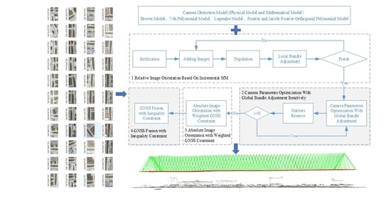
2.1. Camera Distortion Model

The classical Brown camera model in the field of photogrammetry and computer vision, the 7th polynomial model, and the Legendre, Fourier, and Jacobi–Fourier orthogonal polynomial models are compared and analyzed. The mathematical form of each camera distortion model is described below.

2.1.1. Brown Model

The Brown distortion model [10] has been widely used in the photogrammetry and computer vision field. The parameters of the Brown model mainly include symmetrical radial distortion, tangential distortion, and in-plane distortion [35,36]. The mathematical equations are as shown below.
Δ x = x ¯ ( k 1 r 2 + k 2 r 4 + k 3 r 6 ) + p 1 ( r 2 + 2 x ¯ 2 ) + 2 p 2 x ¯ y ¯ + b 1 x ¯ + b 2 y ¯ Δ y = y ¯ ( k 1 r 2 + k 2 r 4 + k 3 r 6 ) + p 1 ( r 2 + 2 y ¯ 2 ) + 2 p 2 x ¯ y ¯ r = ( x x 0 ) 2 + ( y y 0 ) 2 = x ¯ 2 + y ¯ 2
where x 0 , y 0 is the principal point of the image, k 1 , k 2 , k 3 are the radial distortion coefficients, p 1 , p 2 are the tangential distortion coefficients, and b 1 , b 2 are the in-plane distortion coefficients, which are named as the affinity and the shear terms. The in-plane coefficients represent different scaling factors and non-orthogonal pixels in the image along the x- and y-axis.

2.1.2. 7th Polynomial Model

The 7th polynomial camera distortion model is provided by the open-source software MicMac [25], and it contains a total of 66 parameters. The distortion functions are as follows:
Δ x = a 0 x ¯ + a 1 y ¯ 2 a 2 x ¯ 2 + a 3 x ¯ y ¯ + a 4 y ¯ 2 + a 6 x ¯ 3 + a 7 x ¯ 2 y ¯ + a 8 x ¯ y ¯ 2 + a 9 y ¯ 3 + a 14 x ¯ 4 + a 15 x ¯ 3 y ¯ + a 16 x ¯ 2 y ¯ 2 + a 17 x ¯ y ¯ 3 + a 18 y ¯ 4 + a 24 x ¯ 5 + a 25 x ¯ 4 y ¯ + a 26 x ¯ 3 y ¯ 2 + a 27 x ¯ 2 y ¯ 3 + a 28 x ¯ y ¯ 4 + a 29 y ¯ 5 + a 36 x ¯ 6 + a 37 x ¯ 5 y ¯ + a 38 x ¯ 4 y ¯ 2 + a 39 x ¯ 3 y ¯ 3 + a 40 x ¯ 2 y ¯ 4 + a 41 x ¯ y ¯ 5 + a 42 y ¯ 6 + a 50 x ¯ 7 + a 51 x ¯ 6 y ¯ + a 52 x ¯ 5 y ¯ 2 + a 53 x ¯ 4 y ¯ 3 + a 54 x ¯ 3 y ¯ 4 + a 55 x ¯ 2 y ¯ 5 + a 56 x ¯ y ¯ 6 + a 57 y ¯ 7 Δ y = a 0 y ¯ + a 1 x ¯ + a 2 x ¯ y ¯ 2 a 3 y ¯ 2 + a 5 x ¯ 2 + a 10 x ¯ 3 + a 11 x ¯ 2 y ¯ + a 12 x ¯ y ¯ 2 + a 13 y ¯ 3 + a 19 x ¯ 4 + a 20 x ¯ 3 y ¯ + a 21 x ¯ 2 y ¯ 2 + a 22 x ¯ y ¯ 3 + a 23 y ¯ 4 + a 30 x ¯ 5 + a 31 x ¯ 4 y ¯ + a 32 x ¯ 3 y ¯ 2 + a 33 x ¯ 2 y ¯ 3 + a 34 x ¯ y ¯ 4 + a 35 y ¯ 5 + a 43 x ¯ 6 + a 44 x ¯ 5 y ¯ + a 45 x ¯ 4 y ¯ 2 + a 46 x ¯ 3 y ¯ 3 + a 47 x ¯ 2 y ¯ 4 + a 48 x ¯ y ¯ 5 + a 49 y ¯ 6 + a 58 x ¯ 7 + a 59 x ¯ 6 y ¯ + a 60 x ¯ 5 y ¯ 2 + a 61 x ¯ 4 y ¯ 3 + a 62 x ¯ 3 y ¯ 4 + a 63 x ¯ 2 y ¯ 5 + a 64 x ¯ y ¯ 6 + a 65 y ¯ 7
where x ¯ , y ¯ are the same as the definition in the Brown model, and a 0 , a 1 , , a 65 are the coefficients of the 7th polynomial. Six coefficients are eliminated to reduce the correlation between those coefficients.

2.1.3. Legendre Model

The Legendre model is composed of a series of orthogonal polynomials, which greatly reduce the correlation between distortion coefficients. This model has been used in the camera self-calibration for professional digital mapping cameras. However, the feasibility of a consumer-grade camera applicated in camera self-calibration needs to be verified. Therefore, the Legendre orthogonal polynomial model with 66 parameters is introduced in this paper. The mathematical expression is presented in Formula (3), where p m , n = 10 6 l m ( x ¯ ) l n ( y ¯ ) , m , n [ 0 , 5 ] ; x ¯ = x w / 2 w , y ¯ = y h / 2 h ; x , y are the pixel coordinates in the image; and w and h represent the width and height of the image, respectively. l m ( x ¯ ) and l n ( y ¯ ) mean the Legendre polynomials and a 0 , a 1 , , a 65 are the coefficients. Similar to the 7th polynomial distortion model, six coefficients are eliminated in the Legendre model.
Δ x = a 0 p 1 , 0 + a 1 p 0 , 1 + a 2 p 2 , 0 + a 3 p 1 , 1 + a 4 p 0 , 2 + a 5 p 3 , 0 + a 6 p 2 , 1 + a 7 p 1 , 2 + a 8 p 0 , 3 + a 9 p 4 , 0 + a 10 p 3 , 1 + a 11 p 2 , 2 + a 12 p 1 , 3 + a 13 p 0 , 4 + a 14 p 5 , 0 + a 15 p 4 , 1 + a 16 p 3 , 2 + a 17 p 2 , 3 + a 18 p 1 , 4 + a 19 p 0 , 5 + a 20 p 5 , 1 + a 21 p 4 , 2 + a 22 p 3 , 3 + a 23 p 2 , 4 + a 24 p 1 , 5 + a 25 p 5 , 2 + a 26 p 5 , 3 + a 27 p 3 , 4 + a 28 p 2 , 5 + a 29 p 5 , 3 + a 30 p 4 , 4 + a 31 p 3 , 5 + a 32 p 5 , 4 + a 33 p 4 , 5 + a 34 p 5 , 5 Δ y = a 1 p 1 , 0 a 0 p 0 , 1 + a 35 p 2 , 0 a 2 p 1 , 1 a 3 p 0 , 2 + a 36 p 3 , 0 + a 37 p 2 , 1 + a 38 p 1 , 2 + a 39 p 0 , 3 + a 40 p 4 , 0 + a 41 p 3 , 1 + a 42 p 2 , 2 + a 43 p 1 , 3 + a 44 p 0 , 4 + a 45 p 5 , 0 + a 46 p 4 , 1 + a 47 p 3 , 2 + a 48 p 2 , 3 + a 49 p 1 , 4 + a 50 p 0 , 5 + a 51 p 5 , 1 + a 52 p 4 , 2 + a 53 p 3 , 3 + a 54 p 2 , 4 + a 55 p 1 , 5 + a 56 p 5 , 2 + a 57 p 5 , 3 + a 58 p 3 , 4 + a 59 p 2 , 5 + a 60 p 5 , 3 + a 61 p 4 , 4 + a 62 p 3 , 5 + a 63 p 5 , 4 + a 64 p 4 , 5 + a 65 p 5 , 5

2.1.4. Fourier Model

The mathematical formula of 16 parameters in the first-order orthogonal polynomial distortion model based on the two-dimensional Fourier series [21] is as follows:
Δ x f = a 0 c 1 , 0 + a 1 c 0 , 1 + a 2 c 1 , 1 + a 3 c 1 , 1 + a 4 s 1 , 0 + a 5 s 0 , 1 + a 6 s 1 , 1 + a 7 s 1 , 1 Δ y f = a 8 c 1 , 0 + a 9 c 0 , 1 + a 10 c 1 , 1 + a 11 c 1 , 1 + a 12 s 1 , 0 + a 13 s 0 , 1 + a 14 s 1 , 1 + a 15 s 1 , 1
where c m , n = 10 6 cos ( m x ¯ f + n y ¯ f ) , s m , n = 10 6 sin ( m x ¯ f + n y ¯ f ) , x ¯ f = x w / 2 w π , and y ¯ f = y h / 2 h π ; x , y are the pixel coordinates in the image; w and h represent the width and height of the image, respectively; and a 0 , a 1 , , a 15 are the coefficients. When there is significant radial distortion in the image, it needs to be employed together with the radial distortion model. Therefore, the radial distortion and quadratic polynomial are applied.
Δ x r g = x ¯ r ( k 1 r 2 + k 2 r 4 + k 3 r 6 ) + b 0 x ¯ g + b 1 y ¯ g 2 b 2 x ¯ 2 g + b 3 x ¯ g y ¯ g + b 4 y ¯ 2 g Δ y r g = y ¯ r ( k 1 r 2 + k 2 r 4 + k 3 r 6 ) b 0 y ¯ g + b 1 x ¯ g + b 2 x ¯ g y ¯ g 2 b 3 y ¯ 2 g g + b 5 x ¯ g 2
where x ¯ r , y ¯ r are consistent with x ¯ , y ¯ in the Brown model; x ¯ g = x ¯ f / π ,   y ¯ g = y ¯ f / π ; k 1 , k 2 , k 3 are the radial coefficients; and b 0 , b 1 , , b 5 are the coefficients of a quadratic polynomial. The final hybrid distortion model is as follows:
Δ x = Δ x f + Δ x r g Δ y = Δ y f + Δ y r g

2.1.5. Jacobi–Fourier Model

Compared with the Fourier model, the Jacobi–Fourier model has a higher horizontal and vertical accuracy [22]. In this paper, the Jacobi–Fourier model is adopted, and the function is presented in Formula (7), where J n ( α , β , r ) is the Jacobi polynomial and the mathematical expression is as shown in Formula (8); x ¯ , y ¯ [ 0 , 1 ] , represented as normalized image coordinates; r is the distance from the normalized pixel coordinate to the origin, r 2 = x ¯ 2 + y ¯ 2 ; N J , M F , N F  are the variable parameters of Jacobi and Fourier, respectively; and a i , m , n , b i , m , n , a i , m , n , b i , m , n are the coefficients of the polynomial.
Δ x j f = i = 0 N J m = 0 M F n = 1 N F a i , m , n J i ( α , β , r ) sin ( m π x ¯ + n π y ¯ ) + i = 0 N J m = 0 M F n = 1 N F b i , m , n J i ( α , β , r ) cos ( m π x ¯ + n π y ¯ ) Δ y j f = i = 0 N J m = 0 M F n = 1 N F a i , m , n J i ( α , β , r ) sin ( m π x ¯ + n π y ¯ ) + i = 0 N J m = 0 M F n = 1 N F b i , m , n J i ( α , β , r ) cos ( m π x ¯ + n π y ¯ )
J n ( α , β , τ ) = ω ( α , β , τ ) b n ( α , β ) · τ G n ( α , β , τ ) G n ( α , β , τ ) = n ! ( β 1 ) ! ( α + n 1 ) ! s = 0 n ( 1 ) s ( α + n + s 1 ) ! ( n s ) ! s ! ( β + s 1 ) ! τ s b n ( α , β ) = n ! [ ( β 1 ) ! ] 2 ( α β + n ) ! ( β + n 1 ) ! ( α + n 1 ) ! ( α + 2 n ) ω ( α , β , τ ) = ( 1 τ ) α β τ β 1
In Formula (8), α , β are set to 7 and 3, respectively, according to the suggestion of [22]; τ [ 0 , 1 ] , and G n , b n , ω are the polynomial, normalizing constant, and weighting function, respectively. Similar to the Fourier model, the Jacobi–Fourier model is mixed with radial distortion and quadratic polynomial as given in the following.
Δ x = Δ x j f + Δ x r g Δ y = Δ y j f + Δ y r g

2.2. GNSS-Aided Bundle Adjustment with Inequality Constraint

GNSS-aided BA is the commonly used method in the photogrammetry and computer vision fields. By minimizing the reprojection error, the traditional BA can optimize the internal and external parameters of the camera together with the 3D coordinates of the tie points. The error equation of GNSS-aided BA considers the deviation between the image projection center X c and GNSS phase center X g p s . The jointly optimized error function is as described in Formula (10), where w is the weight of GNSS.
e u = j ρ j ( | | π ( P c , X k ) x j | | 2 2 ) + n ρ n ( | | w ( X c X g p s | | 2 2 )
Different from the traditional weighted GNSS-aided BA, Maxime et al. [33] proposed an inequality constrained bundle adjustment (IBA) method with GNSS fusion to reduce the deviation error accumulation between the image projection center X c and the GNSS location X g p s for long image sequences. The basic idea of IBA is to improve the absolute accuracy with GNSS-aided BA on the premise of appropriately increasing the reprojection error. Let X = ( X c T , X a T , X k T ) be the optimal solution of standard BA without consideration of GNSS information, where X c , X a , X k represent the projection center of image, rotation angle, and 3D coordinates of tie points, respectively. Further, let e ( X ) be the minimum sum of square reprojection errors with the optimal solution, i.e., X , e ( X * ) e ( X ) . Suppose e t be a threshold that is slightly larger than the minimum reprojection error e ( X ) , i.e., e ( X ) < e t . IBA assumes that the GNSS error is bounded and the reprojection error e ( X ) of BA with GNSS constraint should be less than e t , that is, e ( X ) e t . Under this condition, the optimized image projection center should be as close to the GNSS phase center as possible, i.e., X c X g p s .
Let X 2 = ( X a , X k ) , then the unknowns of BA can be expressed as X = ( X c T , X 2 T ) . Let P = ( I , 0 ) be such that X c = P X . IBA establishes the optimization equation by combining penalty function and inequality constraint, as shown in Formula (11).
e I ( X ) = γ c I ( X ) + | | P X X g p s | | 2
where γ is a user-defined weight and a positive number, c I ( X ) = e t e ( X ) , and c I ( X ) > 0 . The objective function is iteratively minimized by this inequality and penalty function γ / c I ( X ) constraint. The penalty function value is close to positive infinity in the neighborhood of c I = 0 . The algorithm in C style is shown in Algorithm 1 and the parameter γ is set γ = e t e ( X * ) 10 | | P X * X g p s | | 2 according to [33]. More details should be referenced in [33].
Algorithm 1 The procedure of IBA
1:  e r r = γ / ( e t e ( X ) ) + | | P X X g p s | | 2
2: UpdateD = 1;  λ = 0.001 ;
3: for (It = 0; It < I t max ; It++) {
4:  if (UpdateD) {
5:  UpdateD = 0;
6:   g = 2 J T E ( X ) ; H = 2 J T J ;
7:   g I = γ ( e t e ) 2 g + 2 P T ( P X X g p s ) ; H = γ ( e t e ) 2 H + 2 P T P ;
8:   g ˜ = 2 γ ( e t e ) 3 g ;
9:  }
10:   H ~ = H + λ d i a g ( H + g ~ g ~ T )
11:   s o l v e H ~ ( a , b ) = ( g , g ~ ) ;
12:   Δ = a g ~ T a 1 + g ~ T b b ;
13:  if ( e ( X + e t ) {
14:   λ = 10 λ ; continue;
15:  }
16:   e r r = γ e t e ( X + ) + | | P ( X + ) X g p s | | 2 ;
17:  if ( e r r < e r r ) {
18:   X = X + ;
19:  if ( 0.9999 e r r < e r r ) break;
20:   e r r = e r r ; UpdateD = 1; λ = λ / 10 ;
21:  } else
22:   λ = 10 λ ;
23:}

2.3. Camera Self-Calibration for Long Corridor UAV Images

The camera self-calibration for long corridor UAV images is realized under the framework of incremental SfM in ColMap. Firstly, the incremental SfM selects two seed images with enough matching feature points, which are of uniform distribution in the images and the intersection angle between the two-image pair should be large enough. Then the relative orientation and 3D coordinates of tie points in the initial image pair are calculated. Secondly, the next best images are selected, which are most fully connected with the existing reconstructed model. The image poses and 3D coordinates of tie points are recovered immediately. Finally, to eliminate accumulated error, the local and global BA optimization is carried out iteratively: (1) when the number of newly added images exceeds a given threshold, local BA optimization is performed for the local-oriented images; (2) when the percentage of registered images grows by a certain threshold, the reconstructed model is optimized by global BA [37]. The feature point extraction, exhaustive matching strategy, criteria for seed image selection, and the strategies of controlling local BA in ColMap are directly used in the proposed method without any changes.
For the long corridor UAV images, the existing incremental SfM framework has the following shortcomings:
  • From the perspective of camera self-calibration, the next best image selection does not consider whether the scene structure is degraded. If the structure of the seed image is poor and lacks height variation, the camera intrinsic parameters are unstable and may even lead to the failure of the final reconstruction.
  • At present, UAV images often record high-precision GNSS location information, which can alleviate the “bowl effect” of long corridor images. The existing incremental SfM framework of camera self-calibration does not take full advantage of GNSS information for absolute orientation.
  • The inaccurately estimated distortion parameters have an adverse impact on the 3D point clouds generated by dense matching technology. The power lines in UAV images of high-voltage transmission are usually 1~2 pixels in width. When the distortion parameters are estimated inaccurately, the reconstructed point clouds of power lines are noisy and diverged around. Figure 3 shows the dense point clouds reconstructed by ColMap with inaccurate camera distortion parameters.
Therefore, a camera self-calibration method is proposed, which combines the camera parameters initialization and high-precision differential GNSS position information fusion. The workflow is shown in Figure 4, and details of key steps are listed as follows:
  • Image-relative orientation based on incremental SfM framework. Only the local BA is performed to reduce the error accumulation, and the focal length, principal point, and distortion parameters of the image are kept fixed to avoid the problem of the unstable and large variation of distortion parameters and focal length caused by the instability structure of image and scene degradation. The results of image-relative orientation are shown in Figure 5a.
  • Global BA and iterative optimization of camera parameters. In the process of iterative global BA and gross error elimination, the optimization strategy of gradually freeing the intrinsic and distortion of camera parameters is adopted, that is, (a) distortion parameters, (b) focal length, and (c) principal point. This strategy can alleviate the correlation between focal length, principal point, and distortion parameters of the camera. According to the experiment, when the number of iterations is bigger than two, the camera intrinsic parameters become stable. In this paper, the global BA is iterated three times. In each iteration, the distortion, focal length, and principal point parameters of the camera are optimized using the strategy of gradually freeing parameters, to provide better initial values for GNSS-constrained BA.
  • Traditional weighted GNSS-constrained absolute orientation. At this time, the GNSS-constrained BA optimizes the focal length, principal point, and distortion parameters as unknowns together. Further, the error equation is shown in Formula (12).
e u = j ρ j ( | | π ( P c , X k , θ ) x j | | 2 2 ) + n ρ n ( | | w ( X c X g p s | | 2 2 )
where θ = ( f , c x , c y , D i s t ) , including the focal length f, principal point c x , c y , and the distortion parameters D i s t . The distortion parameters D i s t are determined by the selected camera distortion model introduced in Section 2.1. The weight of GNSS w is set to 10, keeping consistent with [33]. The cost function ρ is the Cauchy function with stronger noise resistance, as shown in Formula (13).
ρ ( s ) = log ( 1 + s )
4.
GNSS fusion based on IBA. This paper combines IBA to further fuse the GNSS. The main steps are as follows: (a) the camera focal length, principal point, and distortion parameters are used as unknowns to optimize together during camera self-calibration; (b) the initial input parameters e ( X ) are the sum of the squares’ reprojection error of weighted GNSS-constrained BA, and X * are the minimum solvers; (c) all the image projection centers and the corresponding GNSS positions are used as constraints for global IBA to solve iteratively. The final reconstructed model with the proposed camera self-calibration strategy is shown in Figure 5b.
In summary, there are several differences between the proposed method with the incremental SfM in ColMap and the usage of IBA in [33]. In ColMap, the local BA is performed on the images that are connected with the most recently registered images, and the global BA is performed according to the growing percentage of the registered images. The camera intrinsic parameters are optimized during local BA and global BA. In the proposed method, only local BA is performed before all images are registered, and the global BA is literately performed after all images are registered. During the local BA, the camera intrinsic parameters are kept fixed. Further, during the global BA, the camera intrinsic parameters are gradually freed to get better initial values. Then the traditional weighted and inequality constrained BA with GNSS is performed for absolute orientation. In [33], the IBA is used in local BA to fuse the low-cost GNSS and image projection centers to refine the k-most recent images. The input-optimized initial parameters are the results of local BA and the 3D GNSS location of the corresponding most recent image. The camera intrinsic parameters are known and kept fixed. In the proposed method, the IBA is used in global BA to fuse high-precision GNSS locations and image projection centers. The camera intrinsic parameters are freed and optimized together with the GNSS constraint. The inputs of IBA in the proposed method are the optimized parameters of the weighted GNSS constraint BA and all the GNSS locations of registered images. The differences between the proposed method and the incremental SfM in ColMap and the IBA in [33] are listed in Table 1 and Table 2, respectively.

3. Results and Discussion

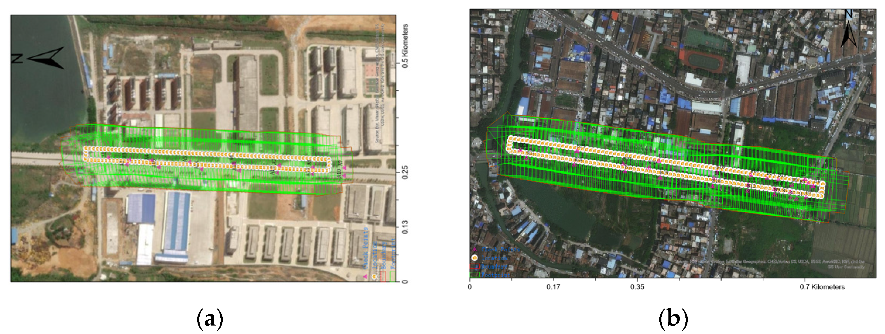
3.1. Test Sites and Datasets

Two datasets of long corridor transmission line UAV images were collected by DJI Phantom 4 RTK UAV, as shown in Figure 6. Figure 6a,b was collected using the rectangle closed-loop trajectory; Figure 6c,d was collected using the S-shaped strip trajectory. The rectangle and S-shaped trajectories were made by a third-party software developed based on DJI Mobile SDK, and during the flight, the standard control algorithm provided by DJI was applied to fly and take photos in autonomous mode along the trajectories. For the rectangle trajectories, the forward and side overlap ratio of images were set to 88% and 75%, respectively, and the flight speed was set to 4 m/s. For the S-shaped trajectories, the forward and side overlap ratio of images were set to 82% and 61%, respectively, and the flight speed was set to 6 m/s. The time interval for taking photos was 3 s for all flights. The camera focal length was kept fixed during image collection. The UAV flight height was set to 70 m, which is relative to the position from where the UAV takes off and the camera takes images vertically downward. The GSD (ground resolution distance) of images was 2.1 cm. The numbers of each image datasets were 140, 166, 165, and 132, respectively. To verify the absolute orientation accuracy of BA, the accurate ground coordinates in the two test sites were collected by Hi-Target iRTK2 GNSS receiver and FindCM CORS. The targets were marked with red paint manually on the road using the perpendicular lines with a width of about 10 cm, and the ground coordinates inside the right angle were measured. Finally, 15 targets were collected in test site 1 and 27 targets were collected in test site 2. The distribution of targets is listed in Figure 6e,f. The targets in test site 1 were labeled from A1 to A15, and the targets in test site 2 were labeled from B1 to B27. For the experiments of camera self-calibration without GCP constraint, all the targets were regarded as check points to evaluate the accuracy. For the experiments with one GCP constraint, the target of A14 in test site 1 and the target of B20 in test site 2 were regarded as control points and the rest of the targets were regarded as check points for accuracy evaluation. Both A14 and B20 were located in the middle of the long corridors.

3.2. Analysis of the Influence of Camera Distortion Models

Firstly, the influence of different image acquisition modes and camera distortion models on the accuracy of bundle block adjustment was analyzed. For the hybrid Fourier and Jacobi–Fourier models, the radial and quadratic polynomial distortion parameters were first calculated with all images. Then, we kept these parameters fixed and calculated the parameters of Fourier and Jacobi–Fourier. For other distortion models, all the distortion parameters were calculated at one time. The mean, SD (standard deviation), and RMSE (root mean square error) were used to evaluate the accuracy of checkpoints.
The statistical results are listed in Table 3. Figure 7 and Figure 8 show the residuals of check points for different distortion models. It can be seen that the accuracy of S-shaped image datasets was significantly better than that of rectangle image datasets (except for the vertical accuracy of the Brown model and hybrid Jacobi–Fourier model in test site 2). The main reason is that when the images are collected in the S-shaped method, the angle between the images is always changing, which can reduce the correlation between distortion and other parameters of the camera, and then the horizontal accuracy and vertical accuracy are improved.
For further analysis, we can see the following: (1) For the rectangle dataset of test site 1, the horizontal and vertical accuracy with the Brown model was higher than other distortion models. However, for the other three datasets, the accuracy of the Brown model was the worst. (2) From the comparison of camera self-calibration between the Poly7 model and the Legendre model, it can be seen that the horizontal accuracy of Poly7 was better than the Legendre model for all the datasets. Further, the Poly7 model had better vertical accuracy in the S-shaped dataset of test site 2. However, the Legendre model had better vertical accuracy than the Poly7 model in the other three datasets. The main reason is that the orthogonality of the Legendre model can improve the accuracy of focal length for camera self-calibration, and then improve the vertical accuracy, but meanwhile, it loses the horizontal accuracy. (3) From the comparison of camera self-calibration between the hybrid Fourier model and hybrid Jacobi–Fourier model, it can be seen that the horizontal accuracy of the two models had little difference. However, the vertical accuracy of the hybrid Jacobi–Fourier model was better than the hybrid Fourier model in general (except for the S-shaped dataset in test site 2).
In summary, the bundle block adjustment accuracy in the horizontal direction with the five different models can reach the centimeter level, while the vertical accuracy has great differences for the four datasets. No one distortion model can achieve the best accuracy among all four datasets. Overall, the horizontal and vertical accuracy of bundle block adjustment with mathematical distortion models was better than the physical model in the long corridor structure datasets, and the vertical accuracy of the hybrid Jacobi–Fourier model was generally better than the other three mathematical distortion models.

3.3. Analysis of the Performance of Proposed Self-Calibration

To verify the feasibility of the proposed strategy for camera self-calibration, this paper is compared with the scheme of ColMap [38]. Since ColMap does not implement the GNSS-constrained BA, the similarity transforms were applied for the projection center of images and GNSS after the final global BA in ColMap. Then, the weighted BA with GNSS as described in Formula (12) was conducted. Considering that ColMap does not provide any mathematical distortion models, the Brown model was adopted to make the experimental comparison.
The statistical results of check points after camera self-calibration are shown in Table 4. The results show that the horizontal accuracy with the proposed strategy is better than that of ColMap’s in the four datasets of the two test sites. In the direction of elevation, the proposed strategy significantly improved the RMSE accuracy than ColMap (except for the rectangle dataset in test site 2). Due to the “bowl effect” in ColMap camera self-calibration, although its mean value was smaller than that of the proposed strategy in the S-shaped dataset of test site 1, it had a large standard deviation, which indicates that there is a large fluctuation in the vertical direction of the reconstructed model with ColMap, as shown in Figure 9b. In the rectangle dataset of test site 2, the elevation of ColMap had a higher accuracy in the mean and RMSE than that of the proposed strategy. The reason is that the initial image pair selected during the incremental SfM framework had a better structure, which led to a smaller variation range of focal length and a higher accuracy. However, it should be noted that the standard deviation of ColMap in this dataset was 0.055 larger than ours, which shows that the ColMap’s fluctuation of elevation error is still large and there is a “bowl effect” in the reconstructed model with a certain bending phenomenon, as shown in Figure 9c. In conclusion, the proposed camera self-calibration strategy had advantages in horizontal accuracy and had better vertical accuracy than ColMap in three of the datasets.
The DJI Phantom 4 RTK UAV records the differential GNSS location of the image with centimeter positioning accuracy. The relative accuracy between the projection center of the image after camera self-calibration with the proposed strategy and the corresponding GNSS location were analyzed. As the horizontal relative errors between the proposed method and ColMap had no obvious regularity and the vertical relative errors can indicate whether the “bowl effect” appears, the vertical offset distribution of the image projection centers after camera self-calibration and the corresponding GNSS locations in the four datasets are listed in Figure 9. It can be seen that, in the elevation direction, the reconstructed model of ColMap had obvious bending. It is a convex shape that is higher in the middle and lower on both sides in the rectangle dataset of test site 1. Further, it shows a concave shape that is lower in the middle and higher on both sides in both the S-shaped dataset of test site 1 and the rectangle dataset of test site 2. The offsets in the vertical direction of the reconstructed model with the proposed method are small, which significantly alleviates the “bowl effect”. For the S-shaped dataset of test site 2, there are two broken jumps in the proposed method and ColMap. The main reason is that the large illumination leads to the increase of mismatch feature points, which affects the accuracy of bundle block adjustment. In summary, the vertical relative accuracy of the proposed method in the vertical direction is significantly improved compared with ColMap and the bending of the reconstructed model is reduced.

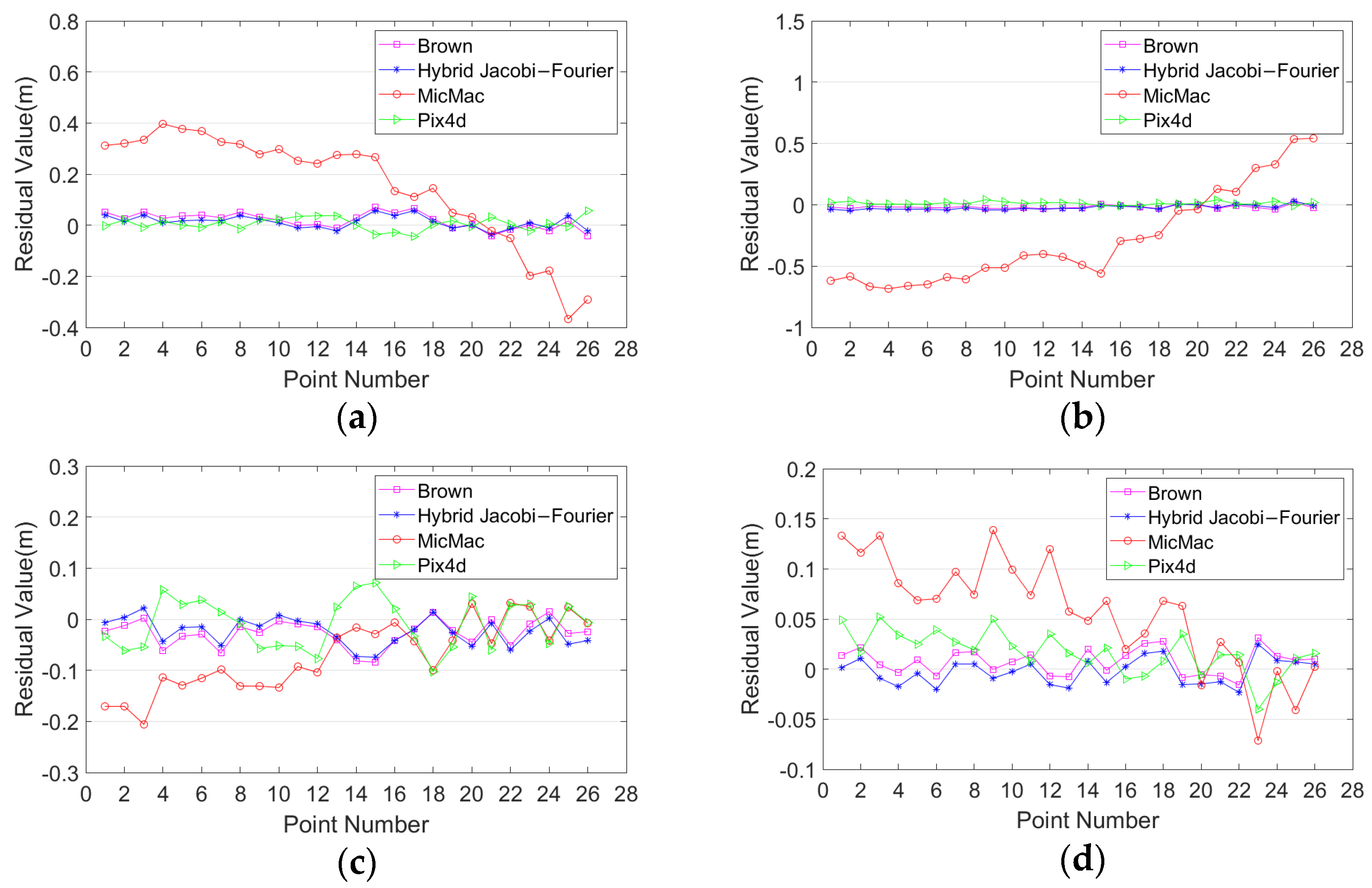
3.4. Comparison with State-Of-The-Art Software

The open-source software MicMac and the commercial software Pix4d Mapper were selected to compare and analyze with the proposed method. Based on the comparative experiments mentioned above with different distortion models, it was found that the overall performance of the hybrid Jacob–Fourier model was the best. Therefore, the hybrid Jacobi–Fourier distortion model was selected for further comparative analysis. The F15P7 distortion model was adopted in MicMac with the strategies proposed in [25]. The distortion model of Pix4d Mapper was unknown. In this section, self-calibration is conducted without and with GCPs.

3.4.1. Bundle Adjustment without GCP

For bundle adjustment without GCP, the experimental results are listed in Table 5. Figure 10 and Figure 11 show the residual of check points with this software after camera self-calibration. From the analysis of horizontal accuracy, the following can be seen: (1) The proposed method had the smallest mean value in the two datasets of test site 1. The mean values of Pix4d in both datasets of test site 2 are the smallest. For the two datasets of test site 1, the standard deviation of MicMac in the Y direction is the largest, reaching 0.1 m, while Pix4d and the proposed method are both less than 0.07 m. Therefore, MicMac performs the worst overall. (2) The RMSE values in the X direction of Pix4d and the proposed method have little difference in the datasets except for the S-shaped dataset of test site 1. However, the RMSE values of Pix4d in the Y direction are 0.03 m, 0.015 m, and 0.010 m larger than the proposed method. Therefore, the horizontal accuracy of the proposed method is generally better than Pix4d.
From the analysis of the vertical accuracy, the following can be seen: (1) The proposed method had the smallest standard deviation in the datasets except for the S-shaped dataset of test site 2. Pix4d had the smallest standard deviation in the S-shaped dataset of test site 2. MicMac had the largest standard deviation in the four datasets and the accuracy fluctuates greatly. (2) For test site 1, the RMSE values of MicMac were the smallest, but it had the largest standard deviation and the reconstructed model had obvious bending, as shown in Figure 12a,b. Pix4d had the smallest RMSE and standard deviation in the S-shaped dataset of test site 2. The possible reason is that the feature points matching of Pix4d is more robust with the large change of illumination. However, the RMSE values of Pix4d in the vertical direction were 0.787 m, 0.324 m, and 0.74 m larger than the proposed method, which indicates that the proposed has better accuracy in the vertical direction. To sum up, compared with MicMac and Pix4d, the proposed method still has certain advantages.
To evaluate the “bowl effect” with different software, the relative errors in the Z direction between the projection centers and the corresponding GNSS locations are shown in Figure 12. Compared with Pix4d and the proposed method, MicMac had the worst performance in the vertical relative accuracy between the projection centers and GNSS locations. The fluctuation range of vertical relative errors was between −0.2 m and 0.3 m with MicMac, which is much bigger than Pix4d and the proposed method. There was a “bowl effect” with MicMac in the four datasets except for the S-shaped dataset in test site 2, while the bending of the reconstructed models was significantly reduced with Pix4d and the proposed method. The vertical relative errors of the proposed method were close to Pix4d. The “bowl effect” was alleviated with the proposed method and Pix4d.

3.4.2. Bundle Adjustment with GCP

For bundle adjustment with GCP, a single GCP was applied for the camera self-calibration experiment compared with MicMac and Pix4d Mapper. All the optimized parameters of Section 3.4.1 were used as the initial parameters for MicMac and the proposed method with one single GCP-constrained BA. The Brown and hybrid Jacobi–Fourier distortion models were selected with the proposed method. Table 6 lists the experimental results. Figure 13 and Figure 14 show the residuals of check points after camera self-calibration with one single GCP. From the analysis of horizontal accuracy, the accuracy of the Brown and hybrid Jacobi–Fourier distortion models with the proposed strategy is comparable. The mean values in the horizontal direction of X and Y with MicMac were the largest in the datasets except for the S-shaped dataset of test site 1, and the horizontal RMSE values and standard deviation values were also the largest among the four datasets. In the two datasets of test site 1, the mean values and RMSE values of Pix4d in the X and Y horizontal directions were larger than the Brown and hybrid Jacobi–Fourier model. Further, in the two datasets of the test site 2, the mean values and RMSE values of Pix4d in the horizontal direction of X were smaller than Brown and hybrid Jacobi–Fourier model with the proposed strategy, but in the Y direction, they were larger than the two distortion models with the proposed strategy. In general, the horizontal accuracy of the proposed method is relatively close to Pix4d. The horizontal RMSE value of the two distortion models with the proposed method was better than 0.04 m, while MicMac was less than 0.5 m and Pix4d was less than 0.08 m.
From the analysis of elevation, the two distortion models with the proposed strategy achieved the best accuracy, while MicMac achieved the worse. The RMSE in the vertical direction of MicMac was greater than 0.1 m, while Pix4d was less than 0.1 m and the two distortion models with the proposed strategy were both less than 0.05 m. The vertical accuracy of the two distortion models was relatively close, and the difference between the first three datasets was only at the millimeter level, while the vertical RMSE of the hybrid Jacobi–Fourier model was 0.01 m better than the Brown in the S-shaped dataset of test site 2. Therefore, in the case of a single GCP constraint, the accuracy of the Brown model is comparable to the hybrid Jacobi–Fourier model, and the overall accuracy of camera self-calibration with the proposed strategy is better than that of MicMac and Pix4d. Additionally, compared with Table 5 in the vertical direction, MicMac had the smallest RMSE value in the rectangle dataset of test site 1 while Pix4d had the smallest RMSE value in the S-shaped dataset of test site 2. However, the vertical RMSE of Brown and hybrid Jacobi–Fourier models with the proposed strategy was better than MicMac and Pix4d after adding a single GCP. The reason is that the horizontal accuracy is ensured and the relative errors between image projection centers and GNSS locations are small with the experiments of direct georeferencing in Section 3.3 and Section 3.4.1, which indicates that the proposed method can significantly reduce the bending of the reconstructed model and the image structures have litter distortion. The “bowl effect” is alleviated. The only problem is that the vertical accuracy is unstable because the focal length is highly correlated with other distortion parameters. With one GCP constraint, the correlation between focal length and other distortion parameters is reduced and the focal length can be accurately estimated. In this case, vertical accuracy can be ensured.

4. Conclusions

The UAV images collected on a linear axis and fixed height are critical configurations for camera self-calibration, which may lead to the “bowl effect”. To solve such a tough problem, traditional methods rely on more than three GPCs, while the proposed method relies on only one GCP. The proposed new camera self-calibration method for long corridor UAV images in high transmission lines combines the initialization of the camera calibration parameters and the fusion of high-precision differential GNSS position information for long corridor UAV images in high transmission lines. Based on the comprehensive analysis of the physical and mathematical models of camera distortion, the new camera self-calibration method was designed, which takes full consideration of the initialization of the camera intrinsic parameters in long corridor UAV images and the fusion of differential GNSS with inequality constrained BA.
The UAV images of two test sites with two different acquisition modes were applied for camera self-calibration experiments. The experimental results show that the proposed camera self-calibration method can significantly alleviate the “bowl effect” for long corridor UAV images, reduce the bending of the reconstructed model, and improve the absolute accuracy. Compared to the accuracy using the physical distortion model without any GCPs, the mathematical distortion models achieve better horizontal and vertical accuracy in the weak structure datasets. Among them, the vertical accuracy of the hybrid Jacobi–Fourier distortion model is generally better than the other mathematical models. Furthermore, with only one single GCP constraint, the proposed method with Brown and hybrid Jacobi–Fourier distortion models achieved the best accuracy compared with open-source and commercial software. Compared with the open-source software MicMac, the RMSEs in the directions of X, Y, and Z improved the GSD value on average approximately 8.36, 4.02, and 7.07 times, respectively, in the four datasets with the Brown model, and improved the GSD value on average approximately 8.18, 4.05, and 7.12 times, respectively, with hybrid Jacobi–Fourier model. Compared with the commercial software Pix4d, the RMSEs in the directions of X, Y, and Z improved the GSD value on average approximately 0.08, 0.80, and 0.85 times, respectively in the four datasets with the Brown model. Although, in the direction of X, the RMSE lost 0.01 times the GSD value with the hybrid Jacobi–Fourier model, while the RMESs in the directions of Y and Z improved 0.82 and 0.94 times the GSD value on average, respectively. Considering that different distortion models perform differently with different scenes, this study focuses on how to select the appropriate distortion model according to the characteristics and uncertainty of the scene in future work.

Author Contributions

W.H. and W.J. conceived and designed the experiments; W.H. and S.J. performed the experiments; W.J. collected the data; S.J. and W.H. wrote the manuscript; W.J. revised the manuscript. All authors have read and agreed to the published version of the manuscript.

Funding

This research was funded by the National Natural Science Foundation of China (Grant No. 42001413), Nature Science Foundation of Hubei Province (Grant No. 2020CFB324), the Open Fund of State Laboratory of Information Engineering in Surveying, Mapping and Remote Sensing, Wuhan University (Grant No. 20E03).

Institutional Review Board Statement

Not applicable.

Informed Consent Statement

Not applicable.

Data Availability Statement

Data available on request due to restrictions, e.g., privacy or ethical. The data presented in this study are available on request from the corresponding author. The data are not publicly available due to [the policy to protect the coordinates of pylon].

Conflicts of Interest

The authors declare no conflict of interest.

References

  1. Xiang, T.-Z.; Xia, G.-S.; Zhang, L. Mini-unmanned aerial vehicle-based remote sensing: Techniques, applications, and prospects. IEEE Geosci. Remote Sens. Mag. 2019, 7, 29–63. [Google Scholar] [CrossRef] [Green Version]
  2. Jiang, S.; Jiang, W.; Huang, W.; Yang, L. UAV-Based Oblique Photogrammetry for Outdoor Data Acquisition and Offsite Visual Inspection of Transmission Line. Remote Sens. 2017, 9, 278. [Google Scholar] [CrossRef] [Green Version]
  3. Jiang, S.; Jiang, W. UAV-based Oblique Photogrammetry for 3D Reconstruction of Transmission Line: Practices and Applications. In Proceedings of the International Archives of the Photogrammetry, Remote Sensing & Spatial Information Sciences, Enschede, The Netherlands, 10–14 June 2019; pp. 401–406. [Google Scholar]
  4. Zhang, H.; Yang, W.; Yu, H.; Zhang, H.; Xia, G.-S. Detecting power lines in UAV images with convolutional features and structured constraints. Remote Sens. 2019, 11, 1342. [Google Scholar] [CrossRef] [Green Version]
  5. Zhang, Y.; Yuan, X.; Li, W.; Chen, S. Automatic Power Line Inspection Using UAV Images. Remote Sens. 2017, 9, 824. [Google Scholar] [CrossRef] [Green Version]
  6. Huang, W.; Jiang, S.; Jiang, W. A Model-Driven Method for Pylon Reconstruction from Oblique UAV Images. Sensors 2020, 20, 824. [Google Scholar] [CrossRef] [Green Version]
  7. Triggs, B. Autocalibration from Planar Scenes. In Proceedings of the European Conference on Computer Vision, Berlin, Germany, 2–6 June 1998; pp. 89–105. [Google Scholar]
  8. Zhang, Z. A Flexible New Technique for Camera Calibration. IEEE Trans. Pattern Anal. Mach. Intell. 2000, 22, 1330–1334. [Google Scholar] [CrossRef] [Green Version]
  9. Oniga, E.; Pfeifer, N.; Loghin, A.-M. 3D Calibration Test-Field for Digital Cameras Mounted on Unmanned Aerial Systems (UAS). Remote Sens. 2018, 10, 2017. [Google Scholar] [CrossRef] [Green Version]
  10. Duane, C.B. Close-Range Camera Calibration. Photogramm. Eng. 1971, 37, 855–866. [Google Scholar]
  11. Fraser, C.S. Digital camera self-calibration. ISPRS J. Photogramm. Remote Sens. 1997, 52, 149–159. [Google Scholar] [CrossRef]
  12. Luhmann, T.; Robson, S.; Kyle, S.; Harley, I.A. Close Range Photogrammetry: Principles, Techniques and Applications; Whittles Publishing: Dunbeath, Caithness, Scotland, 2006; Volume 3. [Google Scholar]
  13. Fitzgibbon, A.W. Simultaneous Linear Estimation of Multiple View Geometry and Lens Distortion. In Proceedings of the IEEE Computer Society Conference on Computer Vision and Pattern Recognition, Kauai, HI, USA, 8–14 December 2001; p. I. [Google Scholar]
  14. Kukelova, Z.; Pajdla, T. A Minimal Solution to the Autocalibration of Radial Distortion. In Proceedings of the IEEE Conference on Computer Vision and Pattern Recognition, Minneapolis, MN, USA, 17–22 June 2007; pp. 1–7. [Google Scholar]
  15. Kukelova, Z.; Pajdla, T. A Minimal Solution to Radial Distortion Autocalibration. IEEE Trans. Pattern Anal. Mach. Intell. 2011, 33, 2410–2422. [Google Scholar] [CrossRef]
  16. Jiang, F.; Kuang, Y.; Solem, J.E.; Åström, K. A Minimal Solution to Relative Pose with Unknown Focal Length and Radial Distortion. In Proceedings of the Asian Conference on Computer Vision, Singapore, 1–5 November 2014; pp. 443–456. [Google Scholar]
  17. Kukelova, Z.; Heller, J.; Bujnak, M.; Fitzgibbon, A.; Pajdla, T. Efficient Solution to the Epipolar Geometry for Radially Distorted Cameras. In Proceedings of the 2015 IEEE International Conference on Computer Vision, Santiago, Chile, 11–18 December 2015; pp. 2309–2317. [Google Scholar]
  18. Ebner, H. Self calibrating block adjustment. Bildmess. Und Luftbildwessen 1976, 44, 128–139. [Google Scholar]
  19. Gruen, A. Accuracy, reliability and statistics in close-range photogrammetry. In Proceedings of the Inter-Congress Symposium of ISP Commission V, Stockholm, Sweden, 14–17 August 1978. [Google Scholar]
  20. Tang, R.; Fritsch, D.; Cramer, M.; Schneider, W. A Flexible Mathematical Method for Camera Calibration in Digital Aerial Photogrammetry. Photogramm. Eng. Remote Sens. 2012, 78, 1069–1077. [Google Scholar] [CrossRef]
  21. Tang, R.; Fritsch, D.; Cramer, M. New rigorous and flexible Fourier self-calibration models for airborne camera calibration. ISPRS J. Photogramm. Remote Sens. 2012, 71, 76–85. [Google Scholar] [CrossRef]
  22. Babapour, H.; Mokhtarzade, M.; Valadan Zoej, M.J. Self-calibration of digital aerial camera using combined orthogonal models. ISPRS J. Photogramm. Remote Sens. 2016, 117, 29–39. [Google Scholar] [CrossRef]
  23. Wu, C. Critical Configurations for Radial Distortion Self-Calibration. In Proceedings of the 2014 IEEE Conference on Computer Vision and Pattern Recognition, Columbus, OH, USA, 28 June 2014; pp. 25–32. [Google Scholar]
  24. Zhou, Y.; Rupnik, E.; Meynard, C.; Thom, C.; Pierrot-Deseilligny, M. Simulation and Analysis of Photogrammetric UAV Image Blocks—Influence of Camera Calibration Error. Remote Sens. 2019, 12, 22. [Google Scholar] [CrossRef] [Green Version]
  25. Tournadre, V.; Pierrot-Deseilligny, M.; Faure, P.H. UAV Linear Photogrammetry. In Proceedings of the International Archives of Photogrammetry, Remote Sensing and Spatial Information Sciences, La Grande Motte, France, 28 September–3 October 2015; p. 327. [Google Scholar]
  26. Polic, M.; Steidl, S.; Albl, C.; Kukelova, Z.; Pajdla, T. Uncertainty based camera model selection. In Proceedings of the IEEE/CVF Conference on Computer Vision and Pattern Recognition, Seattle, WA, USA, 16–18 June 2020; pp. 5991–6000. [Google Scholar]
  27. Griffiths, D.; Burningham, H. Comparison of pre- and self-calibrated camera calibration models for UAS-derived nadir imagery for a SfM application. Prog. Phys. Geogr. Earth Environ. 2018, 43, 215–235. [Google Scholar] [CrossRef] [Green Version]
  28. Jaud, M.; Passot, S.; Le Bivic, R.; Delacourt, C.; Grandjean, P.; Le Dantec, N. Assessing the accuracy of high resolution digital surface models computed by PhotoScan® and MicMac® in sub-optimal survey conditions. Remote Sens. 2016, 8, 465. [Google Scholar] [CrossRef] [Green Version]
  29. Salach, A.; Bakuła, K.; Pilarska, M.; Ostrowski, W.; Górski, K.; Kurczyński, Z. Accuracy assessment of point clouds from LiDAR and dense image matching acquired using the UAV platform for DTM creation. ISPRS Int. J. Geo-Inf. 2018, 7, 342. [Google Scholar] [CrossRef] [Green Version]
  30. Jaud, M.; Passot, S.; Allemand, P.; Le Dantec, N.; Grandjean, P.; Delacourt, C. Suggestions to limit geometric distortions in the reconstruction of linear coastal landforms by SfM photogrammetry with PhotoScan® and MicMac® for UAV surveys with restricted GCPs pattern. Drones 2019, 3, 2. [Google Scholar] [CrossRef] [Green Version]
  31. Nahon, A.; Molina, P.; Blázquez, M.; Simeon, J.; Capo, S.; Ferrero, C. Corridor mapping of sandy coastal foredunes with UAS photogrammetry and mobile laser scanning. Remote Sens. 2019, 11, 1352. [Google Scholar] [CrossRef] [Green Version]
  32. Ferrer-González, E.; Agüera-Vega, F.; Carvajal-Ramírez, F.; Martínez-Carricondo, P. UAV Photogrammetry Accuracy Assessment for Corridor Mapping Based on the Number and Distribution of Ground Control Points. Remote Sens. 2020, 12, 2447. [Google Scholar] [CrossRef]
  33. Maxime, L. Incremental Fusion of Structure-from-Motion and GPS Using Constrained Bundle Adjustments. IEEE Trans. Pattern Anal. Mach. Intell. 2012, 34, 2489–2495. [Google Scholar] [CrossRef]
  34. Gopaul, N.S.; Wang, J.; Hu, B. Camera auto-calibration in GPS/INS/stereo camera integrated kinematic positioning and navigation system. J. Glob. Position. Syst. 2016, 14, 3. [Google Scholar] [CrossRef] [Green Version]
  35. Snow, W.L.; Childers, B.A.; Shortis, M.R. The calibration of video cameras for quantitative measurements. In Proceedings of the 39th International Instrumentation Symposium, Albuquerque, NM, USA, 2–6 May 1993; pp. 103–130. [Google Scholar]
  36. Wang, J.; Wang, W.; Ma, Z. Hybrid-model based Camera Distortion Iterative Calibration Method. Bull. Surv. Mapp. 2019, 4, 103–106. [Google Scholar]
  37. Jiang, S.; Jiang, C.; Jiang, W. Efficient structure from motion for large-scale UAV images: A review and a comparison of SfM tools. ISPRS J. Photogramm. Remote Sens. 2020, 167, 230–251. [Google Scholar] [CrossRef]
  38. Schonberger, J.L.; Frahm, J.M. Structure-from-Motion Revisited. In Proceedings of the IEEE Conference on Computer Vision & Pattern Recognition, Las Vegas, NV, USA, 27–30 June 2016; pp. 4104–4113. [Google Scholar]
Figure 1. The “bowl effect” of self-calibration BA for long corridor UAV images. (a) The result of commercial software AgiSoft Photoscan V1.4.1, Z error is represented by the ellipse color, and X, Y errors are represented by the ellipse shape. (b) The result of commercial software Reality Capture V1.2, and (c) the result of open-source software AliceVision.
Remotesensing 13 04222 g001
Figure 2. The camera self-calibration workflow for long corridor UAV images.
Remotesensing 13 04222 g002
Figure 3. The influence of inaccurately estimated distortion parameters with dense matching for power lines.
Remotesensing 13 04222 g003
Figure 4. The camera self-calibration workflow for long corridor UAV images.
Remotesensing 13 04222 g004
Figure 5. The reconstructed models with the proposed camera self-calibration strategy. (a) The result of image relative orientation, and (b) the result of image absolute orientation with the proposed strategy.
Remotesensing 13 04222 g005
Figure 6. UAV images of the test sites. (a,c) The rectangle and S-shaped datasets of test site 1, respectively; (b,d) the rectangle and S-shaped datasets of test site 2, respectively. (e,f) the location distribution of GCPs in test site 1 and test site 2.
Remotesensing 13 04222 g006aRemotesensing 13 04222 g006b
Figure 7. The residuals of check points after self-calibration for test site 1. (a,c,e) The residuals of check points of the rectangle dataset in the direction of X, Y, and Z, respectively; (b,d,f) the residuals of check points of the S-shaped dataset in the direction of X, Y, and Z, respectively.
Remotesensing 13 04222 g007aRemotesensing 13 04222 g007b
Figure 8. The residuals of check points after self-calibration for test site 2. (a,c,e) The residuals of check points of rectangle dataset in the direction of X, Y, and Z, respectively; (b,d,f) the residuals of check points of S-shaped dataset in the direction of X, Y, and Z, respectively.
Remotesensing 13 04222 g008
Figure 9. The coordinate offsets in the vertical direction between image projection center and differential GNSS location. (a,b) The offsets in the vertical direction with the rectangle dataset and S-shaped dataset in test site 1; (c,d) the offsets in the vertical direction with the rectangle dataset and S-shaped dataset in test site 2.
Remotesensing 13 04222 g009
Figure 10. The residuals of check points after self-calibration with different software for test site 1. (a,c,e) The residuals of check points of rectangle dataset in the direction of X, Y, and Z, respectively; (b,d,f) the residuals of check points of S-shaped dataset in the direction of X, Y, and Z, respectively.
Remotesensing 13 04222 g010
Figure 11. The residuals of check points after self-calibration with different software for test site 2. (a,c,e) The residuals of check points of rectangle dataset in the direction of X, Y, and Z, respectively; (b,d,f) the residuals of check points of S-shaped dataset in the direction of X, Y, and Z, respectively.
Remotesensing 13 04222 g011
Figure 12. The coordinate offsets in the vertical direction between image projection center and differential GNSS location with different software. (a,b) The offsets in the vertical direction with the rectangle dataset and S-shaped dataset in test site 1; (c,d) the offsets in the vertical direction with the rectangle dataset and S-shaped dataset in test site 2.
Remotesensing 13 04222 g012
Figure 13. The residuals of check points after self-calibration with one single GCP for test site 1. (a,c,e) The residuals of check points of rectangle dataset in the direction of X, Y, and Z, respectively; (b,d,f) the residuals of check points of S-shaped dataset in the direction of X, Y, and Z, respectively.
Remotesensing 13 04222 g013
Figure 14. The residuals of check points after self-calibration with one single GCP for test site 2. (a,c,e) The residuals of check points of rectangle dataset in the direction of X, Y, and Z, respectively; (b,d,f) the residuals of check points of S-shaped dataset in the direction of X, Y, and Z, respectively.
Remotesensing 13 04222 g014aRemotesensing 13 04222 g014b
Table 1. The differences between the incremental SfM in ColMap [38] and the proposed method.
MethodIncremental SfM in ColMapThe Proposed Method
Local BACamera intrinsic parameters are freed in local BACamera intrinsic parameters are fixed in local BA
Global BAGlobal BA is performed after growing the registered images by a certain percentage. The camera intrinsic parameters are freed in global BA.Global BA is performed after registering all images. Iteratively free distortion parameters, focal length, and principal point in global BA.
Table 2. The differences between the IBA used in [33] and the proposed method.
MethodIBA in [33]The Proposed Method
Applied StageIBA is applied in Local BAIBA is applied in Global BA
Initial ParametersThe input-optimized initial parameters are the results of local BA and the most recent GNSS location.The input-optimized initial parameters are the results of weighted GNSS constraint BA and all the GNSS locations.
Camera Intrinsic ParametersKeep fixedFree
Table 3. Statistical results of self-calibration for different camera distortion models.
DatasetsCamera ModelMean(m)SD(m)RMSE(m)
XYZXYZXYZ
Test Site 1RectangleBrown0.004−0.0010.1740.0110.0360.0370.0120.0360.178
Poly70.0080.0182.4560.0180.0500.0320.0200.0532.456
Legendre−0.006−0.0020.8290.0260.0820.0320.0270.0820.830
Fourier0.0010.0000.7550.0130.0540.0320.0130.0540.755
Jacobi–Four−0.0010.0030.4810.0200.0400.0320.0200.0400.482
S-ShapedBrown0.0110.002−0.3480.0140.0180.0220.0180.0180.349
Poly70.0040.0010.0840.0120.0280.0250.0120.0280.088
Legendre0.003−0.000−0.0610.0120.0300.0260.0120.0300.066
Fourier0.0100.0070.0540.0130.0130.0180.0160.0150.057
Jacobi–Four0.0190.0070.0310.0200.0140.0220.0280.0150.038
Test Site 2RectangleBrown−0.0180.0280.7530.0300.0250.0360.0350.0370.754
Poly70.0010.0140.2400.0220.0320.0280.0220.0350.242
Legendre−0.0180.0270.2230.0330.0270.0330.0380.0380.226
Fourier0.0000.0040.2080.0220.0350.0280.0220.0350.210
Jacobi–Four−0.0110.0240.1040.0230.0250.0290.0260.0350.108
S-ShapedBrown0.016−0.006−1.2590.0120.0120.0410.0200.0131.260
Poly70.0040.0030.0580.0160.0120.0180.0170.0120.061
Legendre0.0030.0040.1250.0170.0120.0180.0170.0130.127
Fourier0.0050.0050.0980.0140.0120.0150.0130.0130.099
Jacobi–Four0.0220.003−0.7240.0160.0120.0350.0270.0130.725
Table 4. Statistical results of self-calibration for different calibration methods.
DatasetsMethodMean(m)SD(m)RMSE(m)
XYZXYZXYZ
Test Site 1RectangleColMap0.006−0.0070.5740.0150.0500.0360.0160.0500.575
Ours0.004−0.0010.1740.0110.0360.0370.0120.0360.178
S-ShapedColMap0.1070.1030.0550.0400.3200.4040.1140.3370.407
Ours0.0110.002−0.3480.0140.0180.0220.0180.0180.349
Test Site 2RectangleColMap−0.0380.0330.2390.0550.0260.0910.0670.0420.256
Ours−0.0180.0280.7530.0300.0250.0360.0350.0370.754
S-ShapedColMap0.012−0.005−1.3800.0180.0110.0190.0210.0121.381
Ours0.016−0.006−1.2590.0120.0120.0410.0200.0131.260
Table 5. Statistical results of self-calibration for different software.
DatasetsSoftwareMean(m)SD(m)RMSE(m)
XYZXYXYZZ
Test site 1RectangleMicMac−0.007−0.0230.3010.0170.1250.0950.0190.1270.315
Pix4d−0.012−0.024−1.2660.0200.0660.0880.0240.0701.269
Ours−0.0010.0030.4810.0200.0400.0320.0200.0400.482
S-shapedMicMac−0.029−0.050−0.0750.0130.1550.1570.0310.1630.174
Pix4d0.0210.0130.3600.0170.0160.0290.0270.0210.362
Ours0.0190.0070.0310.0200.0140.0220.0280.0150.038
Test site 2RectangleMicMac−0.0160.0470.7160.0370.0430.0560.0410.0640.718
Pix4d0.008−0.013−0.8470.0250.0480.0370.0260.0500.848
Ours−0.0110.0240.1040.0230.0250.0290.0260.0350.108
S-shapedMicMac0.056−0.023−1.4250.0760.0210.1080.0950.0311.429
Pix4d0.0110.005−0.1110.0130.0230.0250.0180.0230.113
Ours0.0220.003−0.7240.0160.0120.0350.0270.0130.725
Table 6. Statistical results of self-calibration for different software with one single ground control point constraint.
DatasetsSoftwareMean(m)SD(m)RMSE(m)
XYZXYZXYZ
Test site 1RectangleBrown−0.0050.0030.0160.0110.0360.0400.0120.0360.043
Jacobi–Four0.0000.0000.0160.0210.0410.0380.0210.0410.042
MicMac0.020−0.0810.1690.0190.2000.1190.0270.2160.207
Pix4d0.018−0.0190.0180.0200.0730.0830.0270.0760.085
S-shapedBrown−0.011−0.001−0.0140.0140.0180.0220.0180.0180.026
Jacobi–Four−0.019−0.004−0.0240.0170.0160.0190.0260.0160.030
MicMac0.017−0.0290.1640.0170.0440.1420.0240.0530.217
Pix4d0.0200.0130.0340.0190.0170.0270.0270.0220.043
Test site 2RectangleBrown0.018−0.0270.0050.0300.0260.0290.0350.0380.029
Jacobi–Four0.012−0.0240.0030.0240.0260.0280.0270.0350.028
MicMac0.154−0.0710.0160.2140.0670.1050.2640.0980.106
Pix4d0.005−0.010−0.0230.0230.0480.0330.0240.0490.040
S-shapedBrown−0.0180.0070.0240.0140.0130.0170.0230.0150.029
Jacobi–Four−0.023−0.0020.0050.0180.0130.0190.0290.0130.019
MicMac−0.2830.0570.0220.3810.0530.1900.4750.0780.191
Pix4d0.0120.017−0.0170.0130.0210.0240.0170.0270.030
Publisher’s Note: MDPI stays neutral with regard to jurisdictional claims in published maps and institutional affiliations.

