Forest Vertical Structure Mapping Using Two-Seasonal Optic Images and LiDAR DSM Acquired from UAV Platform through Random Forest, XGBoost, and Support Vector Machine Approaches

Abstract

Research on the forest structure classification is essential, as it plays an important role in assessing the vitality and diversity of vegetation. However, classifying forest structure involves in situ surveying, which requires considerable time and money, and cannot be conducted directly in some instances; also, the update cycle of the classification data is very late. To overcome these drawbacks, feasibility studies on mapping the forest vertical structure from aerial images using machine learning techniques were conducted. In this study, we investigated (1) the performance improvement of the forest structure classification, using a high-resolution LiDAR-derived digital surface model (DSM) acquired from an unmanned aerial vehicle (UAV) platform and (2) the performance comparison of results obtained from the single-seasonal and two-seasonal data, using random forest (RF), extreme gradient boosting (XGBoost), and support vector machine (SVM). For the performance comparison, the UAV optic and LiDAR data were divided into three cases: (1) only used autumn data, (2) only used winter data, and (3) used both autumn and winter data. From the results, the best model was XGBoost, and the F1 scores achieved using this method were approximately 0.92 in the autumn and winter cases. A remarkable improvement was achieved when both two-seasonal images were used. The F1 score improved by 35.3% from 0.68 to 0.92. This implies that (1) the seasonal variation in the forest vertical structure can be more important than the spatial resolution, and (2) the classification performance achieved from the two-seasonal UAV optic images and LiDAR-derived DSMs can reach 0.9 with the application of an optimal machine learning approach.

1. Introduction

Forests provide economic resources to humans and have a great influence on the preservation of the global environment [1,2]. Owing to their importance, forests should be maintained and protected, and hence, research on forests is conducted continuously for the sustainable development of sound forest ecosystems [3]. The forest vertical structure is a vital element representing the vitality and diversity of forests, important for identifying the forest productivity and biodiversity [4,5]. Traditionally, forest vertical structures are classified through field surveys [6]. Field surveys require considerable resources, such as time, cost, and labor, especially in mountainous areas. Thus, the vertical structure data could not be updated quickly and also could not be investigated for the whole area of interest [7,8].

To overcome these drawbacks, we employed forest vertical structure classification using remote-sensing images [9]. The remote sensing approach can obtain physical information by imaging electromagnetic waves reflected or emitted from the surface without physical contact [10]. Since the approach indirectly acquires data, it generally shows a lower accuracy than the field surveying approach [11]. However, it is a powerful tool to obtain valuable information of a large and inaccessible area.

Additionally, machine learning techniques have been widely applied to remote sensing data obtained from various sensors [3,12]. The machine learning technique trains a given model, using the input data for detection or classification [13]. The performance is largely dependent on the quality of the input data [14]. Thus, if the input data contain errors or have a lower correlation with the ground truth, the performance is deteriorated [15]. Therefore, it is essential that the input data have good quality along with sensitivity to ground truth [16].

Trees are affected by their surroundings, including the temperature, soil type, atmospheric conditions, solar azimuth, and elevation angles; hence, the condition of trees varies depending on the image acquisition time [17,18]. This indicates that remote-sensed images acquired at different times can provide more valuable information when they are used to classify the forest vertical structure. However, the effectiveness of multi-seasonal data in the classification of the forest vertical structure was not analyzed and compared. Additionally, the effectiveness of the high-resolution UAV LiDAR-derived DSM, with a spatial resolution of 20 cm, was not analyzed for forest vertical structure mapping.

In this study, we investigated the effectiveness of multi-seasonal data and that of high-resolution DSM data acquired from an unmanned aerial vehicle (UAV) platform in the forest vertical structure classification using random forest (RF), extreme gradient boosting (XGBoost), and support vector machine (SVM). For this, we acquired optic and LiDAR data from Samcheok City, South Korea, from the UAV platform on 22 October 2018 and 29 November 2018. To apply the UAV optic and LiDAR data to the RF, XGBoost, and SVM models, spectral index maps, such as the normalized difference vegetation index (NDVI), green normalized difference vegetation index (GNDVI), normalized difference red edge (NDRE), and structure insensitive pigment index (SIPI), were generated from the UAV optic images, along with canopy height maps from the UAV LiDAR data. To test the multi-seasonal effectiveness, we divided the input UAV data into three cases: (1) fall optic and LiDAR data, (2) winter optic and LiDAR data, and (3) fall and winter optic and LiDAR data. Finally, the performance of the forest vertical structure classification from the accuracies calculated for the three cases was evaluated and compared.

2. Study Area and Data

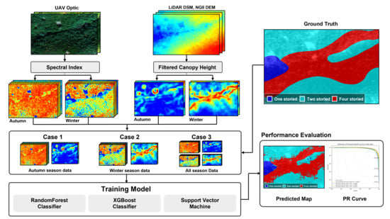
The study area covers a forest of about 0.02 km² on Samcheok-si, Gangwon-do, South Korea, which is a city with a coast to the east and the Taebaek mountain to the west. For the study, the forest vertical structure map was obtained from the field survey-based forest inventory plots. For the study, a forest vertical structure map was obtained, using a field survey. Figure 1 shows the RGB image and forest vertical structure maps of the study area. The study area consists of one-, two-, and four-storied forests. One-storied forests consist of a canopy and include Alnus japonica and Robinia pseudoacacia. The canopy layer in two-storied forests includes Pinus densiflora, Robinia pseudoacacia, and Platycarya, and the shrub layer includes Quercus serrata, Toxicodendron vernicifluum, Zanthoxylum piperitum, Rhododendron mucronulatum, and Quercus mongolica. Three-storied forests do not exist in the study area, but a four-storied forest is present, as shown in Figure 1. Four-storied forests consist of herbaceous, shrub, understory, and a canopy. The herbaceous layer includes Festuca ovina; the shrub layer includes Zanthoxylum piperitum, Rhododendron mucronulatum, and Toxicodendron vernicifluum; the understory includes Quercus serrata; and the canopy includes Pinus densiflora.

The data used in the study include two-seasonal optic images and LiDAR point clouds obtained by an optic sensor mounted on a UAV platform. The first UAV data were obtained on 22 October 2018 (fall), and the second UAV data were acquired on 29 November 2018 (winter). Temperatures were about 9.7 and 1.4 °C in the first and second acquisition times, respectively. Between the two acquisition dates, a deciduous period is included [19]. Deciduous trees have different characteristics before and after falling leaves. Of course, the acquisition date can be changed. For example, the winter data can be obtained in January or February. The reason why the November data are used is that the data used for forest applications are usually acquired during fall and winter season in South Korea.

The optical images were acquired using the RX02 camera that had five bands and was mounted on a UAV, including the blue, green, red, red edge, and near infrared band (NIR) (

Table 1. Band characteristics of optic images acquired by the RX02 camera mounted on a UAV.

Band	Center	Width
Blue	475 nm	32 nm
Green	560 nm	27 nm
Red	668 nm	16 nm
Red Edge	717 nm	12 nm
Near infrared	842 nm	57 nm

). The UAV flight height was about 200 m; the lateral and longitudinal overlaps were about 80%; and the scanning time was approximately 46 min. The image obtained using the UAV was acquired at a low altitude and has a high spatial resolution. The acquired optic images were processed with geometric correction through automatic aerial triangulation. Their spatial resolution was approximately 21–22 cm, and the orthorectified image was resampled to 20 cm, using bicubic interpolation. Optic images are advantageous in that the red edge band can be used. The red edge is normally used to monitor forest conditions. The UAV LiDAR data were obtained using the Velodyne LiDAR Puck (VLP-16) having an accuracy of 3 cm, and a two-seasonal DSM was generated by processing the LiDAR point clouds. The spatial resolution of the DSM was approximately 2 cm, and it was resampled to 20 cm. We attempted to create the DTM data from the point clouds, but the created DTM was not adequately accurate for this study because the forest was dense. Thus, DTM data created by the National Geographic Information Institute (NGII) were used for this study. The DTM data were resampled to 20 cm from 5 m. The NGII DTM is numerical topographic data generated through contour lines. The terrain height can be generally approximated with a smooth surface, and hence, re-sampling to 20 cm does not significantly affect model performance.

3. Methodology

For the feasibility test on the effectiveness of the multi-seasonal data, the UAV optic and LiDAR data were divided into three cases: (1) fall optic and LiDAR data (hereafter Case 1); (2) winter optic and LiDAR data (hereafter Case 2); and (3) fall and winter optic and LiDAR data (hereafter Case 3). The comparison between Case 1 and Case 2 allows us to analyze which seasonal data can increase model prediction accuracy. From case 3, it is possible to analyze how much the model prediction accuracy increases when using data from two seasons. The detailed workflow of this study is shown in Figure 2. The workflow is composed of three main steps: (1) normalized input data generation; (2) classification using the RF, XGBoost, and SVM models for Cases 1, 2, and 3; and (3) performance evaluation. In the first step, four spectral index maps, including the NDVI, GNDVI, NDRE, and SIPI indices, were created from a UAV optic image; the median and standard deviation maps of canopy heights were generated, using the UAV LiDAR-derived DSM, and the maps were then normalized by min–max scaling. In the second step, the training and test data were randomly selected from the normalized maps as 1% and 20% of the total pixels, respectively. Thus, the number of training data was 5320, and the number of test data was 106,400. The training and test data were selected so that they do not overlap in the entire study area. Subsequently, the training data were applied to the RF, XGBoost, and SVM models. In the last step, the performance of the three models was estimated from the test data, using the F1 score, which were then calculated.

3.1. Generation of the Normalized Input Data

3.1.1. Spectral Index Maps

Spectral index maps are widely used to analyze the characteristics of the Earth’s ecosystem by utilizing the spectral image characteristics, such as the vegetation and water resources [20]. They are also used to mitigate optical image distortions, including the topographic distortion and shadow effect. These distortions act as errors in quantitatively assessing and analyzing the indicators [21]. Thus, the spectral index mapping, which can be calculated by the pixel-based band ratio, is widely used to mitigate topographic distortion and the shadow effect [22]. To strengthen the vegetation analysis, four spectral indices, NDVI, GNDVI, NDRE, and SIPI, were selected and calculated from the UAV visible, red edge, and NIR images using the DN (digital number) values.

Table 2. Spectral indices used in this study.

Name	Acronyms	Equation
Normal Difference Vegetation Index	NDVI	$NDVI=\frac{NIR-RED}{NIR+RED}$
Green Normalized Difference Vegetation Index	GNDVI	$GNDVI=\frac{NIR-GREEN}{NIR+GREEN }$
Normalized Difference Red Edge Index	NDRE	$NDRE=\frac{NIR-RED Edge}{NIR+RED Edge}$
Structure Insensitive Pigment Index	SIPI	$SIPI=\frac{NIR-BLUE}{NIR-RED}$

presents the formulas of the four spectral indices used in this study.

NDVI is used to determine the vitality and density of vegetation, using the red and NIR band images. A high NDVI value indicates a high vitality and density of vegetation [23]. GNDVI uses green band images instead of red band images in the NDVI equation, which indicates the sensitivity of the vegetation to chlorophyll changes [24]. NDRE was used as an indicator of the health and vitality of vegetation [25]. The difference between the NDRE and NDVI indices is the difference in wavelength bands. The NDRE index was calculated using the red edge band, whereas the NIR index was estimated from the red band. Red edge bands are known to be more sensitive than red to changes in the health and vitality of vegetation. SIPI is used to analyze vegetation composed of multiple layers and is obtained using the blue, red, and NIR band images (see Table 2). The SIPI index can be used to estimate the ratio of carotenoid pigments in vegetation to determine the stress of vegetation [26]. The NDVI, GNDVI, NDRE, and SIPI index maps were normalized using the min–max scaling approach; hence, the pixel values of the index maps ranged from 0 to 1. Min–max scaling makes the minimum value to 0 and maximum value to 1. This is used to ensure that every feature has equal significance during training [27].

3.1.2. Canopy Height Maps

In this study, we created canopy height maps, using the UAV-derived DSM and NGII DTM. As aforementioned, the NGII DTM was obtained from contour lines by NGII, and the UAV-derived DSM was created by filtering LiDAR point clouds into the grid. The DSM data represent the surface height, including all the trees or artifacts on the Earth’s surface, whereas the DTM data indicate a terrain height excluding them. Thus, subtracting the DTM height from the DSM height can yield the height of the trees or artifacts. In this study, canopy height maps were produced by subtracting the NGII DTM from the UAV-derived DSM. The canopy height maps have a rough surface. This is because the UAV-derived DSM had a spatial resolution of 20 cm. To statistically present the rough surface, the median and standard deviation maps were extracted from the canopy height maps, using a moving kernel of 51 × 51. The kernel size was determined in consideration of the area (10 m × 10 m) used to classify the forest vertical structure. Therefore, the kernel size was determined by considering the average tree size in the study area. The median canopy height maps represent the central tendency of the canopy heights in the window kernel, whereas the standard deviation height maps show the amount of canopy height dispersion in the window kernel. Thus, the standard deviation will be large if the canopy height is diverse. More details on the median and standard deviation canopy height maps can be found in [28]. The median and standard deviation canopy height maps were normalized using the min–max scaling approach. The maps had pixel values ranging from 0 to 1.

3.2. Classification with Machine Learning Techniques

To classify the forest vertical structure in the study area, we applied three machine learning methods to the normalized NDVI, GNDVI, NDRE, and SIPI index maps. The machine learning methods used in this study were RF, XGBoost, and SVM. These three algorithms perform well in classifying images [29,30,31]. RF, XGBoost, and SVM are representative algorithms based on ensemble bagging, ensemble boosting, and kernel, respectively, and are used to determine which machine learning algorithms are effective for forest structure classification. More details are provided in the following sections.

3.2.1. Random Forest

RF is a machine learning technique proposed by [32]. He introduced the concepts of decision tree and bagging to train a machine learning model, using bootstrap aggregating (bagging) of the ensemble technique. This mitigated the overfitting problem in the decision tree [33]. The RF method randomly duplicates the learning data through bagging and trains multiple decision trees through the samples. It collects results, finds optimal characteristics, and predicts the classification results. Employing this ensemble method ensures better performance, compared to a single decision tree. Thus, the advantage of the RF method is that errors can be ignored, even if overfitting or underfitting decision trees are present.

3.2.2. XGBoost

XGBoost uses decision tree–based ensemble techniques, and it complements the drawbacks of the gradient boosting model [34]. The gradient boosting model gradually increases the model performance by assigning weight through the gradient descent approach. Although the gradient boost method has a good performance, overfitting problems may occur, as it does not include slow performance time and overfitting regulatory factors. Therefore, XGBoost was proposed to compensate for the drawbacks of the gradient boosting method. The XGBoost method enables data processing in parallel and further improves the performance of the model by including regulatory factors to prevent overfitting.

3.2.3. Support Vector Machine

The SVM method defines the criteria for classifying groups of samples, using a given learning model. This method was proposed by [35]. The SVM assumes that the learning data are within a vector space. The goals of this model are (1) to obtain a support vector to classify the data into groups and (2) calculate the optimal decision boundary [36]. In the SVM method, the support vector data are close to the decision boundary, and the margin represents the distance between the decision boundary and support vector. The optimal decision boundary maximizes the margin. SVM allows us (1) to classify data through simple linear separation and (2) to classify nonlinear data by identifying a decision boundary that can artificially increase the dimension of data using a kernel function, even in the case of nonlinear data without linear classification.

The three machine learning methods were applied to the three cases. As mentioned above, 1% of the total pixels were used for the training, whereas 20% of the total pixels were used for the test (performance evaluation). Hyperparameters used in each machine learning method were determined, using a random search cross-validation method to determine the best performance hyperparameter value through a combination of random variables within a certain range [37].

3.3. Performance Evaluation

The performance of the trained model was evaluated by calculating the precision, recall, precision–recall (PR) curve, false alarm rate (FAR), and F1 score. The precision is the fraction of the actual true pixels among those classified as true by the trained model, while recall is the fraction of the actual true pixels retrieved by the trained model. The PR curve is a graph that shows the change in precision and recall values with respect to the parameter adjustment of the algorithm. The PR curve has an average precision (AP) value as an indicator of the model classification performance, which was calculated using the area of the bottom line of the graph. Higher AP values indicate better model performance. Precision and recall are defined as follows [38]:

$$Precision=\frac{True Positive}{True Positive+False Positive}$$

(1)

$$Recall=\frac{True Positive}{True Positive+False Negative}$$

(2)

FAR is an incorrect detection rate, and the F1 score is used as an indicator to evaluate the model performance more exactly than the accuracy value when the number of labels is unbalanced. FAR and F1 score are defined as follows [39]:

$$FAR=1-Precision$$

(3)

$$F1 score=2\ast \frac{Precision\ast Recall}{Precision+Recall}$$

(4)

4. Results and Discussion

Figure 3 shows the true and false color composite images, LiDAR DSM, and NGII DTM. The true-color composite images shown in Figure 3a,d are displayed using red, green, and blue band images acquired on 22 October 2018 and 29 November 2018, respectively. The false-color composite images shown in Figure 3b,e are displayed, using red edge, NIR, and blue band images acquired on 22 October 2018 and 29 November 2018, respectively. In comparison with the images taken in October, those taken in November are relatively darker. Figure 3d,e is better identified for one-storied regions than Figure 3a,b. This is because one-storied structures are more sensitive to seasonal changes than two- and four-storied structures. Additionally, in the box of Figure 3c,f, the value of Figure 3f is smaller than that of Figure 3c. This change is caused by the decline in the height of trees as the leaves fall when the seasons change. Additionally, it is difficult to see a clear difference between the two- and four-storied regions in the true-color composite and false-color composite images.

Figure 4 shows the normalized NDVI, GNDVI, NDRE, and SIPI index maps, and the standard deviation and median canopy height maps calculated using the min–max normalization approach acquired on 22 October 2018. We normalized the pixel values within the 0 to 1 range through the min–max normalization to ignore the range and unit of the pixel values. The machine learning algorithms find patterns by analyzing and comparing features among different data. Thus, significant differences in the range and unit of feature for each data may prevent the model from being properly trained [40]. Thus, to avoid this problem and improve the model performance, the index and canopy height maps were normalized. The topographic effect of Figure 3a,b cannot be found in the normalized index maps shown in Figure 4a–d. This is why the index maps were selected instead of the original band images as the input data for the machine learning models. The brightness value of the optical image represents the reflectivity of the forest canopy, and it is difficult to find clear differences between one-, two-, and four-storied forests from Figure 4a–d. However, among the index maps of Figure 4a–d, the NDRE index map of Figure 4c describes the forest vertical structure relatively well. As seen in Figure 4e,f, the LiDAR-derived canopy height maps are correlated to classify the forest vertical structure. Nevertheless, because the canopy height map represents only the canopy height, there may be a clear limit in describing the vertical structure of the forest.

Figure 5 shows the normalized NDVI, GNDVI, NDRE, and SIPI index maps, and standard deviation and median canopy height maps acquired on 29 November 2018. The index maps of Figure 5a–d are significantly different, as they were obtained during different seasons, compared to those of Figure 4a–d. The leaves of the broadleaf trees fell, thereby decreasing the index values in Figure 4a–d. If the index values of Figure 5a–d are lower than those of Figure 4a–d, it is because of the distribution of broadleaf trees in the area. The winter index maps have a clearer difference between one-, two-, and four-storied forests than the fall index maps. We can find the same pattern in the LiDAR-derived canopy height maps. Moreover, the four-storied forest have higher values in the standard deviation canopy height maps, as seen in Figure 5e. This implies that a variety of trees exist in the four-storied forest. Additionally, the topographic effect in the winter index maps is slightly more severe than that the fall index maps. This is due to the different changes in tree conditions with respect to the terrain slope and aspect.

As mentioned above, the fall index and canopy height maps of Figure 4 were used as input data for Case 1, the winter index and canopy height maps of Figure 5 were used as input data for Case 2, and all the fall and winter maps were used as input data for Case 3. Machine learning methods, including RF, XGBoost, and SVM, were applied to the input data to classify the forest vertical structure. To determine the optimal hyperparameters for each model, we applied a randomized search cross-validation approach to each model and case. The randomized search cross-validation approach conducts the cross-verification of randomly selected variables over a specified range of values. This method finds variables that provide the best performance in a given model [37].

Table 3. Hyperparameters used for the RF, XGBoost, and SVM models.

Model	Hyperparameter	Value
		Case 1	Case 2	Case 3
RF	max_depth	962	137	979
	n_estimators	319	465	292
XGBoost	learning_rate	0.13	0.39	0.10
	max_depth	581	139	765
	n_estimators	438	463	583
SVM	C	8506	5517	7030
	gamma	0.97	0.86	0.90
	kernel	rbf	rbf	rbf

presents the optimal hyperparameters determined by the method for the three models in Cases 1, 2, and 3. As presented in Table 3, the hyperparameters used were (1) the maximum depth of the tree and the number of decision trees in the RF model, (2) the learning rate, tree depth, and number of decision trees in XGBoost, and (3) error allowance, flexibility to draw decision boundaries, and kernel function in SVM.

Using the determined optimal hyperparameters, the RF, XGBoost, and SVM models were run by applying the input data for Cases 1, 2, and 3. Figure 6 shows the classification maps estimated from RF, XGBoost, and SVM in three cases. The classification results from the RF model for Cases 1, 2, and 3 are shown in Figure 6a–c; the XGBoost model is represented in Figure 6d–f; the SVM model is shown in Figure 6g–i. The results of the SVM model for Cases 1, 2, and 3 are shown in Figure 6g–i, respectively. Through the visual analysis of Figure 6, some of the results are summarized as follows. First, for all the three models, the classification results for Case 1 are considerably worse than those of Cases 2 and 3. This is because it was difficult to find the clear differences between one-, two-, and four-storied forests from the fall index maps and LiDAR-derived maps (see Figure 4). Second, the classification performance in Case 3 is higher than that in Case 2. We identified a synergy effect through two-seasonal data in the forest vertical structure classification. Third, in all the cases, the classification performances of the RF, XGBoost, and SVM models are not significantly different. The performance difference between the three models is lower than that resulting from the input data. This implies that the data used are more important than the model used.

The significant difference between Cases 1, 2, and 3 can be found in boxes A and B, as shown in Figure 6. The significant difference in box A is as follows: (1) In Case 1, the boundaries between the one-, two-, and four-storied forests were not clear, and the one- and two-storied forests were classified as four-storied forests in some areas. (2) The classification results from Case 2 show that the classification of the one-storied forest was considerably better than that of Case 1, and the boundary between the two- and four-storied forests became clearer than that of Case 1. (3) In Case 3, the one-storied forest identification and the boundary between the two- and four-storied forests became almost perfect. Moreover, the identification of the one-storied forest significantly improved from Cases 1 to 3, in box B.

Figure 7 shows the PR curve graphs estimated from the classification results of the RF, XGBoost, and SVM models for Cases 1, 2, and 3. The yellow lines show the microaverage PR curves, and the blue, orange, and green lines represent those for the one-, two-, and four-storied forests, respectively. In all cases, the curves of RF and XGBoost are similar, whereas the SVM shows different curves. Moreover, the SVM curves are not smooth but considerably distorted, as shown in Figure 7g–i. This indicates that the SVM model has a lower classification performance. In most cases, the classification performance of the two-storied forest is the highest, whereas that of the one-storied forest is the lowest. There is almost no difference between the classification performance of one- and two-storied forests in Case 3, whereas this is very large in Case 1 because the two-storied forest is dominant in the study area, while the one-storied forest is distributed only in small areas.

As shown in Figure 7a–c, the AP values estimated by the RF model are approximately 0.85, 0.94, and 0.97 for Cases 1, 2, and 3, respectively. The classification performance of Case 3 is approximately 0.12 and 0.03 times better than Cases 1 and 2, respectively. The AP values of the XGBoost model are approximately 0.86, 0.95, and 0.98 for Cases 1, 2, and 3, respectively. The AP values of the XGBoost model are similar to those of the RF model. The XGBoost model is slightly superior to the RF model. In the XGBoost model, the classification performance of Case 3 is the best, and that of the one-storied forest is the worst in Case 1. The AP values of the SVM model are approximately 0.78, 0.84, and 0.92 for Cases 1, 2, and 3, respectively. The SVM AP values are worse than those of the other models. Especially for Case 2, the SVM AP values are approximately 0.10 to 0.11 lower than those of the RF and XGBoost models. In other words, based on the AP values, XGBoost shows the best classification performance, that of RF is similar to XGBoost, and SVM shows the worst performance.

Table 4. Precision, recall, FAR, and F1 score based on the results from the RF, XGBoost, and SVM models.

Model	Case	Evaluation Metrics	One-Storied	Two-Storied	Four-Storied	Macro Average
RF	Case 1	Precision	0.76	0.78	0.73	0.76
		Recall	0.28	0.82	0.74	0.61
		False Alarm Rate	0.24	0.22	0.27	0.24
		F1 score	0.41	0.80	0.74	0.65
	Case 2	Precision	0.82	0.89	0.84	0.85
		Recall	0.63	0.87	0.87	0.79
		False Alarm Rate	0.18	0.11	0.16	0.15
		F1 score	0.71	0.88	0.85	0.81
	Case 3	Precision	0.94	0.93	0.88	0.92
		Recall	0.81	0.92	0.91	0.88
		False Alarm Rate	0.06	0.07	0.12	0.08
		F1 score	0.87	0.92	0.90	0.90
XGBoost	Case 1	Precision	0.68	0.79	0.73	0.73
		Recall	0.40	0.81	0.75	0.65
		False Alarm Rate	0.32	0.21	0.27	0.27
		F1 score	0.50	0.80	0.74	0.68
	Case 2	Precision	0.79	0.89	0.84	0.84
		Recall	0.69	0.87	0.88	0.81
		False Alarm Rate	0.21	0.11	0.16	0.16
		F1 score	0.74	0.88	0.86	0.83
	Case 3	Precision	0.94	0.94	0.91	0.93
		Recall	0.90	0.93	0.92	0.92
		False Alarm Rate	0.06	0.06	0.09	0.07
		F1 score	0.92	0.94	0.92	0.92
SVM	Case 1	Precision	0.62	0.76	0.71	0.70
		Recall	0.29	0.80	0.71	0.60
		False Alarm Rate	0.38	0.24	0.29	0.30
		F1 score	0.40	0.78	0.71	0.63
	Case 2	Precision	0.68	0.88	0.81	0.79
		Recall	0.69	0.84	0.86	0.79
		False Alarm Rate	0.32	0.12	0.19	0.21
		F1 score	0.68	0.85	0.83	0.79
	Case 3	Precision	0.85	0.92	0.89	0.88
		Recall	0.92	0.91	0.89	0.91
		False Alarm Rate	0.15	0.08	0.11	0.12
		F1 score	0.88	0.91	0.89	0.90

shows precision, recall, FAR, and F1 score for each model and case in this study. Initially, in Case 1, the RF model is the best in terms of precision and FAR, whereas the XGBoost model is the best in terms of recall and F1 score. The RF and XGBoost models are better than the SVM model, and the best performing model is the XGBoost model; however, the performance difference between them is not large (see Table 1). Secondly, Case 2 has the same pattern as the Case 1 results; the best performing model is the XGBoost model, and the performance difference between the models is not large. However, the performance difference between Cases 1 and 2 is as large as ~0.16 in terms of the F1 score. Last, in Case 3, the XGBoost model performs best in all evaluation parameters, including the precision, recall, FAR, and F1 score. The classification performance of Case 3 in terms of the F1 score is improved by ~0.1 compared to Case 2 and by ~0.26 compared to Case 1. From the results, we can conclude that (1) XGBoost is the best model among the RF, XGBoost and SVM models; (2) two-seasonal input data have better performance than one-seasonal input data in the machine learning techniques; (3) winter season input data are better than the fall season input data for the forest vertical structure mapping using the RF, XGBoost, and SVM models; (4) the performance difference between the models is not significant, whereas the difference between the input data cases is very large; and (5) the classification performance based on the F1 score is as high as 0.92 when the XGBoost model is applied to the two-seasonal input data. In previous studies, Kwon et al. [41] had about 0.662 classification accuracy and Lee et al. [42] showed approximately 0.657. It means that our results have remarkably improved, compared to previous studies. In addiion, this result shows that forest vertical structure maps can be generated with accuracy greater than 0.9 when the XGBoost method is applied to multi-seasonal high-resolution optic and LiDAR data.

5. Conclusions

Forest vertical structure mapping using machine learning algorithms—RF, XGBoost, and SVM models—was investigated in this study. Several studies have conducted feasibility tests for classifying the forest vertical structure, using remote-sensed data and machine learning techniques, but the classification performance was lower than 0.8. They did not analyze the effectiveness of the multi-seasonal data and that of the high-resolution UAV LiDAR data in the forest vertical structure classification.

In this study, we investigated the effectiveness of multi-seasonal data and high-resolution LiDAR data acquired from a UAV platform in the forest vertical structure classification, using the RF, XGBoost, and SVM models. To apply the optical images and LiDAR data to the machine learning methods, the NDVI, GNDVI, NDRE, and SIPI index maps were generated, and the median and standard deviation canopy height maps were created. The spectral index maps, and the median and standard deviation canopy height maps were used as the input data for the three models. Moreover, to test the multi-seasonal effectiveness, the input data were divided into three cases: (1) using fall optic and LiDAR data, (2) using winter-optic and LiDAR data, and (3) using fall and winter optic and LiDAR data. Finally, the performance of the forest vertical structure classification was evaluated and compared among the accuracies calculated from the three cases.

In all cases, the PR curves of the RF and XGBoost models were very similar but differed from those of the SVM model. The SVM curves were considerably distorted rather than smooth. The AP values from the RF, XGBoost, and SVM models, respectively, were approximately as follows for Cases 1, 2 and 3, respectively: 0.85, 0.86, and 0.78; 0.94, 0.95, and 0.84; and 0.97, 0.98, and 0.92. The performance of the XGBoost model was the best, but that of the RF model was comparable. The SVM model was worse than the other models. The precision, recall, FAR, and F1 score from the RF, XGBoost, and SVM models were calculated for Cases 1, 2, and 3. In Cases 1 and 2, the RF model performed best in terms of the precision and FAR, whereas the XGBoost model performed best in terms of the recall and F1 score. In Case 3, the XGBoost model performed best in all evaluation parameters, and the F1 score in this case reached 0.92. The results show that the XGBoost method enables us to create vertical forest structure maps with an accuracy greater than 0.9 if multi-seasonal high-resolution optic and LiDAR data are used. This implies that forest vertical structure maps can be produced by using machine learning techniques and high-resolution UAV optic and LiDAR data instead of field surveys.

However, this study has a limitation. Since RF, XGBoost, and SVM are pixel-based models, they cannot be learned by applying spatial characteristics. Therefore, further study should be conducted, using the patch-based model, and performance comparisons between the patch-based model and the current model should be performed.

References

1. Prasad, R.; Kant, S. Institutions, Forest Management, and Sustainable Human Development: Experience from India. Environ. Dev. Sustain. 2003, 5, 353–367. [Google Scholar] [CrossRef]
2. Kibria, A.S.; Behie, A.; Costanza, R.; Groves, C.; Farrell, T. The value of ecosystem services obtained from the protected forest of Cambodia: The case of Veun Sai-Siem Pang National Park. Ecosyst. Serv. 2017, 26, 27–36. [Google Scholar] [CrossRef]
3. Lee, S.; Lee, S.; Lee, M.-J.; Jung, H.-S. Spatial Assessment of Urban Flood Susceptibility Using Data Mining and Geographic Information System (GIS) Tools. Sustainability 2018, 10, 648. [Google Scholar] [CrossRef] [Green Version]
4. Bohn, F.J.; Huth, A. The importance of forest structure to biodiversity–productivity relationships. R. Soc. Open Sci. 2017, 4, 160521. [Google Scholar] [CrossRef] [Green Version]
5. Kimes, D.; Ranson, K.; Sun, G.; Blair, J. Predicting lidar measured forest vertical structure from multi-angle spectral data. Remote Sens. Environ. 2006, 100, 503–511. [Google Scholar] [CrossRef]
6. Froidevaux, J.; Zellweger, F.; Bollmann, K.; Jones, G.; Obrist, M.K. From field surveys to LiDAR: Shining a light on how bats respond to forest structure. Remote Sens. Environ. 2016, 175, 242–250. [Google Scholar] [CrossRef] [Green Version]
7. Lee, Y.-S.; Baek, W.-K.; Jung, H.-S. Forest vertical Structure classification in Gongju city, Korea from optic and RADAR satellite images using artificial neural network. Korean J. Remote Sens. 2019, 35, 447–455. [Google Scholar]
8. Zimble, D.A.; Evans, D.L.; Carlson, G.C.; Parker, R.C.; Grado, S.C.; Gerard, P.D. Characterizing vertical forest structure using small-footprint airborne LiDAR. Remote Sens. Environ. 2003, 87, 171–182. [Google Scholar] [CrossRef] [Green Version]
9. Hyde, P.; Dubayah, R.; Walker, W.; Blair, J.B.; Hofton, M.; Hunsaker, C. Mapping forest structure for wildlife habitat analysis using multi-sensor (LiDAR, SAR/InSAR, ETM+, Quickbird) synergy. Remote Sens. Environ. 2006, 102, 63–73. [Google Scholar] [CrossRef]
10. Navalgund, R.R.; Jayaraman, V.; Roy, P.S. Remote sensing applications: An overview. Curr. Sci. 2007, 93, 1747–1766. [Google Scholar]
11. Campbell, J.B.; Wynne, R.H. Introduction to Remote Sensing; Guilford Press: New York, NY, USA, 2011. [Google Scholar]
12. Camps-Valls, G. Machine Learning in Remote Sensing Data Processing. In Proceedings of the 2009 IEEE International Workshop on Machine Learning for Signal Processing, Grenoble, France, 1–4 September 2009. [Google Scholar]
13. Bermant, P.C.; Bronstein, M.M.; Wood, R.J.; Gero, S.; Gruber, D.F. Deep Machine Learning Techniques for the Detection and Classification of Sperm Whale Bioacoustics. Sci. Rep. 2019, 9, 12588. [Google Scholar] [CrossRef] [Green Version]
14. Batista, G.; Monard, M.C. An analysis of four missing data treatment methods for supervised learning. Appl. Artif. Intell. 2003, 17, 519–533. [Google Scholar] [CrossRef]
15. Breck, E.; Polyzotis, N.; Roy, S.; Whang, S.; Zinkevich, M. Data Validation for Machine Learning. In Proceedings of the MLSys 2019, Stanford, CA, USA, 31 March–2 April 2019. [Google Scholar]
16. Gudivada, V.; Apon, A.; Ding, J. Data quality considerations for big data and machine learning: Going beyond data cleaning and transformations. Int. J. Adv. Softw. 2017, 10, 1–20. [Google Scholar]
17. Miller, J.R.; White, H.P.; Chen, J.M.; Peddle, D.R.; McDermid, G.; Fournier, R.A.; Shepherd, P.; Rubinstein, I.; Freemantle, J.; Soffer, R.; et al. Seasonal change in understory reflectance of boreal forests and influence on canopy vegetation indices. J. Geophys. Res. Space Phys. 1997, 102, 29475–29482. [Google Scholar] [CrossRef]
18. Potter, B.E.; Teclaw, R.M.; Zasada, J.C. The impact of forest structure on near-ground temperatures during two years of contrasting temperature extremes. Agric. For. Meteorol. 2001, 106, 331–336. [Google Scholar] [CrossRef]
19. Kim, J.H. Seasonal Changes in Plants in Temperate Forests in Korea. Ph.D. Thesis, The Seoul National University, Seoul, Korea, 2019. [Google Scholar]
20. Motohka, T.; Nasahara, K.; Murakami, K.; Nagai, S. Evaluation of Sub-Pixel Cloud Noises on MODIS Daily Spectral Indices Based on in situ Measurements. Remote Sens. 2011, 3, 1644–1662. [Google Scholar] [CrossRef] [Green Version]
21. Soenen, S.; Peddle, D.; Coburn, C. SCS+C: A modified Sun-canopy-sensor topographic correction in forested terrain. IEEE Trans. Geosci. Remote Sens. 2005, 43, 2148–2159. [Google Scholar] [CrossRef]
22. Van Beek, J.; Tits, L.; Somers, B.; Deckers, T.; Janssens, P.; Coppin, P. Reducing background effects in orchards through spectral vegetation index correction. Int. J. Appl. Earth Obs. Geoinf. 2015, 34, 167–177. [Google Scholar] [CrossRef]
23. Ghazal, M.; Al Khalil, Y.; Hajjdiab, H. UAV-based remote sensing for vegetation cover estimation using NDVI imagery and level sets method. In Proceedings of the 2015 IEEE ISSPIT, Abu Dhabi, United Arab Emirates, 7–10 December 2015. [Google Scholar] [CrossRef]
24. Wahab, I.; Hall, O.; Jirström, M. Remote Sensing of Yields: Application of UAV Imagery-Derived NDVI for Estimating Maize Vigor and Yields in Complex Farming Systems in Sub-Saharan Africa. Drones 2018, 2, 28. [Google Scholar] [CrossRef] [Green Version]
25. Jorge, J.; Vallbé, M.; Soler, J.A. Detection of irrigation inhomogeneities in an olive grove using the NDRE vegetation index obtained from UAV images. Eur. J. Remote Sens. 2019, 52, 169–177. [Google Scholar] [CrossRef] [Green Version]
26. Zhang, N.; Su, X.; Zhang, X.; Yao, X.; Cheng, T.; Zhu, Y.; Cao, W.; Tian, Y. Monitoring daily variation of leaf layer photosynthesis in rice using UAV-based multi-spectral imagery and a light response curve model. Agric. For. Meteorol. 2020, 291, 108098. [Google Scholar] [CrossRef]
27. Khan, R.S.; Bhuiyan, M.A.E. Artificial Intelligence-Based Techniques for Rainfall Estimation Integrating Multisource Precipitation Datasets. Atmosphere 2021, 12, 1239. [Google Scholar] [CrossRef]
28. Kwon, S.-K.; Jung, H.-S.; Baek, W.-K.; Kim, D. Classification of Forest Vertical Structure in South Korea from Aerial Orthophoto and Lidar Data Using an Artificial Neural Network. Appl. Sci. 2017, 7, 1046. [Google Scholar] [CrossRef] [Green Version]
29. Chandra, M.A.; Bedi, S.S. Survey on SVM and their application in image classification. Int. J. Inf. Technol. 2018, 13, 1–11. [Google Scholar] [CrossRef]
30. Horning, N. Random Forests: An algorithm for image classification and generation of continuous fields data sets. In Proceedings of the International Conference on Geoinformatics for Spatial Infrastructure Development in Earth and Allied Sciences, Osaka, Japan, 9–11 December 2010; Volume 911. [Google Scholar]
31. Memon, N.; Patel, S.B.; Patel, D.P. Comparative Analysis of Artificial Neural Network and XGBoost Algorithm for PolSAR Image Classification. In Lecture Notes in Computer Science; Springer International Publishing: Berlin/Heidelberg, Germany, 2019; pp. 452–460. [Google Scholar] [CrossRef]
32. Breiman, L. Random forests. Mach. Learn. 2001, 45, 5–32. [Google Scholar] [CrossRef] [Green Version]
33. Lee, S.; Kim, J.-C.; Jung, H.-S.; Lee, M.J.; Lee, S. Spatial prediction of flood susceptibility using random-forest and boosted-tree models in Seoul metropolitan city, Korea. Geomat. Nat. Hazards Risk 2017, 8, 1185–1203. [Google Scholar] [CrossRef] [Green Version]
34. Joharestani, M.Z.; Cao, C.; Ni, X.; Bashir, B.; Talebiesfandarani, S. PM2.5 Prediction Based on Random Forest, XGBoost, and Deep Learning Using Multisource Remote Sensing Data. Atmosphere 2019, 10, 373. [Google Scholar] [CrossRef] [Green Version]
35. Cortes, C.; Vapnik, V. Support-Vector Networks. Mach. Learn. 1995, 20, 273–297. [Google Scholar] [CrossRef]
36. Hwang, J.-I.; Jung, H.-S. Automatic Ship Detection Using the Artificial Neural Network and Support Vector Machine from X-Band Sar Satellite Images. Remote Sens. 2018, 10, 1799. [Google Scholar] [CrossRef] [Green Version]
37. Bergstra, J.; Bengio, Y. Random search for hyper-parameter optimization. J. Mach. Learn. Res. 2012, 13, 281–305. [Google Scholar]
38. Buckland, M.; Gey, F. The relationship between recall and precision. J. Am. Soc. Inf. Sci. 1994, 45, 12–19. [Google Scholar] [CrossRef]
39. Chicco, D.; Jurman, G. The advantages of the Matthews correlation coefficient (MCC) over F1 score and accuracy in binary classification evaluation. BMC Genom. 2020, 21, 6. [Google Scholar] [CrossRef] [PubMed] [Green Version]
40. Jo, J.-M. Effectiveness of Normalization Pre-Processing of Big Data to the Machine Learning Performance. J. Inf. Commun. Converg. Eng. 2019, 14, 547–552. [Google Scholar]
41. Kwon, S.-K.; Lee, Y.-S.; Kim, D.-S.; Jung, H.-S. Classification of Forest Vertical Structure Using Machine Learning Analysis. Korean J. Remote Sens. 2019, 35, 229–239. [Google Scholar]
42. Lee, Y.-S.; Lee, S.; Baek, W.-K.; Jung, H.-S.; Park, S.-H.; Lee, M.-J. Mapping Forest Vertical Structure in Jeju Island from Optical and Radar Satellite Images Using Artificial Neural Network. Remote Sens. 2020, 12, 797. [Google Scholar] [CrossRef] [Green Version]
Figure 1. (a) Study area and (b) forest vertical structure map (ground truth).
Remotesensing 13 04282 g001
Figure 2. Detailed workflow of this study.
Remotesensing 13 04282 g002
Figure 3. (a) True-color composite image (R,G,B), (b) false-color composite image (red edge, NIR, B), and (c) LiDAR DSM obtained on 22 October 2018; (d) true-color composite image (R,G,B), (e) false-color composite image (red edge, NIR, B), and (f) LiDAR DSM obtained on 29 November 2018; and (g) NGII DTM.
Remotesensing 13 04282 g003
Figure 4. (a) Normalized NDVI, (b) GNDVI, (c) NDRE, and (d) SIPI index maps; (e) normalized standard deviation and (f) median canopy height maps extracted from UAV-based optical and LiDAR data acquired on 22 August 2018.
Remotesensing 13 04282 g004
Figure 5. (a) Normalized NDVI, (b) GNDVI, (c) NDRE, and (d) SIPI index maps; (e) normalized standard deviation and (f) median canopy height maps extracted from UAV-based optical and LiDAR data acquired on 29 November 2018.
Remotesensing 13 04282 g005
Figure 6. Classification result of the forest vertical structure using (ac) the RF model in Cases 1, 2, and 3, respectively, (df) the XGBoost model in Cases 1, 2, and 3, respectively, and (gi) the SVM model in Cases 1, 2, and 3, respectively. Box A represented the boundary of one-, two-, and four-storied, and Box B represented the center of one-storied.
Remotesensing 13 04282 g006
Figure 7. Precision–recall curves from (ac) the RF model in Cases 1, 2, and 3, respectively; (df) the XGBoost model in Cases 1, 2, and 3, respectively; and (gi) the SVM model in Cases 1, 2, and 3, respectively. Classes 0, 1, and 2 indicate one-, two-, and four-storied forests, respectively.
Remotesensing 13 04282 g007