
A Lightweight Detection Model for SAR Aircraft in a Complex Environment


1
School of Electronics and Communication Engineering, Shenzhen Campus, Sun Yat-sen University, Shenzhen 518107, China
2
College of Electronic Science, National University of Defense Technology, Changsha 410073, China
*
Author to whom correspondence should be addressed.
Remote Sens. 2021, 13(24), 5020; https://doi.org/10.3390/rs13245020
Submission received: 14 November 2021
/
Revised: 6 December 2021
/
Accepted: 7 December 2021
/
Published: 10 December 2021
(This article belongs to the Special Issue Advances in Geospatial Object Detection and Tracking Using AI)
Abstract
:Recently, deep learning has been widely used in synthetic aperture radar (SAR) aircraft detection. However, the complex environment of the airport—consider the boarding bridges, for instance—greatly interferes with aircraft detection. Besides, the detection speed is also an important indicator in practical applications. To alleviate these problems, we propose a lightweight detection model (LDM), mainly including a reuse block (RB) and an information correction block (ICB) based on the Yolov3 framework. The RB module helps the neural network extract rich aircraft features by aggregating multi-layer information. While the RB module brings more effective information, there is also redundant and useless information aggregated by the reuse block, which is harmful to detection precision. Therefore, to accurately extract more aircraft features, we propose an ICB module combining scattering mechanism characteristics by extracting the gray features and enhancing spatial information, which helps suppress interference in a complex environment and redundant information. Finally, we conducted a series of experiments on the SAR aircraft detection dataset (SAR-ADD). The average precision was 0.6954, which is superior to the precision values achieved by other methods. In addition, the average detection time of LDM was only 6.38 ms, making it much faster than other methods.
1. Introduction
Synthetic aperture radar (SAR) has all-weather and all-time characteristics, which lays the foundation for applications of agriculture and forestry monitoring, geological surveying and mapping, marine traffic supervision, and airport management. In the imaging process, as shown in Figure 1, SAR first launches a short pulse. After hitting the target, part of the energy returns and is received. Then, radar stores the historical Doppler phase of the target echo and generates the synthetic image, which is beneficial to improving the azimuth resolution. SAR imaging is also affected by sensor type, parameter settings, and observation direction. The scattering mechanism of SAR [1] can lead to large differences between images of the same target under different conditions. Therefore, aircraft detection is a challenging task for SAR images.
Traditional methods [2,3,4,5,6,7,8,9] have made some improvements in SAR image target detection, but those methods require prior information and lack robustness. Besides, the detection times of those algorithms also limits the practical application. SAR automatic target detection [9] generally includes detection, discrimination, and classification. The detection part mainly uses the constant false alarm rate (CFAR) algorithm [2,3] to extract features and determine candidate locations, including targets and false alarms. The discrimination part is mainly used to eliminate redundancy by using target likeness. The classification part weighs various target likeness scores and prior information to judge target classification. The detection part is the most important and is mainly based on CFAR. The CFAR algorithm sets the false alarm rate, models the pixels in the sliding window, estimates the detection threshold, and compares the pixel value with the detection threshold to judge whether it is the target pixel. It repeats this calculation process until all image pixels are visited. The basic CFAR detector [7] includes CA-CFAR, GO-CFAR, SO-CFAR, and OS-CFAR. CA-CFAR uses all pixels in the hollow window and averages to estimate the statistical parameters of the background clutter, which has better detection performance in the self region. OS-CFAR arranges the pixels in the window in ascending order, selects the kth number as noise, and then estimates the background clutter, which is good for detecting small targets. GO-CFAR can detect targets at the edge of clutter, but cannot distinguish two closely spaced targets. CFAR is based on background clutter estimation, and it does not consider the statistical characteristics of the target. GLRT [8] takes the statistical distribution of the target into account. In addition to the CFAR algorithm, wavelet analysis and empirical mode decomposition [10,11] are also used for SAR aircraft detection. Wavelet analysis is based on the pyramid decomposition model with many sub-images of different frequencies. Empirical mode decomposition also generates sub-images and focuses more on directional information. There is rich target information in the sub-images. However, in practical applications, the prior information of the target is unknown. Besides, the scattering characteristics of the clutter background are related to the specific environment. It is difficult to maintain excellent performance in different detection scenes.
In recent years, methods based on convolutional neural networks (CNN) have achieved better performance in optical image target detection. Deep learning target detection methods can be divided into one-stage methods [12,13,14,15] and two-stage methods [16,17]. A two-stage method generates target candidate regions and then predicts the positions and classes of possible targets. Differently, the one-stage method uses regression for target detection and directly predicts category and location. With the help of the candidate region extraction, the two-stage method has more accurate detection results but spends much more time making inferences than the one-stage method. Faster R-CNN [16] uses a region proposal network to generate regions of interest, and then get target classification and bounding box regression. Yolov3 [14] divides the input into S × S grids, and each grid predicts multiple bounding boxes. Yolov3 employs a feature pyramid structure and has good detection performance in multi-scale target detection. SSD [15] searches the best candidate box on multiple feature maps and directly predicts the classification and position, which fully integrates the advantages of Faster R-CNN and Yolo. With the vigorous development of deep learning, there are many excellent one-stage and two-stage methods for target detection in optical images.
Due to the excellent detection performance of deep learning with optical images, researchers apply those methods to SAR images. In [18], Wei et al. employed semi-supervised learning to alleviate the lack of target-level labeled samples and an attention module to focus on significant features while suppressing the clutter. Gong et al. [19] used a sparse autoencoder, CNN, and unsupervised clustering for joint interpretation of spatial-temporal SAR images. In [20], He et al. used a sparse autoencoder learning algorithm for aircraft classification. Wang et al. [21] used a salient feature algorithm to find the possible targets and adopted a CNN method to accurately detect targets from those candidates. He et al. [22] proposed a parallel network to detect an overall target and corresponding components, respectively, and take advantage of the maximum probability and prior information to suppress wrong targets. An et al. [23] optimized a target detection method with the rotated bounding boxes to locate the targets more accurately compared with horizontal bounding boxes, including a multi-layer prior generation strategy (to detect small target), a modified rotated box encoding scheme, and a focal loss method (to balance positive and negative samples). However, these above methods work using small regions that are manually selected in SAR images, which directly removes the interference around the aircraft targets. With much interference, those methods are difficult to apply. Therefore, a complex background environment is a challenge.
To expand the scope of applications, some methods start to detect aircraft in the approximate airport region. Luo et al. [24] proposed an efficient bidirection path aggregation attention network with the equipment of Yolov5s, the involution enhanced path aggregation module to extract important features, and the effective residual shuffle attention module to overcome the interference information. Zhang et al. [25] proposed a cascaded three-look network based on Faster R-CNN [16] to detect potential aircraft, and a region growing algorithm to extract the airfield runway accurately, which is used to filter out false alarms. Zhao et al. [26] made use of Yolov3 [14] to determine the approximate area of the airport, and extracted connected components of the airport region via Gaussian filtering algorithm to suppress wrong aircraft detection results. Guo et al. [27] extracted the airport area and proposed an algorithm that uses enhancing scattering information and deep learning. They used the Harris–Laplace detector to extract strong scattering points, clustered initial aircraft targets for image preprocessing, employed feature pyramid networks [28], and used a modified attention module to detect aircraft. Zhao et al. [29] proposed the pyramid attention dilated network mainly consisting of a multibranch dilated convolution module to enhance the discrete features of aircraft, and a convolution block attention module (CBAM) [30] to refine redundant information and highlight significant scattering information. Wang et al. [31] first detected the airport runaway area, and then proposed the efficient weighted feature fusion and attention network for reducing the interference and enhancing feature extraction, which is beneficial to accurately and effectively detecting aircraft.
The above methods have high detection accuracy in relatively simple background environments, such as runways or squares. However, many aircraft are parked in more complex environments, such as near the terminal buildings or boarding bridges, which usually leads to poor detection. In complex scenes, background noise adversely affects aircraft detection. The detection time is also an important indicator in practical applications. To rapidly detect aircraft targets in a relatively complex environment, we propose a lightweight detection model (LDM) which can use the information effectively and efficiently with the help of the reuse block (RB) and information correction block (ICB). Based on multi-layer information fusion, we propose the RB module, which helps to extract more aircraft features in a complex environment. Inspired by the characteristics of SAR image scattering features, especially gray-scale features, we propose the ICB module, which effectively suppresses redundant information and background interference. The contributions are as follows.
- (1)
- We propose a lightweight detection model to detect SAR aircraft targets in complex environments, and the proposed method achieves superior detection performance far more rapidly than other CNN methods.
- (2)
- We propose an RB module to acquire more aircraft features during feature extraction by aggregating multi-layer information.
- (3)
- We propose an ICB module to enhance effective aircraft features, and suppress redundant information from the RB module and interference from the complex environment by enhancing salient points, especially gray-scale features.
2. Materials and Methods
2.1. Overall Detection Framework
To rapidly detect aircraft targets, we require two key solutions. The first must extract more aircraft features. The second must obtain accurate aircraft features from complex scenes. Therefore, we propose an RB module to aggregate multi-layer information and an ICB module to enhance salient points. With the help of RB and ICB modules, a lightweight and high-speed detection model based on the Yolov3 framework [14] is proposed. We use Yolov3-tiny as the baseline, which is lightweight with few layers. In the structure, we use a stack of two RB modules and then an ICB module. As these two RB modules are on different resolution feature maps, it is beneficial to extract more features. After using the ICB module, we can extract more effective features and suppress interference.
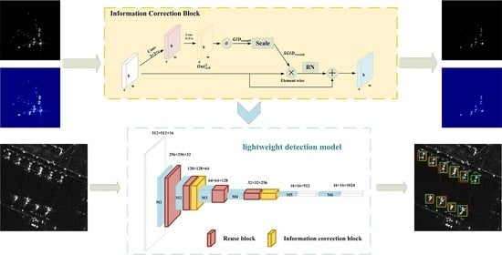
As shown in Figure 2, our lightweight detection model is composed of two parts. The detection part is shown in the dashed box, and the remainder is an extraction part. We label 6 max-pooling layers in Figure 2 as M1, M2, M3, M4, M5, and M6. The max-pooling layer is beneficial to data dimensionality reduction and detection model robustness. LDM includes 4 RB modules to employ more information, which replace the convolutional layer after M1, M2, M3, and M4 in the baseline. The ICB module is placed before M3 and M5 to accurately enhance aircraft features and suppress background interference. The output size after each layer is shown in Figure 2, such as 32 × 32 × 256, which, respectively, represent the height, width, and number of channels.
2.2. Reuse Block
2.2.1. Motivation
We hope to extract rich and effective aircraft features, but the input information or gradient information may vanish after passing several layers [32]. Huang et al.’s method [32] uses all previous layers as input, which helps to alleviate the loss of gradient information and make more effective use of features. However, dense connection causes heavy computational cost. For high speed, we propose the RB module with the simplified dense structure [32] to improve the utilization of aircraft features by aggregating multi-layer information.
2.2.2. The Structure of the Reuse Block
The full structure of the reuse block is shown in Figure 3. Specifically, we first increase the feature dimensions by using a 1 × 1 convolutional layer , which is the way to change the number of channels and synthesize the information along the channel direction. Then, we extract aircraft features with a stack of two 3 × 3 convolutional layers , which reduces the number of calculations required, yet acquires the same effective receptive field as 5 × 5 convolutional layers. After that, we aggregate features with the help of concatenation operation to reuse feature maps in the previous three layers. Finally, we extract features from the concatenated feature maps. The precise equations in the RB module are as follows:
where represents the input feature maps. The outputs of the three consecutive convolutional layers are , , and , respectively. is the concatenate operation. is the result of reusing information, and is the feature extracted from the reuse information result.
2.3. Information Correction Block
2.3.1. Motivation
In a complex environment, the background interferes greatly with target detection. The scattering characteristics are different for aircraft and background. Therefore, we use the unique characteristics of SAR images to assist the detection model with extracting more effective aircraft features. As shown in Figure 1, SAR image data include the reflection intensity of the target (regarding the radar beam) and phase information. In an SAR image, the point feature is the response to each resolution cell and is the most basic feature. Extracting aircraft features by salient points is an excellent method; these points are related to the maximum values of the scattering region and physical scattering centers [33]. This inspired us to enhance the salient points in the feature maps to assist the neural network with learning aircraft features.
2.3.2. Salient Point
Salient points are related to the pixel amplitude. In relation to that, we had a simple idea that enhances the pixels with high amplitudes and suppresses other pixels. For the calculation process shown in Figure 4, the input example is a 3 × 3 two-dimensional matrix. Then, it is best to adopt a normalization operation. The next step is using the scaling function to adjust the weight value and generate a weight matrix. Finally, the product of the input matrix and the weight matrix is the output result.
As shown in Figure 5a, we used a real SAR image, which has a lot of obvious background interference, to further explore the effectiveness of the method. We still enhanced the pixels with high amplitudes and suppressed other pixels, and the result is shown in Figure 5b. We can observe that the interference was significantly reduced, and we retained the main structure of the aircraft target.
In Figure 6a, we show a simulated image of a SAR aircraft target, and its corresponding pseudo-color image is shown in Figure 6b. The pseudo-color image is based on the pixel amplitude for color mapping. The simulated image has no background interference, but there is interference from sidelobe energy leakage. We enhanced the salient points and suppressed other pixels. The result is shown in Figure 6c, and its corresponding pseudo-color image is shown in Figure 6d. This method can effectively suppress interference while retaining the main characteristics of the aircraft target.
2.3.3. The Structure of the Information Correction Block
According to the idea of enhancing the salient points in an SAR image, we designed an ICB module to enhance the salient points in feature maps. Combining squeeze-and-excitation networks [34], CBAM [30], and efficient channel attention [35], our ICB module firstly pursues a global information descriptor (GID) directly by employing the sigmoid function without pooling layers. The values of GID obtained by the sigmoid function are between 0 and 1. The ICB module regards the elements whose values in the GID are no less than 0.5 as salient points and the other elements as interference. To strengthen salient points and suppress others, the ICB module uses a salient global information descriptor (SGID).
As shown in Figure 7, we first extract features by using a cascade of 3 × 3 convolutional layers . Second, we introduce GID with the support of sigmoid function to directly generate the weights of elements. Third, we employ a scale function to generate SGID for increasing the weights of salient points and decreasing the weights of redundant information. Then, we use SGID to enhance the scattering information by adjusting element values of input feature maps with element-wise operation. Last, the batch normalization (BN) and shortcut operation are employed. The precise equations are as follows:
where is the input feature maps, is the result after a cascade of convolutional layers, and is the scaling function. is the salient global information descriptor and is the output of the shortcut operation between enhanced feature maps and input feature maps.
The scale function is calculated as follows.
x is the element value in GID. From this function, y is equal to 1 when x is 0.5, which means that those element values in input feature maps are unchanged. Similarly, y is greater than 1 when x is greater than 0.5, which means those element values will be enlarged to amplify those salient points. If x is lower than 0.5, we use the weight less than 1 to decrease those element values to suppress redundant information and background interference.
2.4. Detection Section
As shown in Figure 2, we use two-scale feature maps for prediction, and each scale layer uses 3 bounding boxes prior. We use k-means to calculate 6 bounding box priors and the results are (39 × 40), (76 × 69), (75 × 99), (109 × 102), (140 × 137), and (184 × 174). Each prediction box will include 4 bounding box offsets, 1 objectness prediction, and 1 class prediction. The detection uses logistic regression to predict the objectness score and employs an independent logistic classifier for class prediction. The calculation of a bounding box offset [14] is shown in Figure 8. The detection section predicts 4 coordinates for each bounding box, x, y, w, and h. The size of the prior box is by , and the size of the predicted box is by . The center of the predicted box is (, ). (, ) is the number of cells from the left top corner. The precise calculation is as follows.
3. Results
3.1. Experimental Details
3.1.1. Evaluation Metrics
To evaluate the performance of the proposed method, we employed several widely used metrics [27], including precision (P), recall (R), average precision (AP), F1, and inference time (t). Some definitions follow. True positives (TP) are correctly detected aircraft targets. False positives (FP) are the detected "aircraft" which are not actually aircraft. True negatives (TN) are the targets correctly detected as not aircraft. False negatives (FN) are aircraft which were not detected. The intersection over union (IoU) represents the ratio of the intersection area to the overall area of the two boxes, which is used to judge whether a target was predicted correctly and suppress the redundant predicted box in non-maximum suppression (NMS). The calculations of evaluation metrics are as follows.
Precision represents the ratio of the correctly detected aircraft to the total number of aircraft detected.
Recall represents the ratio of the correctly detected aircraft targets to the ground truth.
Average precision represents the area of the precision–recall curve, which is computed from the recall and the corresponding precision when the IoU threshold is to 0.5 between the ground truth and the predicted box.
The F1 score is calculated by the harmonic mean of precision and recall, which evaluates the detection performance by considering precision and recall at the same time.
Inference time represents the time taken to detect per image, including detection and NMS.
3.1.2. Parameter Settings
The training parameter settings were as follows. The learning rate was set to 0.001 and momentum was set to 0.9. The threshold of NMS was set to 0.6. For testing parameters, the NMS threshold and the confidence threshold were set to 0.3 and 0.1, respectively. This work was conducted on the PyTorch framework on the 18.04 Ubuntu system with a GeForce RTX 2080Ti GPU.
3.1.3. Dataset for SAR Aircraft Detection
Due to the lack of the public dataset for SAR aircraft detection, we used 138 original images (500 × 500 in size) that include 425 aircraft from GF-3 SAR images to construct a SAR aircraft detection dataset (SAR-ADD). Those images are C-band spotlight images with single HH polarization. The image resolutions are about 1.0 m. The other imaging and processing parameters were introduced in [36]. One sample image in SAR-ADD is shown in Figure 9a. These images were divided into 108 images for training and 30 images for testing except for the k-fold experiment. We used several augmentation methods to expand the training images. The testing dataset was not augmented.
3.1.4. Dataset for SAR Ship Detection
3.2. Comparison with Other Methods on SAR-ADD
Due to limited images, we performed a k-fold experiment to test the detection performance with LDM, Yolov3, and other deep learning methods based on mmdetection [38]. Due to the small dataset, we trained Faster R-CNN [16], Retinanet [39], and Cascade R-CNN [17] with the backbone of ResNet18 [40]. We divided 138 images into 5 parts—27 images, 27 images, 27 images, 27 images, and 30 images. These 5 parts were used as the testing dataset in turn, and the rest were used as the training dataset with data augmentation. The experimental results are shown in Table 1.
As shown in Table 1, the average AP of LDM was 3.12%, 5.76%, 2.98%, and 3.5% higher than those of Faster R-CNN, Cascade R-CNN, RetinaNet, and Yolov3. This is because LDM employs more information by reusing feature maps, enhances scattering information, and suppresses background interference by amplifying the salient points, which helps LDM extract more accurate features for SAR aircraft detection in complex scenes.
Second, LDM was 5.96×, 5.12×, 4.4×, 4.25×, and 1.15× faster than Cascade R-CNN, SSD, Faster R-CNN, RetinaNet, and Yolov3 in terms of the average detection time, respectively. That is because LDM is based on Yolov3-tiny, which has fewer computational costs. Although the AP of LDM was 0.8% lower than that of SSD, its detection speed was much higher than that of SSD. In general, it is worth sacrificing a little accuracy in exchange for faster detection speed.
Figure 10 visualizes the fifth sub-experiment results of Table 1 with two SAR images for aircraft detection. LDM detected 18 aircraft and two false alarms on two SAR images, which is much better than how RetinaNet and Yolov3 performed. Faster RCNN had only one false alarm and detected 15 aircraft. Cascade RCNN had a similar detection performance. SSD detected 15 aircraft with no false alarms. However, LDM detected more aircraft and spent much less time on dealing with inference. These visualization results demonstrate that the proposed model achieves competitive detection performance.
3.3. Additional Evaluation on SSDD
To explore the detection performance of LDM for other targets, we conducted an additional experiment on SSDD, and the results are shown in Table 2. The AP of Faster R-CNN and Cascade R-CNN were 0.944 and 0.938, 4% and 3.4% higher than LDM, respectively. As shown in Figure 9b, the main structure of the ship and background is simple. Therefore, the region proposal network plays a key role in selecting accurate locations. However, the price is the huge time cost. Besides, the ICB module provides little in the way of improvement by enhancing salient points because the size of the SAR ship is small and the sea background is relatively simple.
Compared with one-stage methods, including SSD, RetinaNet, and Yolov3, LDM achieved competitive detection performance and spent less time with the help of the RB modules and the ICB modules. Compared to Yolov3 in particular, LDM was much better. Therefore, this experiment proved that LDM can be used not only for SAR aircraft detection, but also for SAR ship detection.
3.4. Ablation Experiment
We performed an ablation experiment on SAR-ADD to explore the effectiveness of the proposed modules. Tiny represents the detection results on the baseline. +RB represents the detection results after using the RB module, which replaces the convolutional layer after M1, M2, M3, and M4 in the baseline. +ICB represents the detection results after adding it before M3 and M5 in the baseline. LDM is the lightweight detection model we proposed. The results are shown in Table 3.
First, when using the RB module, the AP and recall were 3.0% and 2.7% higher than the baseline, respectively. This is because the RB module employs more effective information and improves the utilization of aircraft features. However, the precision showed a little improvement over the baseline because the RB modules also reuse some redundant information.
Second, after employing the ICB module, LDM achieved higher scores in evaluation metrics, except for inference time, than the baseline. This is because the ICB module enhances scattering information and suppresses background interference by amplifying salient points, which enhances the capacity to figure out the aircraft in complex scenes.
Third, the AP of LDM was 6.5%, 3.5%, and 2.4% higher than the baseline, the baseline with RB modules, and the baseline with ICB modules. This is because the RB module acquires more information by reusing feature maps, and then the ICB module enhances the scattering information by amplifying the salient points. With the reasonable combination of the RB modules and the ICB modules, LDM extracts more effective aircraft features. This experiment proves that the proposed modules are effective.
As shown in Figure 11, Yolov3-tiny provided poor detection results because there were many false alarms. After using the RB module, we observed that the model detected more aircraft targets. This is because the RB module extracts rich features from multiple layers of information. After using the ICB module, there was little improvement for the weak feature extraction ability of Yolov3-tiny. However, with the effective and efficient combination of RB modules and ICB modules, LDM showed an excellent ability to detect aircraft with three missing targets and two false alarms.
3.5. RB Module vs. Dense Structure
The fourth experiment was performed to explore the performance of the RB module compared to a dense structure (Dens) base model on DenseNet [32], which was conducted by replacing the RB module with dense structure.
As shown in Table 4, the dense structure model was more effective than the baseline in terms of AP and F1. Compared with the RB module, the AP of the Dens module was 2.4% lower. When testing the full model, the Dens module was 1.5% worse than the RB module in terms of AP and 0.7% in terms of F1. This is because the Dens module uses more redundant information. In detection time, LDM based on the RB module saved 12.7% of detection time compared to LDM based on the Dens module. This is because a dense structure increases the complexity of the module and greatly increases the detection time. In conclusion, the RB module provides much better detection performance than a dense structure.
As shown in Figure 12, Dens module detected 14 aircraft and had three false alarms. RB module detected 18 aircraft and five false alarms. For the full model, Dens provided worse detection performance, with seven missing targets and four false alarms. From the detection results, RB module provided better detection performance by reasonably reusing the aircraft features and optimizing structure. Besides, the RB module required less detection time than Dens module.
3.6. ICB Module vs. Attention Methods
This experiment was used to explore the performance of the ICB module when compared with attention methods for SAR-ADD, including SE [34], CBAM [30], and ECA [35], which was conducted by replacing the ICB module with other attention methods.
As shown in Table 5, there were some improvements after using attention methods rather than the RB modules in terms of AP. SE, ECA, and CBAM each included an enhancement module from the channel direction, which helped the detection model with feature fusion along the channel. Besides, CBAM used spatial attention to enhance aircraft features. Some information is lost when these attention methods use max-pooling layers and average pooling layers to integrate the feature maps into one channel. The ICB module directly enhances salient points based on scattering characteristics, which is beneficial to suppressing background interference. This structure also makes full use of the scattering characteristics, especially gray-scale features. These results indicate that the ICB module assists the detection model more effectively than attention methods.
As shown in Figure 13, when using the SE module, the detection model had five false alarms and seven missing targets. The detection results show little difference between ECA and SE due to their similar structures. With the additional help of spatial attention, CBAM showed better feature extraction with three false alarms and four missing targets. These detection results demonstrate that channel integration and spatial enhancement have positive impacts on feature extraction. Comparatively, LDM has better detection results. Since the ICB module enhances salient points, it is better at feature extraction and suppression of background interference.
3.7. Visualization
These visualizations give an intuitive impression of the detection results of each module. As shown in Figure 14, we visualized the detail detection probabilities with fine configurations in different modules. Then, we applied the color map according to probability values, and lay it on the detection image. As shown in Figure 14b, the RB module obviously increases the confidence in red boxes. For two missing targets in Figure 14a, there is some improvement in the weak aircraft features in red boxes. However, one instance was still missed (in the green circle) because reusing features does not generate new information. As shown in Figure 14c, the ICB module accurately increases detection confidence by amplifying salient points. The probability of false positives is reduced by decreasing those element values to suppress background interference. As shown in Figure 14d, LDM still missed one instance due to a lack of aircraft features. However, it successfully removed the false alarm because the reasonable combination of the RB modules and ICB modules suppresses redundant information and background interference. From these visualizations, we can observe that the RB module has an excellent ability to reuse information, and the ICB module effectively enhances aircraft features and suppresses background interference, both of which strongly demonstrate the effectiveness of the proposed modules.
4. Discussion
In a complex environment, background noise causes great interference. There are many SAR image target detection methods based on attention mechanisms to enhance aircraft features, which mainly employ an attention module, such as CBAM, before the detection part. Although an attention mechanism can enhance aircraft features, given the characteristics of SAR images, there are still some options for improvement. Therefore, we aimed to combine the scattering characteristics of SAR images, especially the gray-scale features, to extract effective aircraft features in the early feature extraction part, which is beneficial by simplifying the detection model and reducing the detection time cost.
We proposed an RB module for information reuse by aggregating multi-layer information. An ICB module is used to enhance scattering information and suppress background interference by enhancing salient points. We also conducted experiments to verify the effectiveness of the proposed modules, and the detection results are shown in Table 3. After using RB modules or ICB modules, the detection results were better, as expected. Indeed, the detection model extracts effective aircraft features. In comparison with other methods based on CNN, the detection results are shown in Table 1. LDM has better detection results than most methods, though it is slightly worse than SSD in terms of AP. SAR image echo data are two-dimensional complex numbers, but the amplitude features, especially gray-scale features, are very important after converting the data to a SAR real image. Therefore, the ICB module enhances salient points, which is beneficial for extracting aircraft features and suppressing background interference.
The ICB module can effectively enhance the scattering characteristics and suppress background interference, but it can be further improved. We use a quadratic function to generate SGID. This is a simple and effective method. The scale function can be replaced by other template operators, which may generate more accurate weight maps. Besides, we took some inspiration from [41], which demonstrates a deep learning approach and a model based approach (using scattering centers) for classification, and also provides various fusion techniques. In [41], Theagarajan et al. use segmentation and local maxima to extract the scattering centers. Due to its simple and practical operation, it is a worthwhile attempt to use this algorithm in deep learning. For a combination of a method in [41] and the ICB module, a feasible structure is shown in Figure 15. Scattering center extraction employs segmentation and local maxima to seek more potential scattering centers of targets. Then, it notes the scattering center position and enhances the pixels in the neighborhood based on the distance.
SAR echo data are complex numbers, so there is a mapping relationship from each complex number to the real image. It is not bad to employ this mapping relationship in the scaling function. In the future, we hope to propose much more effective scale functions according to the characteristics of SAR images. Besides, while the SAR image echo data are complex numbers, most of the existing deep learning methods are designed based on real data. Therefore, it might be an excellent idea to propose detection methods based on complex numbers.
5. Conclusions
In the article, we proposed LDM, which uses RB modules and ICB modules for SAR aircraft detection in complex scenes. The RB module reuses the feature maps of the previous three layers to improve information utilization. The ICB module enhances the scattering information by amplifying the salient points and suppresses the redundant information, which is beneficial to the accuracy of features extracted from the RB module and suppresses the interference in the complex environment. In comparison to other CNNs, the AP of LDM is 0.6954, which is just a little lower than that of SSD, 0.7034. Besides, LDM is much faster than other CNNs, thanks to the lightweight model structure. These facts strongly demonstrate that LDM has excellent performance in aircraft detection. When compared with attention methods, the ICB module has much better evaluation results and approximately the same detection speed. We also conducted a series of experiments on SSDD. LDM achieved competitive detection results. The background environment of the ship target was relatively simple, and the ship size was small. For the lightweight model structure, LDM spent much less detection time in SAR ship detection. Our research is based on real images, but the SAR echo data are complex data. To further the real-time detection of aircraft targets, it would be better to propose a feature network that takes as input complex data, which should then benefit by using the scattering characteristics of SAR images.
Author Contributions
Conceptualization, G.W., X.H. and M.L.; methodology, G.W., X.H. and M.L.; formal analysis, X.H., M.L. and K.L.; investigation, M.L.; data curation, M.L. and S.L.; writing—original draft preparation, X.H., M.L. and K.L.; writing—review and editing, G.W., X.H., M.L. and S.L.; visualization, M.L. and K.L.; supervision, G.W. All authors have read and agreed to the published version of the manuscript.
Funding
This work was supported in part by the Shenzhen Science and Technology Program under grant number KQTD20190929172704911.
Institutional Review Board Statement
Not applicable.
Informed Consent Statement
Not applicable.
Data Availability Statement
Not applicable.
Conflicts of Interest
The authors declare no conflict of interest.
Abbreviations
The following abbreviations are used in this manuscript:
| CBAM | Convolutional Block Attention Module |
| CFAR | Constant False Alarm Rate |
| CNN | Convolutional Neural Network |
| GID | Global Information Descriptor |
| GLRT | Generalized Likelihood Ratio Detection |
| GPU | Graphics Processing Unit |
| ICB | Information Correction Block |
| IoU | Insection over Union |
| LDM | Lightweight Detection Model |
| NMS | Non-Maximum Suppression |
| RB | Reuse Block |
| SAR | Synthetic Aperture Radar |
| SAR-ADD | SAR Aircraft Detection Dataset |
| SGID | Salient Global Information Descriptor |
| SSDD | SAR Ship Detection Dataset |
References
- Moreira, A.; Prats-Iraola, P.; Younis, M.; Krieger, G.; Hajnsek, I.; Papathanassiou, K.P. A tutorial on synthetic aperture radar. IEEE Geosci. Remote Sens. Mag. 2013, 1, 6–43. [Google Scholar] [CrossRef] [Green Version]
- Cui, Z.; Hou, Z.; Yang, H.; Liu, N.; Cao, Z. A CFAR Target-Detection Method Based on Superpixel Statistical Modeling. IEEE Geosci. Remote Sens. Lett. 2021, 18, 1605–1609. [Google Scholar] [CrossRef]
- Abbadi, A.; Bouhedjeur, H.; Bellabas, A.; Menni, T.; Soltani, F. Generalized Closed-Form Expressions for CFAR Detection in Heterogeneous Environment. IEEE Geosci. Remote Sens. Lett. 2018, 15, 1011–1015. [Google Scholar] [CrossRef]
- Zhao, M.; He, J.; Fu, Q. Survey on Fast CFAR Detection Algorithms for SAR Image Targets. Acta Autom. Sin. 2012, 38, 1885–1895. [Google Scholar] [CrossRef]
- Wang, C.; Zhong, X.; Zhou, P.; Zhang, X. Man-made target detection in SAR imagery. In Proceedings of the 2005 IEEE International Geoscience and Remote Sensing Symposium, IGARSS’05, Seoul, Korea, 29 July 2005; Volume 3, pp. 1721–1724. [Google Scholar] [CrossRef]
- Jao, J.K.; Lee, C.; Ayasli, S. Coherent spatial filtering for SAR detection of stationary targets. IEEE Trans. Aerosp. Electron. Syst. 1999, 35, 614–626. [Google Scholar] [CrossRef]
- Gao, G.; Zhou, D.; Jiang, Y.; Kuang, G. Study on Target Detection in SAR Image: A Survey. Signal Processing. 2008, 24, 971–981. [Google Scholar]
- Li, J.; Zelnio, E. Target detection with synthetic aperture radar. IEEE Trans. Aerosp. Electron. Syst. 1996, 32, 613–627. [Google Scholar] [CrossRef]
- Novak, L.; Owirka, G.; Weaver, A. Automatic target recognition using enhanced resolution SAR data. IEEE Trans. Aerosp. Electron. Syst. 1999, 35, 157–175. [Google Scholar] [CrossRef]
- Ghaderpour, E.; Pagiatakis, S.D.; Hassan, Q.K. A Survey on Change Detection and Time Series Analysis with Applications. Appl. Sci. 2021, 11, 6141. [Google Scholar] [CrossRef]
- Huang, S.; Zhao, W.; Luo, P. Target Detection of SAR Image Based on Wavelet and Empirical Mode Decomposition. In Proceedings of the 2019 6th Asia-Pacific Conference on Synthetic Aperture Radar (APSAR), Xiamen, China, 26–29 November 2019; pp. 1–6. [Google Scholar] [CrossRef]
- Redmon, J.; Divvala, S.K.; Girshick, R.B.; Farhadi, A. You Only Look Once: Unified, Real-Time Object Detection. In Proceedings of the IEEE Conference on Computer Vision and Pattern Recognition (CVPR), Las Vegas, NV, USA, 27–30 June 2016; pp. 779–788. [Google Scholar]
- Redmon, J.; Farhadi, A. YOLO9000: Better, Faster, Stronger. In Proceedings of the IEEE Conference on Computer Vision and Pattern Recognition (CVPR), Honolulu, HI, USA, 21–26 July 2017; pp. 6517–6525. [Google Scholar]
- Redmon, J.; Farhadi, A. YOLOv3: An Incremental Improvement. arXiv 2018, arXiv:1804.02767. [Google Scholar]
- Liu, W.; Anguelov, D.; Erhan, D.; Szegedy, C.; Reed, S.; Fu, C.Y.; Berg, A.C. SSD: Single shot multibox detector. In Proceedings of the 14th European Conference on Computer Vision (ECCV), Amsterdam, The Netherlands, 8–16 October 2016; pp. 21–37. [Google Scholar]
- Ren, S.; He, K.; Girshick, R.; Sun, J. Faster R-CNN: Towards Real-Time Object Detection with Region Proposal Networks. IEEE Trans. Pattern Anal. Mach. Intell. 2017, 39, 1137–1149. [Google Scholar] [CrossRef] [PubMed] [Green Version]
- Cai, Z.; Vasconcelos, N. Cascade R-CNN: Delving Into High Quality Object Detection. In Proceedings of the IEEE Conference on Computer Vision and Pattern Recognition (CVPR), Salt Lake City, UT, USA, 18–23 June 2018; pp. 6154–6162. [Google Scholar]
- Wei, D.; Du, Y.; Du, L.; Li, L. Target Detection Network for SAR Images Based on Semi-Supervised Learning and Attention Mechanism. Remote Sens. 2021, 13, 2686. [Google Scholar] [CrossRef]
- Gong, M.; Yang, H.; Zhang, P. Feature learning and change feature classification based on deep learning for ternary change detection in SAR images. ISPRS J. Photogramm. Remote Sens. 2017, 129, 212–225. [Google Scholar] [CrossRef]
- He, X.; Tong, N.; Hu, X. Automatic recognition of ISAR images based on deep learning. In Proceedings of the 2016 CIE International Conference on Radar (RADAR), Guangzhou, China, 10–13 October 2016; pp. 1–4. [Google Scholar] [CrossRef]
- Wang, S.; Gao, X.; Sun, H.; Zheng, X.; Sun, X. An Aircraft Detection Method Based on Convolutional Neural Networks in High-Resolution SAR Images. J. Radars 2017, 6, 195–203. [Google Scholar] [CrossRef]
- He, C.; Tu, M.; Xiong, D.; Tu, F.; Liao, M. A Component-Based Multi-Layer Parallel Network for Airplane Detection in SAR Imagery. Remote Sens. 2018, 10, 1016. [Google Scholar] [CrossRef] [Green Version]
- An, Q.; Pan, Z.; Liu, L.; You, H. DRBox-v2: An Improved Detector With Rotatable Boxes for Target Detection in SAR Images. IEEE Trans. Geosci. Remote Sens. 2019, 57, 8333–8349. [Google Scholar] [CrossRef]
- Luo, R.; Chen, L.; Xing, J.; Yuan, Z.; Tan, S.; Cai, X.; Wang, J. A Fast Aircraft Detection Method for SAR Images Based on Efficient Bidirectional Path Aggregated Attention Network. Remote Sens. 2021, 13, 2940. [Google Scholar] [CrossRef]
- Zhang, L.; Li, C.; Zhao, L.; Xiong, B.; Quan, S.; Kuang, G. A cascaded three-look network for aircraft detection in SAR images. Remote Sens. Lett. 2020, 11, 57–65. [Google Scholar] [CrossRef]
- Zhao, Y.; Zhao, L.; Kuang, G. Fast detection of aircrafts in complex large-scene SAR images. Chin. J. Radio Sci. 2020, 35, 594–602. [Google Scholar] [CrossRef]
- Guo, Q.; Wang, H.; Xu, F. Scattering Enhanced Attention Pyramid Network for Aircraft Detection in SAR Images. IEEE Trans. Geosci. Remote Sens. 2021, 59, 7570–7587. [Google Scholar] [CrossRef]
- Lin, T.Y.; Dollar, P.; Girshick, R.; He, K.; Hariharan, B.; Belongie, S. Feature Pyramid Networks for Object Detection. In Proceedings of the IEEE Conference on Computer Vision and Pattern Recognition (CVPR), Honolulu, HI, USA, 21–26 July 2017; pp. 936–944. [Google Scholar]
- Zhao, Y.; Zhao, L.; Li, C.; Kuang, G. Pyramid Attention Dilated Network for Aircraft Detection in SAR Images. IEEE Geosci. Remote Sens. Lett. 2021, 18, 662–666. [Google Scholar] [CrossRef]
- Woo, S.; Park, J.; Lee, J.Y.; Kweon, I.S. CBAM: Convolutional Block Attention Module. In Proceedings of the 15th European Conference on Computer Vision (ECCV), Munich, Germany, 8–14 September 2018; pp. 3–19. [Google Scholar]
- Wang, J.; Xiao, H.; Chen, L.; Xing, J.; Pan, Z.; Luo, R.; Cai, X. Integrating Weighted Feature Fusion and the Spatial Attention Module with Convolutional Neural Networks for Automatic Aircraft Detection from SAR Images. Remote Sens. 2021, 13, 910. [Google Scholar] [CrossRef]
- Huang, G.; Liu, Z.; van der Maaten, L.; Weinberger, K.Q. Densely Connected Convolutional Networks. In Proceedings of the IEEE Conference on Computer Vision and Pattern Recognition (CVPR), Honolulu, HI, USA, 21–26 July 2017; pp. 2261–2269. [Google Scholar]
- Chen, J.; Zhang, B.; Wang, C. Backscattering Feature Analysis and Recognition of Civilian Aircraft in TerraSAR-X Images. IEEE Geosci. Remote Sens. Lett. 2015, 12, 796–800. [Google Scholar] [CrossRef]
- Hu, J.; Shen, L.; Sun, G. Squeeze-and-Excitation Networks. In Proceedings of the IEEE Conference on Computer Vision and Pattern Recognition (CVPR), Salt Lake City, UT, USA, 18–23 June 2018; pp. 7132–7141. [Google Scholar]
- Wang, Q.; Wu, B.; Zhu, P.; Li, P.; Zuo, W.; Hu, Q. ECA-Net: Efficient Channel Attention for Deep Convolutional Neural Networks. In Proceedings of the IEEE Conference on Computer Vision and Pattern Recognition (CVPR), Seattle, WA, USA, 13–19 June 2020; pp. 11531–11539. [Google Scholar]
- Zhang, Q. System Design and Key Technologies of the GF-3 Satellite. Acta Geod. Cartogr. Sin. 2017, 46, 269–277. [Google Scholar] [CrossRef]
- Li, J.; Qu, C.; Shao, J. Ship detection in SAR images based on an improved faster R-CNN. In Proceedings of the 2017 SAR in Big Data Era: Models, Methods and Applications (BIGSARDATA), Beijing, China, 13–14 November 2017; pp. 1–6. [Google Scholar] [CrossRef]
- Chen, K.; Wang, J.; Pang, J.; Cao, Y.; Xiong, Y.; Li, X.; Sun, S.; Feng, W.; Liu, Z.; Xu, J. MMDetection: Open mmlab detection toolbox and benchmark. arXiv 2019, arXiv:1906.07155. [Google Scholar]
- Lin, T.Y.; Goyal, P.; Girshick, R.; He, K.; Dollar, P. Focal Loss for Dense Object Detection. In Proceedings of the IEEE International Conference on Computer Vision (ICCV), Venice, Italy, 22–29 October 2017; pp. 2999–3007. [Google Scholar]
- He, K.; Zhang, X.; Ren, S.; Sun, J. Deep Residual Learning for Image Recognition. In Proceedings of the IEEE Conference on Computer Vision and Pattern Recognition (CVPR), Las Vegas, NV, USA, 27–30 June 2016; pp. 770–778. [Google Scholar]
- Theagarajan, R.; Bhanu, B.; Erpek, T.; Hue, Y.K.; Schwieterman, R.; Davaslioglu, K.; Shi, Y.; Sagduyu, Y.E. Integrating deep learning-based data driven and model-based approaches for inverse synthetic aperture radar target recognition. Opt. Eng. 2020, 59, 051407. [Google Scholar] [CrossRef]
Figure 1.
Synthetic aperture radar (SAR) imaging.

Figure 2.
The framework of the lightweight detection model (LDM).

Figure 3.
The framework of the reuse block (RB module).

Figure 4.
An example: salient point enhancement calculation process.

Figure 5.
Enhanced salient points in a real SAR image. The left is a real SAR image and the right is the result after enhancing salient points. (a) Image example. (b) Salient points.
Figure 5.
Enhanced salient points in a real SAR image. The left is a real SAR image and the right is the result after enhancing salient points. (a) Image example. (b) Salient points.

Figure 6.
Enhancing salient points in a simulated SAR image. (a) A simulated image with a clean background and (b) its corresponding pseudo-color image. (c) The result after salient point enhancement and (d) the corresponding pseudo-color image.
Figure 6.
Enhancing salient points in a simulated SAR image. (a) A simulated image with a clean background and (b) its corresponding pseudo-color image. (c) The result after salient point enhancement and (d) the corresponding pseudo-color image.

Figure 7.
The framework of the information correction block (ICB module).

Figure 8.
The red box is the a priori bounding box, and the blue box is a predicted box.

Figure 9.
Dataset example. The green boxes represent the ground truth. (a) SAR-ADD. (b) SSDD.

Figure 10.
The detection results reported in Table 1. The red boxes represent the detection results and the green boxes represent the ground truth. We count the evaluation results in blue boxes. TP means accurately detected targets and FA means false alarms. (a) Faster R-CNN [16]. (b) Cascade R-CNN [17]. (c) SSD [15]. (d) RetinaNet [39]. (e) Yolov3 [14]. (f) LDM.

Figure 11.
The detection results reported in Table 3. The red boxes represent the detection results and the green boxes represent the ground truth. We count the evaluation results in blue boxes. TP means accurately predicted targets and FA means false alarms. (a) tiny. (b) +RB. (c) +ICB. (d) LDM.
Figure 11.
The detection results reported in Table 3. The red boxes represent the detection results and the green boxes represent the ground truth. We count the evaluation results in blue boxes. TP means accurately predicted targets and FA means false alarms. (a) tiny. (b) +RB. (c) +ICB. (d) LDM.

Figure 12.
The detection results reported in Table 4. The red boxes represent the detection results and the green boxes represent the ground truth. We count the evaluation results in blue boxes. TP means accurately predicted targets and FA means false alarms. (a) +Dens [32]. (b) +RB. (c) +LDM(+Dens). (d) LDM.

Figure 13.
The detection results reported in Table 5. The red boxes represent the detection results and the green boxes represent the ground truth. We count the evaluation results in blue boxes. TP means accurately predicted targets and FA means false alarms. (a) +SE [34]. (b) +CBAM [30]. (c) +ECA [35]. (d) LDM.

Figure 14.
Visualization of grid probabilities. We label the accurately predicted targets, missing targets, and false alarms with red boxes, green circles, and yellow ellipses, respectively. (a) tiny. (b) +RB. (c) +ICB. (d) LDM.
Figure 14.
Visualization of grid probabilities. We label the accurately predicted targets, missing targets, and false alarms with red boxes, green circles, and yellow ellipses, respectively. (a) tiny. (b) +RB. (c) +ICB. (d) LDM.

Figure 15.
The improved structure for the ICB module.


Table 1.
K-fold experiments on SAR-ADD.
| k-Fold | 1 | 2 | 3 | 4 | 5 | Average | ||||||
|---|---|---|---|---|---|---|---|---|---|---|---|---|
| AP | t/ms | AP | t/ms | AP | t/ms | AP | t/ms | AP | t/ms | AP | t/ms | |
| Faster R-CNN [16] | 0.592 | 34.7 | 0.59 | 34.7 | 0.659 | 34.1 | 0.679 | 35.6 | 0.801 | 33.4 | 0.6642 | 34.5 |
| Cascade R-CNN [17] | 0.561 | 45.7 | 0.602 | 45.6 | 0.655 | 43.1 | 0.635 | 45.1 | 0.736 | 42.6 | 0.6378 | 44.42 |
| SSD [15] | 0.637 | 40.3 | 0.711 | 40.2 | 0.688 | 38.8 | 0.706 | 37.9 | 0.775 | 38.3 | 0.7034 | 39.1 |
| RetinaNet [39] | 0.596 | 33.1 | 0.665 | 33.2 | 0.644 | 33.2 | 0.671 | 35.6 | 0.752 | 32.4 | 0.6656 | 33.5 |
| Yolov3 [14] | 0.592 | 13.8 | 0.637 | 13.9 | 0.719 | 13.7 | 0.641 | 13.2 | 0.713 | 14.1 | 0.6604 | 13.74 |
| LDM | 0.618 | 6.4 | 0.669 | 6.6 | 0.718 | 6.4 | 0.675 | 6.2 | 0.797 | 6.3 | 0.6954 | 6.38 |
Table 2.
Additional evaluation on SSDD.
| Methods | P | R | AP | F1 | t/ms |
|---|---|---|---|---|---|
| Faster R-CNN [16] | 0.78 | 0.957 | 0.944 | 0.859 | 51.1 |
| Cascade R-CNN [17] | 0.856 | 0.947 | 0.938 | 0.899 | 59 |
| SSD [15] | 0.875 | 0.944 | 0.914 | 0.908 | 28.5 |
| RetinaNet [39] | 0.558 | 0.946 | 0.922 | 0.701 | 48.2 |
| Yolov3 [14] | 0.752 | 0.899 | 0.858 | 0.819 | 11.5 |
| LDM | 0.822 | 0.925 | 0.904 | 0.87 | 5.2 |
Table 3.
Effectiveness of the proposed modules.
| Methods | P | R | AP | F1 | t/ms |
|---|---|---|---|---|---|
| baseline | 0.711 | 0.798 | 0.732 | 0.752 | 3.3 |
| +RB | 0.734 | 0.825 | 0.762 | 0.777 | 5.8 |
| +ICB | 0.723 | 0.825 | 0.773 | 0.77 | 4 |
| LDM | 0.819 | 0.833 | 0.797 | 0.826 | 6.3 |
Table 4.
The RB module vs. dense structure.
| Methods | P | R | AP | F1 | t/ms |
|---|---|---|---|---|---|
| tiny | 0.711 | 0.798 | 0.732 | 0.752 | 3.3 |
| +Dens [32] | 0.796 | 0.789 | 0.738 | 0.793 | 6.4 |
| +RB | 0.734 | 0.825 | 0.762 | 0.777 | 5.8 |
| LDM(+Dens) | 0.823 | 0.816 | 0.782 | 0.819 | 7.1 |
| LDM | 0.819 | 0.833 | 0.797 | 0.826 | 6.3 |
Publisher’s Note: MDPI stays neutral with regard to jurisdictional claims in published maps and institutional affiliations. |
© 2021 by the authors. Licensee MDPI, Basel, Switzerland. This article is an open access article distributed under the terms and conditions of the Creative Commons Attribution (CC BY) license (https://creativecommons.org/licenses/by/4.0/).
Share and Cite
MDPI and ACS Style
Li, M.; Wen, G.; Huang, X.; Li, K.; Lin, S. A Lightweight Detection Model for SAR Aircraft in a Complex Environment. Remote Sens. 2021, 13, 5020. https://doi.org/10.3390/rs13245020
AMA Style
Li M, Wen G, Huang X, Li K, Lin S. A Lightweight Detection Model for SAR Aircraft in a Complex Environment. Remote Sensing. 2021; 13(24):5020. https://doi.org/10.3390/rs13245020
Chicago/Turabian StyleLi, Mingwu, Gongjian Wen, Xiaohong Huang, Kunhong Li, and Sizhe Lin. 2021. "A Lightweight Detection Model for SAR Aircraft in a Complex Environment" Remote Sensing 13, no. 24: 5020. https://doi.org/10.3390/rs13245020
Note that from the first issue of 2016, this journal uses article numbers instead of page numbers. See further details here.