
Historical Changes in Land Use and Suitability for Future Agriculture Expansion in Western Bahia, Brazil
by
 , and
, and
Fernando Martins Pimenta
1,* ,
,
Allan Turini Speroto
1, 
Marcos Heil Costa
2 and
Emily Ane Dionizio
2 
1
Department of Civil Engineering, Federal University of Viçosa (UFV), Viçosa, MG 36570-900, Brazil
2
Department of Agricultural Engineering, Federal University of Viçosa (UFV), Viçosa, MG 36570-900, Brazil
*
Author to whom correspondence should be addressed.
Remote Sens. 2021, 13(6), 1088; https://doi.org/10.3390/rs13061088
Submission received: 30 January 2021
/
Revised: 5 March 2021
/
Accepted: 10 March 2021
/
Published: 12 March 2021
(This article belongs to the Special Issue Advancements in Remote Sensing of Land Surface Change)
Abstract
:Western Bahia is a critical region in Brazil’s recent expansion of agricultural output. Its outstanding increase in production is associated with strong growth in cropland area and irrigation. Here we present analyses of Western Bahian historical changes in land use, including irrigated area, and suitability for future agricultural expansion that respects permanent protection areas and the limits established by the Brazilian Forest Code in the Cerrado biome. For this purpose, we developed a land use and land cover classification database using a random forest classifier and Landsat images. A spatial multicriteria decision analysis to evaluate land suitability was performed by combining this database with precipitation and slope data. We demonstrate that between 1990 and 2020, the region’s total agricultural area increased by 3.17 Mha and the irrigated area increased by 193,480 ha. Throughout the region, the transition between the different classes of land use and land cover followed different pathways and was strongly influenced by land suitability and also appears to be influenced by Brazil’s new Forest Code of 2012. We conclude that even if conservation restrictions are considered, agricultural area could nearly double in the region, with expansion possible mostly in areas we classify as moderately suitable for agriculture, which are subject to climate hazards when used for rainfed crops but are otherwise fine for pastures and irrigated croplands.

1. Introduction
Brazil had a much smaller role in global agriculture just a few decades ago, but it has recently become one of the top global exporters of food, feed, and fiber and is currently the world’s largest exporter of soybeans, the second largest exporter of maize, and the fourth largest exporter of cotton [1]. Part of this production increase is related to the expansion of crop areas in agricultural frontiers and to growth in yields [2]. Yet a commonly overlooked factor is playing a significant role in increasing Brazil’s grain and fiber production: Brazil has been transforming its agriculture to take advantage of its tropical climate, with more and more areas harvesting two or more crops a year. With no temperature or solar radiation limitations, in regions where the rainy season is longer than 200 days, two rainfed crops are possible [3,4]; in other areas, irrigation is used to increase cropping frequency. Nationally, the harvested area of maize as a second crop has increased by about fivefold in 20 years, from 2.9 Mha in 2000 to 13.7 Mha in 2020 [5], while the irrigated area has doubled from 3.1 Mha in 1996 to 7 Mha in 2015 [6].
This transformation in Brazilian agriculture is not uniform spatially and depends on local and regional factors [7]. Specific local climate characteristics, such as the duration of the rainy season and photoperiod, and other regional factors, including biome type, land suitability, water resources availability, and power infrastructure for irrigation, are also important. Assessing only the national potential for future expansion of grain and fiber production disregards the intimate connection between land and irrigation and these regional biophysical factors. Thus, analyses that consider specific local conditions may produce a clearer picture of each region’s role in increasing Brazilian agricultural output.
This study’s main objective is to provide a detailed and multidisciplinary analysis of historical changes in land use and agricultural suitability for future agricultural expansion in Western Bahia, one of a few regions in Brazil where the rapid and significant increase in production has been outstanding in both the national and international context. Between 1990 and 2014, there was an ~50-fold increase in cotton harvested area, while soybean area increased by 254% [8]. Soy production in Western Bahia in 2018 amounted to about 6 Mt, roughly 5% of the national output, of which over 70% was exported. In contrast, the cotton area in Western Bahia in 2019 amounted to 316,900 ha, roughly 20% of the national harvested area. We also assess how agricultural expansion influences territorial management, in addition to showing the need for integration with water management studies to make better decisions for future agricultural expansion.
Remote sensing imagery, regional climate, and topography information were used to analyze the spatial and temporal evolution of rainfed croplands, irrigated croplands, and pasturelands. Western Bahia’s agricultural expansion potential is also contextualized with a suitability classification developed in this work. Although there are other historical land use classifications [2,9] and maps of the irrigated area in Brazil [6], previous analyses have not cross-analyzed agricultural expansion with land suitability. Moreover, irrigation expansion analyses are usually disconnected from land use dynamics. Here, we regard irrigation expansion as a type of land use change that should be considered both in the context of land suitability and as a sustainable alternative to an increase in agricultural output.
2. Materials and Methods
2.1. Study Area
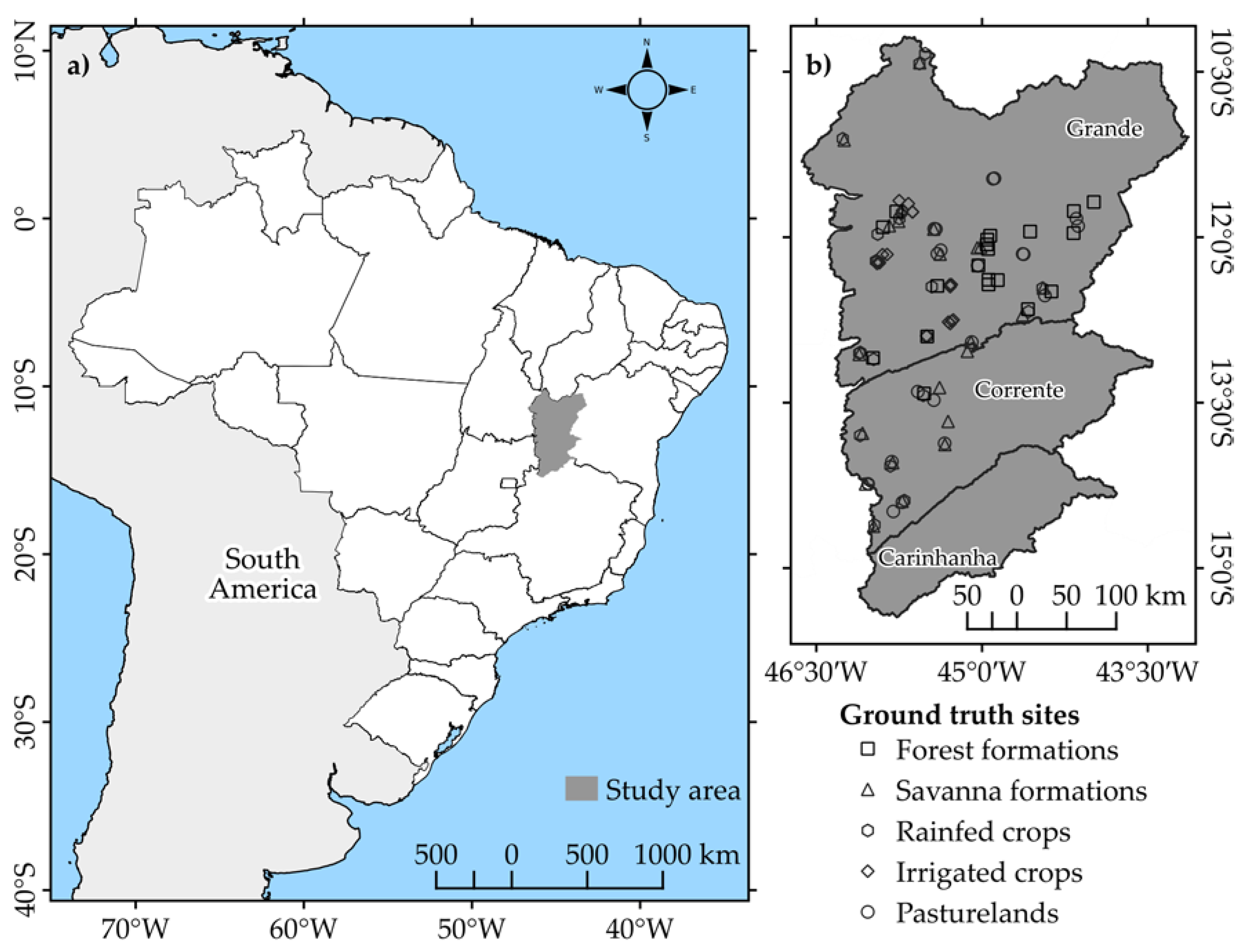
Western Bahia is part of MATOPIBA (acronym created from the first two letters of four Brazilian state names: Maranhão, Tocantins, Piauí, and Bahia), a region regarded as the last agricultural frontier in Brazil (Figure 1a). The region’s climate is not appropriate for producing two rainfed crops, but the rainy season is well defined. In addition, slopes vary from flat to wavy, facilitating large-scale agricultural mechanization. Finally, water resources are abundant, particularly in the extreme western part of the region [10], allowing for escalating irrigation growth since the 1990s [11]. These characteristics have attracted migrant rural producers from southern Brazil who established strong commercial agriculture in the region, although subsistence farming is also present. With only 1.5% of the national area, Western Bahia is today one of the largest producers of soybeans and cotton in the country.
2.2. Land Use and Land Cover Classification
Land use and land cover were classified into nine categories. The Cerrado biome’s natural vegetation is a mosaic of different vegetation types ranging from grasslands to forestlands. It has been classified into three categories by [12]: forest formations (ciliary forest, gallery forest, dry forest, and Cerradão), savanna formations (Cerrado sensu stricto, park savanna, palm, and vereda), and grasslands (campo limpo, campo sujo, and campo rupestre). Agriculture land uses include four classes [9]: rainfed agriculture, irrigated agriculture, pasturelands, and mosaics of crops and pastures. Water bodies and urban areas/other farm buildings complete the list.
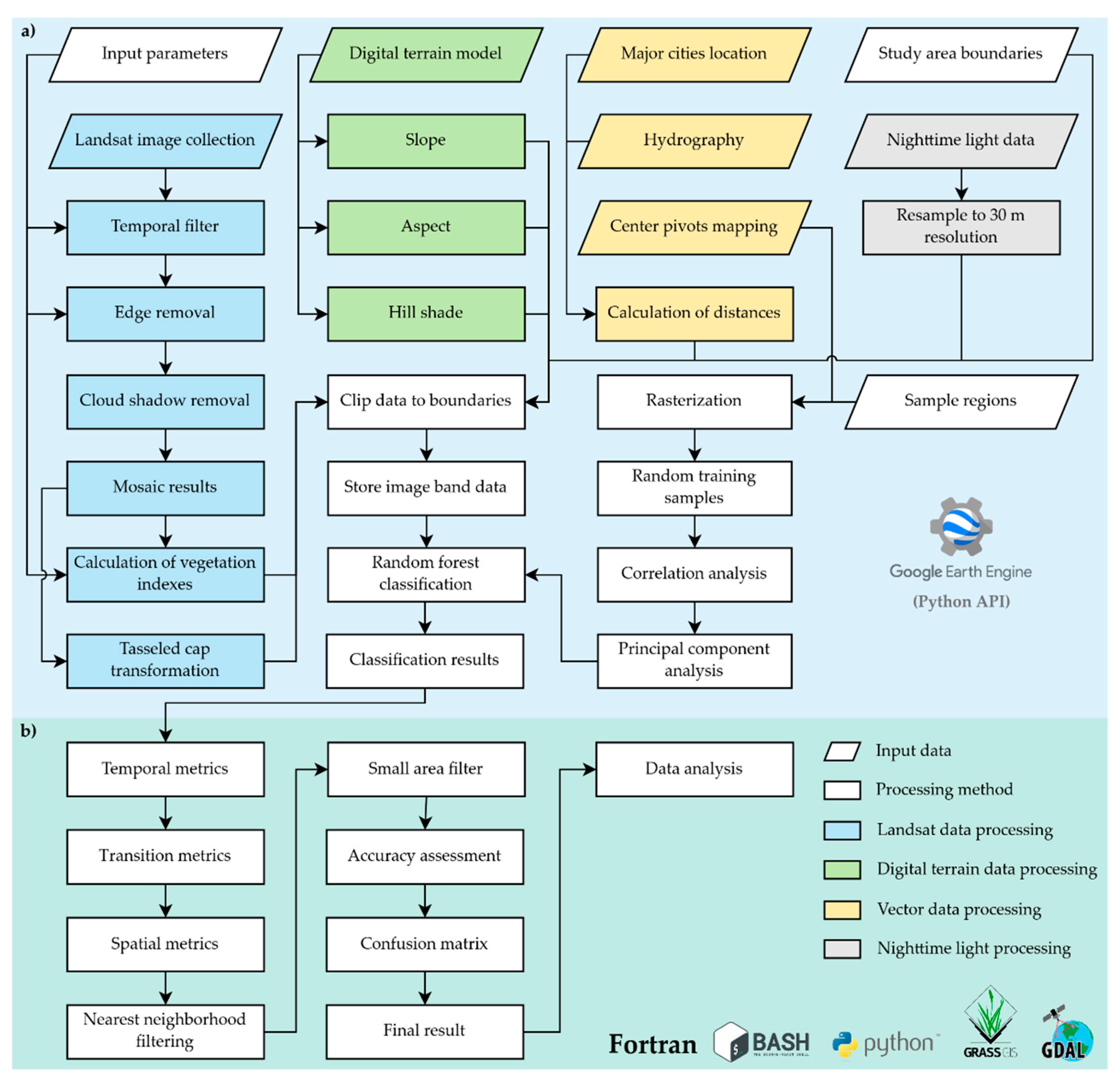
The land use and land cover classification (LULCC) method used includes cloud computing steps using the Python API on the Google Earth Engine platform [13] (Figure 2a) and local processing steps using a set of programming languages and open-source tools for geospatial analysis (Figure 2b).
The imagery dataset used in this work was composed by Thematic Mapper, Enhanced Thematic Mapper Plus and Operational Land Imager Landsat sensors, onboard Landsat 5, 7 and 8 missions [14]; the digital surface model used was ALOS World 3D-30m dataset, version 3.1 [15]; the Day/Night band composites of nighttime data from the Visible Infrared Imaging Radiometer Suit project (VIIRS), version 1.0 [16]. The urban and road infrastructure data were obtained from the OpenStreetMaps project database [17] and the hydrography data used was obtained from the multiscale ottocodified hydrographic base provided by the National Water Agency in Brazil [18]. Agricultural areas used to validate our study were provided from the Municipal Agricultural Survey—IBGE [19], MapBiomas version 4.1 [9], TerraClass project [20], and PRODES Cerrado [21].
The random forest classifier [22] was applied to Landsat 5, 7, and 8 images to produce the LULCC maps. Seven Landsat bands were used in this work, including visible (red, green, blue), near-infrared (NIR), shortwave infrared (SWIR1, SWIR2), thermal, in addition to pixel quality assessment. All images were filtered for the dry season of the Cerrado biome (from April to August) to minimize the commission errors in the classification of forest formations and to avoid loss of information due to clouds and cloud shadows. A total of 49,639 tiles were processed: 20 scenes to cover the entire study area annually from 1990 to 2020, with one image every 16 days for the seven Landsat bands used. Each image was corrected for top-of-atmosphere and relief (pixel-by-pixel approach), removing pixels contaminated by clouds and cloud shadows and, subsequently, the noise of images edges. Thirty-one annual mosaics were generated—from 1990 to 2020—using the median values of the pixels uncontaminated by clouds and cloud shadows filtered from the images time series.
In addition, forty indexes were calculated based on (i) Landsat 5, 7 and 8 bands, (ii) the ALOS World 3D-30m, (iii) the VIIRS Day/Night Band, and (iv) from the pixel distances to the main towns, rivers, and roads in the study area to be later evaluated against the random stratified samples generated within the polygons digitized in this work.
Three types of data sampling were used for calibration of the classification. First, we classified the land use and land cover for 120 ground truth sites in two field campaigns in 2017 [23] (Figure 1b). The land use and land cover were organized into five classes: (i) forest formations, (ii) savannas, (iii) rainfed crops, (iv) irrigated crops, and (v) pastures. These field samples were then used to assist in manually drawing 2707 similar polygons in neighbor regions of the mosaic generated for that year (112 polygons in forest formations, 121 in savanna formations, 121 in grasslands, 35 in mosaics of crop or pastures, 294 in rainfed crops, 1411 in irrigated crops, 309 in pasturelands, 204 in water bodies, and 100 in urban areas/farm buildings). Random pixels were sampled inside the drawn polygons (stratified sample approach) to expand the sampling points from 120 to about 28,500 points. These training data were sufficient to train the classifier, since the use of all pixels within the polygons made the computational processing time much longer.
Second, grasslands were sampled with Landsat images with a natural color composition and the normalized difference vegetation index. Third, urban areas and water bodies were sampled based on mapping data from the OpenStreetMap project and the Landsat NIR band. Regions that were not distinguishable between cropland and pasture were classified as a mosaic of crops and pastures.
Dimension reduction procedures such as a principal component analysis and a correlation analysis were performed to eliminate the calculated indexes with high autocorrelation (r > 0.75) for all sampling points. In addition, spectral information from Landsat data bands (blue, green, red, NIR, SWIR1, SWIR2) was transformed by the tasseled cap method into three indexes (brightness, greenness, and wetness), providing more specific spectral information [24,25,26,27]. After all processing, a combination of 14 bands and indexes was sufficient to classify the images: nighttime light data, normalized difference built-up index, four physical data variables (elevation, slope, aspect, and hill shade), pixel distances to the nearest stream, red/green ratio, enhanced vegetation index, normalized difference water index, the three tasseled cap transformation indexes, and a water mask.
To train the random forest classifier, we randomly selected 80% of all sampled points collected (22,800 points) and used 100 decision trees and the 14 indexes remaining after the dimension reduction procedures. Three thousand two hundred points were randomly stratified to train (800 for validation) each class of natural vegetation and agriculture, while just 200 points were randomized to train (50 for validation) water bodies and urban areas/agricultural buildings to minimize commission errors on these two classes.
Initially, the classifier was not able to identify irrigation areas with high accuracy. Most of the irrigation areas were originally classified as rainfed crops due to the similarity of the irrigated and rainfed area’s spectral response when there was no crop planted in the center pivots at the time the images were collected. Therefore, we separated the rainfed croplands from the irrigated farmlands using the maps of historical center pivot data in Western Bahia from 1990 to 2018 [11], which were also produced using remote sensing, ground-truth data, and cloud computing. Subsequently, the series with irrigated areas was digitized and updated with the years 2019 and 2020 in this work using the same methods according to [11].
The diverse spectral responses related to climate seasonality and interannual variability, variations within the same land cover class, different crops, and crop-pasture mosaics caused discontinuities in the classification results. To minimize these discontinuities, algorithms based on temporal, transition, and spatial metrics were developed. The temporal discontinuities associated with the interannual variability of climate and other variations in time were filtered using a 5-year filter (the year to be corrected, the two years before, and the two years after). The replaced pixel is equal to the statistical mode (the most common value) of the pixels within these five years. With this metric, it was possible to minimize the discrepancies of temporal continuity of LULCC classes due to failures in the acquisition of data from sensors and the presence of clouds and shadows. This process also reduces transition inconsistencies between the classes of forest and savanna formations attributable to variations in the greenness of the natural vegetation caused by the interannual variability of climate (e.g., it avoids unlikely changes such as forest formation > rainfed crop > forest formation). In addition, specific rules were used to correct the years at the beginning and end of the series (1990, 1991, 2019, and 2020). For example, for the year 1991, the metric correction used only the year 1990 and the two subsequent years. For 2020, the filter used only the previous two years of data.
Finally, spatial metrics were used to remove isolated pixels and small clusters of pixels (<1 ha, or <10 pixels) to generate the final time series dataset of LULCC from 1990 to 2020.
Two methods evaluated the accuracy of the land use classification: (i) a cross-comparison between ground-truth sites and the classification results using the Cohen’s kappa index [28,29], and (ii) correlations of total area per class against other LULCCs. These correlations were calculated at the municipality level, aggregating cropland and pastureland data results of this work and correlating them with four independent products for different periods. The first database used to evaluate LULCC was the IBGE (Brazilian Institute of Geography and Statistics) database for the period 1990–2018 [19]. The second was the LULCC time series from the MapBiomas consortium (release 4.1) for 1990–2018 [9]. The third was the municipality-aggregated yearly deforestation data from the PRODES Cerrado project during 2008–2018 [21]. The fourth was the agricultural land use data from the TerraClass project for the Cerrado for 2013 [20].
2.3. Suitability for Future Agricultural Expansion
The suitability analysis for future agricultural expansion was divided into five parts (Appendix A, Figure A1). First, the land suitability classes were defined following the Food and Agriculture Organization of the United Nations (FAO) land suitability classification: highly suitable, moderately suitable, marginally suitable, and unsuitable (Section 2.3.1). Second, the criteria used to identify suitability were chosen according to their importance for agricultural expansion in Western Bahia (Section 2.3.2). Third, the criteria and the pair-wise comparison matrix were aggregated and processed using the spatial multicriteria decision analysis (SMCDA) method applied to the 1990 LULCC. This step also eliminated the restricted areas from suitable areas for expansion (Section 2.3.3). Fourth, the areas classified according to their 1990 suitability were evaluated against historical land use changes (Section 2.3.4). Here, rainfed crops, irrigated crops, and pastureland areas were spatially associated with land suitability classes to assess agricultural expansion changes from 1990 to 2020. Finally, the criteria weights from the SMCDA method were also applied to 2020 LULCC to generate an updated suitability map for future agricultural expansion (Section 2.3.5).
2.3.1. Suitable Areas
The land suitability classification by the FAO approach classifies land according to a range—from highly suitable to not suitable (unsuitable)—based on climate, terrain, soil properties, and other land-use-related characteristics [30].
The quality of land suitability assessments, and hence the reliability of land use decisions, depends primarily on the quality of the information used to derive them [31]. Land evaluation is defined as “the assessment of land performance when used for a specified purpose, involving the execution and interpretation of surveys and studies of landforms, soils, vegetation, climate and other aspects of land to identify and make a comparison of promising kinds of land use in terms applicable to the objectives of the evaluation” [30]. Here, the lands are classified in only one kind of suitability class, described in Table 1.
2.3.2. Criteria Thresholds
To evaluate the land suitability for future agriculture expansion in Western Bahia, we used a SMCDA. SMCDA is a useful tool to assess multiple conflicting criteria in the decision-making process. It is mainly used when it is necessary to decide which metrics are most relevant or limiting in decision analysis. A detailed description of the SMCDA method and results are presented in Appendix A.
First, we used three criteria to determine the agricultural land suitability for cropland and pastureland in Western Bahia: (i) the percentage of years that the rainy season lasted longer than 120 days (pp), (ii) the 1990 LULCC, and (iii) the slope of the terrain. Then, we evaluated their influence on agriculture expansion in the region (Table 2).
We selected pp because the rainfed croplands are critically dependent on rains for healthy growth and production. Rainfed crops typically grown in the region, such as soy, cotton, or maize, require at least 600 mm of rainfall, which must be distributed throughout the 120-day growing season. The climate in Western Bahia presents substantial interannual variability, both in terms of the amount of annual rainfall and duration of the rainy season [8]. As a result, areas where the rainy season lasts at least 120 days every year (pp = 100%) are the best choice for a safe financial return and receive the highest suitability-priority value (1). In contrast, areas that meet this criterion less frequently receive lower suitability-priority values, according to Table 2. We also assumed that when the rainy season lasts longer than 120 days, the amount of rain exceeds 600 mm in the period. Fuzzified values associated with pp are presented in Figure A3a.
LULCC is a simple criterion to indicate how human activity interacts with the landscape. It is related to the cost of converting the natural land cover to agriculture and is also associated with land economic value. Agricultural lands undoubtedly have higher suitability values than the unconverted areas (forests, savannas, and grasslands), which have their suitability values chosen according to the cost of conversion, according to Table 2. A map of the fuzzy set for LULCC is similar to the land use map presented in Figure 3.
Finally, agricultural machinery increases farm worker productivity, and thus mechanization is another particularly important driver of productivity, land value, and suitability for agriculture. The slope has a sizable financial influence on agriculture production—large tractors and implements can only be used when the grade is low (<3%). In comparison, smaller and less productive tractors must be used as inclination increases until the maximum of 30% inclination, the practical limit for tractor use (Table 2). Fuzzified values associated with slope are presented in Appendix A, Figure A3b.
The agricultural suitability map for 2020, used for future expansion analysis, was generated with the same weights from the SMCDA based on the pp, slope, and LULCC criteria from 1990, changing only the LULCC map to 2020.
2.3.3. Constrained and Restricted Areas
Constrained areas are not subject to short-term changes; i.e., currently, they cannot be used for agriculture. They include urban areas, highways, farm buildings, and water bodies (small lakes, dams, or streams). Constructed areas, roads, and the stream network locations were produced as part of the land cover classification described in Section 2.2.
The restricted areas are lands intended for environmental preservation due to federal regulations and cannot be used for agriculture. These include Permanent Preservation Areas (PPAs), Legal Reserves (LRs), and Integral Conservation Units (ICUs). PPA and LR are regulated by Brazil’s revised Forest Code (Federal Law 12,651 of 25 May 2012), whereas ICUs are governed by the National System of Nature Conservation Units (Federal Law 9985, of 18 July 2000).
PPAs are natural landscapes preserved mainly due to the natural vegetation’s capacity to protect the soil against erosion, landslides, or other forms of degradation. It covers geologically fragile spaces such as river edges and mountain tops, among others and helps preserve water resources and biodiversity, facilitating fauna and flora’s gene flow.
LRs are areas with native vegetation located inside a rural private property, other than the PPAs. They are necessary for the sustainable use of natural resources, helping in the conservation and rehabilitation of ecological processes and promoting the preservation of biodiversity and shelter and protection of wild fauna and native flora. In the Cerrado biome, rural properties must preserve at least 20% of the total property area as a LR. Although the legislation allows the possibility of sustainable management of the LR under specific conditions, we decided to keep these areas entirely restricted from agricultural expansion in our land suitability classification.
ICUs are set aside to preserve nature, and only the indirect use of their natural resources is allowed, with exceptions specified in the legislation. Agricultural activities are not permitted in an ICU. Thus, we consider these areas as restricted from agriculture expansion.
PPAs, LRs, ICUs, constructed areas, highways, and stream network locations were converted to raster format in the same resolution as the LULCC and were aggregated to the SMCDA.
2.3.4. Evaluation of Results
To evaluate the suitability analysis’s accuracy for future agricultural expansion classification, we compare the actual land use classification for 2020 against the land suitability classes for 1990. This analysis assesses how the LULCC observed in 2020 is distributed across the land suitability classes determined 30 years before.
2.3.5. Assessment of Future Expansion
The validated criteria weights from the SMCDA method were also applied to the 2020 LULCC to generate the 2020 suitability map. The 2020 map is different from the 1990 map because changes in land use and land cover may have changed the land suitability, following the rationale of Table 2.
The agricultural suitability changes in the last 30 years are analyzed by a cross-comparison of the suitability maps of 1990 and 2020 (Section 3.2).
To assess the limitations on future agricultural expansion, we cross-evaluate agricultural lands with irrigated crops considering both the agricultural suitability level of the remaining areas (i.e., those that have not yet been converted to agriculture) and the restrictions related to conservation units and preservation areas.
3. Results
3.1. Land Use and Land Cover Classification
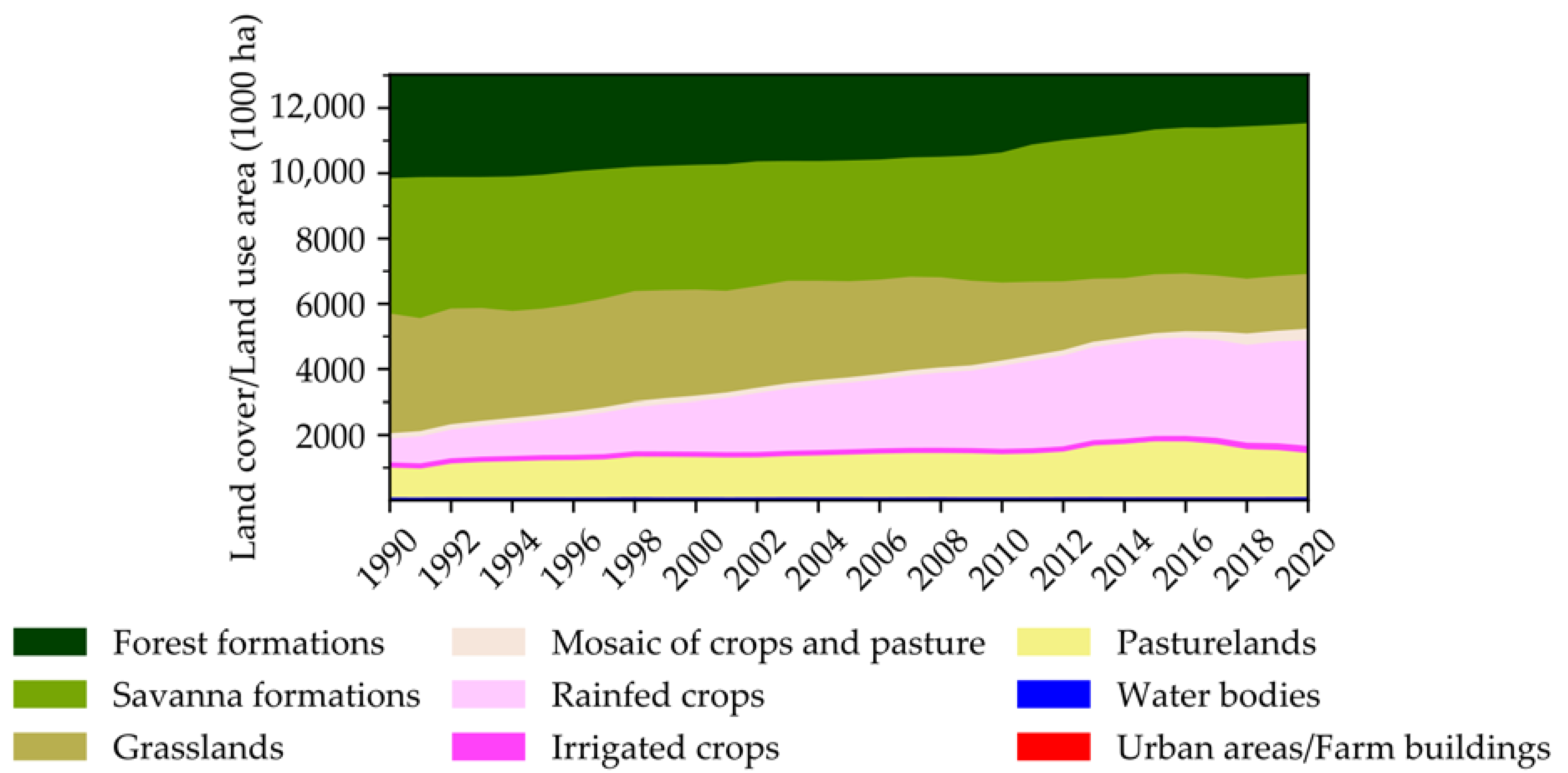
The historical LULCC dataset has a yearly temporal resolution (from 1990 to 2020) and a spatial resolution of 1 arc-second (approximately 30 m). The historical series contains the following classes: forest formations, savanna formations, grasslands, mosaics of crops and pasture, rainfed crops, irrigated crops, pasturelands, water bodies, and urban areas/farm buildings. Agricultural expansion occurred mainly from west to east in the region (Figure 3a–g). In the extreme western areas, most landscapes classified as pastureland in 1990 were converted to rainfed croplands by 2005 (Figure 3a–d). The expansion of rainfed agriculture in the extreme west has dislocated pasturelands mostly to the northeast and southeast. Most savanna formations were converted to pastures, while the grasslands were converted to croplands (Table 3). The growth of irrigated cropland in the region occurred mainly between longitudes 46°W and 45°W on the plateau (Figure 3a–g). The irrigated cropland spread between 12°S and 13°S in the late 1990s (Figure 3b,c), later intensified in these areas (Figure 3d,e), and more recently expanded to other regions (Figure 3f,g).
The transitions between the land use and land cover classes are shown in Table 3. Overall, the total agricultural area expanded from 1.97 Mha in 1990 to 5.14 Mha in 2020, an increase of 3.17 Mha (average expansion rate of 102,269 ha yr−1, or 3.14% yr−1 from 1990 to 2020) (Table 3 and Figure 4). Irrigated croplands increased 7.35% yr−1, from 2.42 × 10⁴ ha to 2.18 × 10⁵ ha (from 187 center pivots in 1990 to 1883 center pivots in 2020) (Table 3).
At the decadal time scale, the total agriculture areas increased by 1.13 Mha in 1990–2000, 1.07 Mha in 2000–2010, and 0.970 Mha in 2010–2020. The average linear expansion rate has decreased slightly in the period (0.112, 0.107, and 0.097 Mha yr−1, respectively), but the decadal growth rate was approximately twice as high in 1990–2000 (57%) as the growth rate in 2000–2010 (35%) and 2010–2020 (23%). Rainfed crops increased by 0.833, 0.958, and 0.606 Mha from 1990–2000, 2000–2010, and 2010–2020, respectively, with a higher linear expansion rate in the first two decades (0.0833, 0.0958, and 0.0606 Mha yr−1, respectively) and a decadal growth rate of 102%, 58%, and 23%, respectively. Irrigated crops started from 24,200 ha in 1990 and increased by 49,700 and 34,600 ha from 1990-2000 and 2000-2010, respectively but accelerated to a change of 109,000 ha during 2010-2020, with growth rates of 205%, 47%, and 101%, respectively. Pasturelands had the highest growth in 1990-2000, increasing 0.274 Mha (27,400 ha yr−1, or 26% in 10 years), over five times higher than in 2000-2010 (4,980 ha yr−1, or 4% in 10 years). After that, pasturelands decreased at the rate of 2110 ha yr−1 during 2010-2020.
The next paragraphs analyze the long-term changes, i.e., from 1990 to 2020, according to the conversion matrix presented in Table 3.
The rainfed crop areas increased by 2.39 Mha, from 0.817 Mha to 3.21 Mha (7.72 × 10⁴ ha yr−1). This increase represents 76% of the overall agricultural land expansion (3.17 Mha; Table 3 and Figure 4). Over time, rainfed crops were established mostly over grasslands (9.00 × 10⁵ ha) and savanna formations areas (6.88 × 10⁵ ha), with smaller areas coming from forest formations (4.98 × 10⁵ ha) and pasturelands (3.33 × 10⁵ ha) (Table 3).
Total pasturelands area increased by 300,000 ha, from 1.05 Mha in 1990 to 1.35 Mha in 2020 (an average rate of 9.75 × 10³ ha yr−1, which represents 10% of the overall agriculture expansion) (Table 3). The pasturelands expansion occurred mainly in savanna areas (5.64 × 10⁵ ha), with smaller areas coming from forest formations (1.07 × 10⁵ ha) and grasslands (1.01 × 10⁵ ha).
Mosaics of crops and pasture increased by 277,700 ha, from 7.63 × 10⁴ ha to 3.54 × 10⁵ ha in 2020 (8.97 × 10³ ha yr−1), mostly over savanna formations (1.31 × 10⁵ ha) and forest formations areas (5.30 × 10⁴ ha). Most irrigated crops were established on grassland and savanna formations (7.34 × 10⁴ ha and 6.29 × 10⁴ ha, respectively).
Meanwhile, natural vegetation decreased by 3.18 Mha, from 11.0 Mha in 1990 to 7.87 Mha in 2020. Forest formations decreased by 1.69 Mha and grasslands decreased by 1.96 Mha, while savanna formations increased by 470,000 ha. The slight increase in the savanna formations area seems to be due to the degradation of forest formations caused by fire or other disturbance: 1.15 Mha of forest formations were converted to either savanna (1.11 Mha) or grasslands (41,600 ha). A much smaller portion of forest formations was converted to pastureland (107,000 ha), rainfed crops (498,000 ha), and irrigated crops (20,600 ha). Urban areas and farm buildings increased from 3510 ha in 1990 to 11,400 ha in 2020 (Table 3).
These numbers indicate a change in the agricultural focus of the region. While pasturelands dominated in 1990 (1.05 Mha versus 0.82 Mha), rainfed crops were predominant in 2020, with twice as much cropland as pasture (3.21 Mha versus 1.35 Mha). About 343,000 ha of cropland area (333,000 ha of rainfed and 9,700 ha of irrigated) were established over former pasturelands. This accounts for about 33% of the total rainfed agriculture expansion of 1.05 Mha. Moreover, the high rate of irrigation growth—nearly twice as fast as rainfed cropland expansion (7.35% yr−1 versus 3.14% yr−1)—also illustrates the region’s investment in irrigation.
In summary, the agricultural expansion occurred mainly over grasslands and savanna formations, while part of the savanna loss was offset by the degradation of forest formations to savanna formations (Table 3 and Figure 4). In addition, agricultural expansion slowed between 2013 and 2015, and since 2015, it appears to have stabilized.
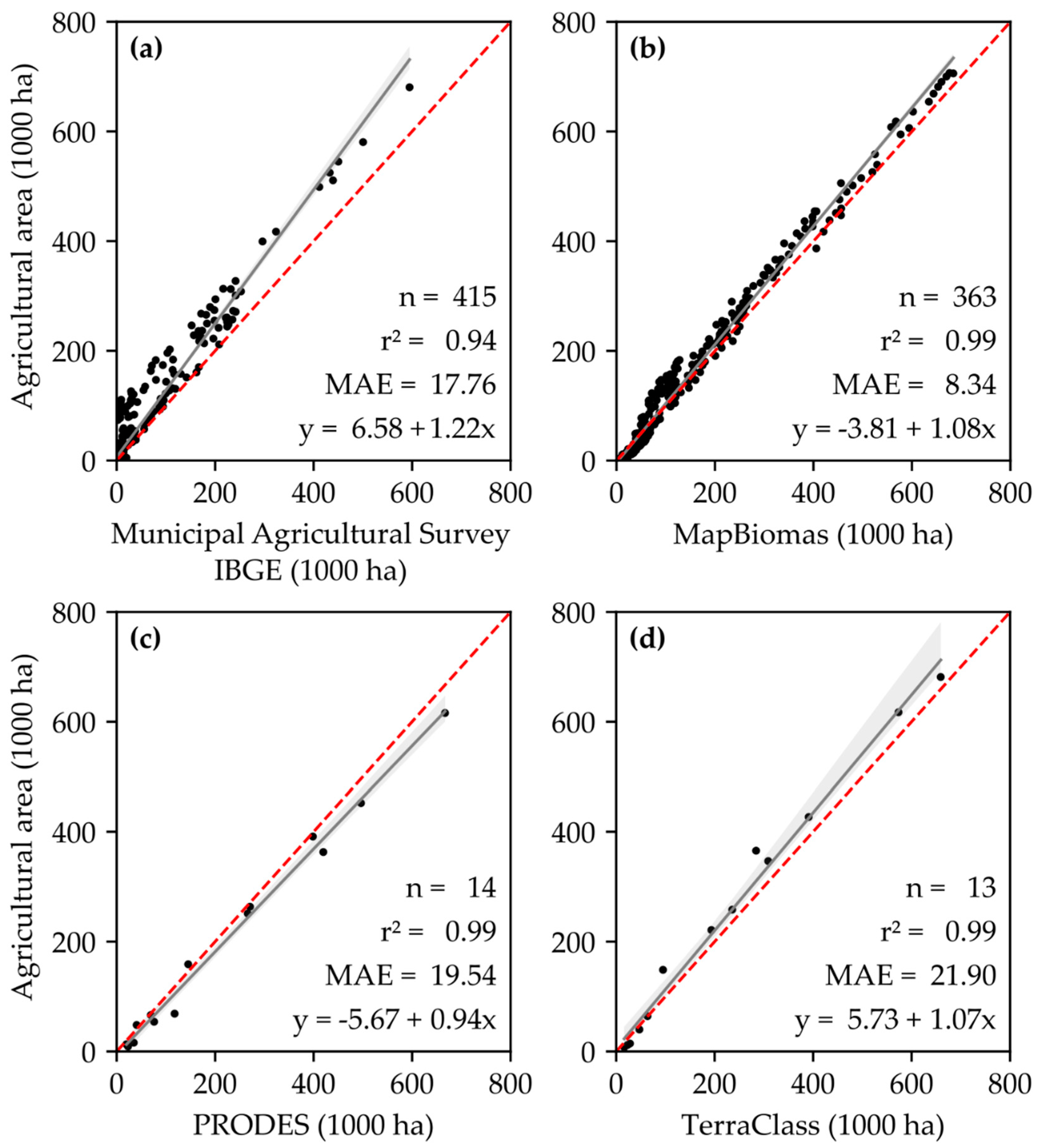
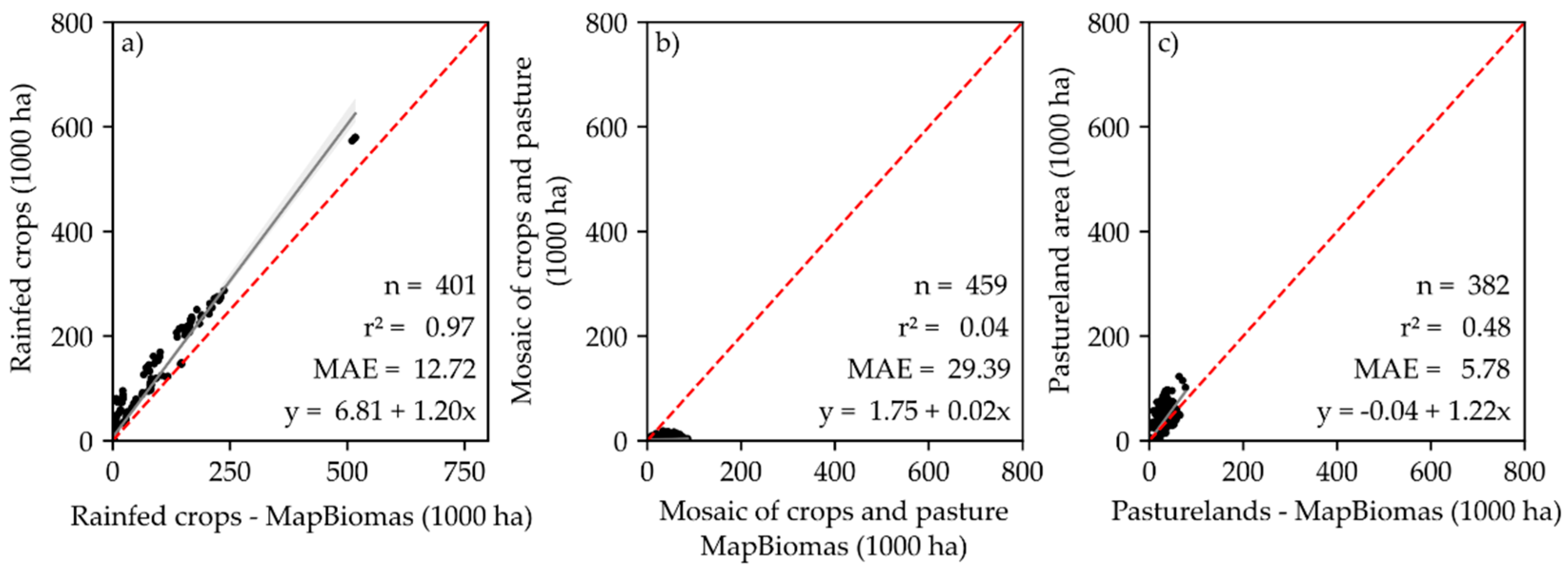
The accuracy of the LULCC was determined by -cross-comparison of the municipality-aggregated LULCC data from different databases. The Cohen’s kappa, although it was a classic accuracy index widely used in remote sensing in the past, was not used in this work because it is misleading and/or incorrect for practical applications in remote sensing [32,33]. A more robust indicator of accuracy is the determination coefficient r2, which was used to determine all correlations between agricultural areas from our LULCC database (y-axis) and other LULCC data (x-axis). In all cases, r2 was higher than 0.94 (Figure 5a–d).
Compared to the MapBiomas 4.1 classification, the LULCC developed in this study showed an adjustment of r2 = 0.97 for the rainfed crop class (Figure 6a), r2 = 0.04 for mosaics of crops and pastures (Figure 6b), and r2 = 0.48 for the pastureland class (Figure 6c). The rainfed crops and pastureland areas were slightly overestimated in our LULCC (slope ~1.2) (Figure 6a,c). The differences between our results and MapBiomas are also influenced by ground truth data used for machine learning calibration of the classification algorithms. While our analysis is regionally focused, using ground truthing throughout the region to improve the classifier, MapBiomas analysis is nationally focused and may underperform in a specific region.
3.2. Suitability for Future Expansion
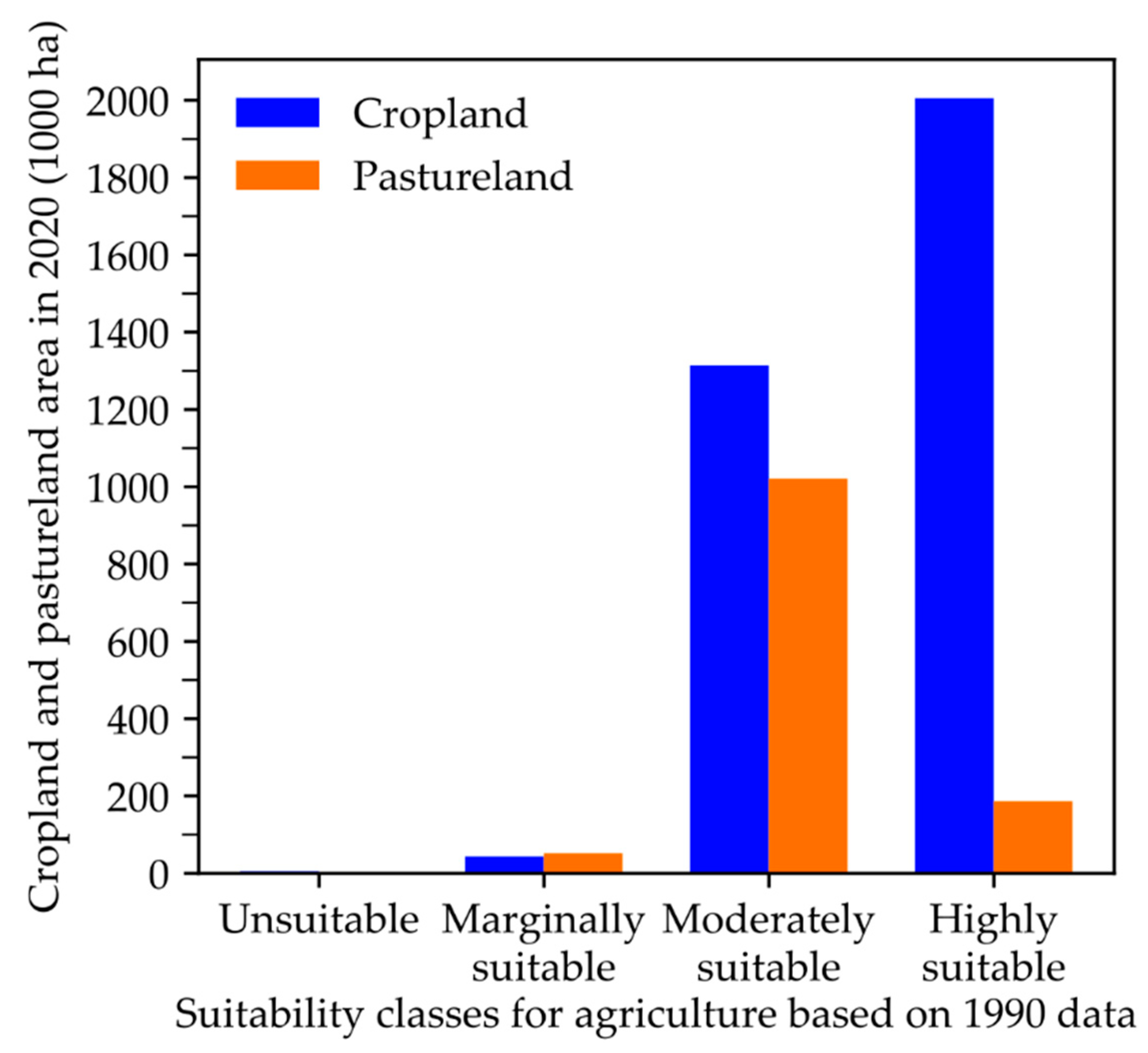
A map of agricultural suitability in 1990 is presented in Appendix A, Figure A2a. The areas classified according to their 1990 suitability are evaluated against historical land use changes (Figure 7). In 2020 the highly suitable lands were mainly used by croplands (both rainfed and irrigated), with a small number of pasturelands in these lands. On the other hand, moderately suitable areas are somewhat well distributed between pasturelands and croplands. The fact that most of the highly suitable land was taken over by croplands validates our land suitability analysis.
In 2020, 2.00 Mha of cropland areas occupied highly suitable areas, while 1.31 Mha occupied moderately suitable areas (Figure 7). The pasturelands are located mainly in moderately suitable areas (1.02 Mha), and a lower amount is in highly suitable areas (0.186 Mha). The presence of agricultural practices in marginally suitable and unsuitable areas in Western Bahia represents less than 105,000 ha (Figure 7). While marginally suitable cropland areas represent 43,700 ha and pasturelands a total of 52,000 ha, the use of unsuitable areas by crops and pastures is negligible.
The transitions of cropland, pastureland, and remaining natural vegetation areas (i.e., those that may have remaining potential for conversion to agriculture) followed different pathways between the suitability classes. We showed in Section 3.1 that total cropland in Western Bahia increased from 0.841 to 3.43 Mha (Table 3). Most of this expansion (2.39 Mha) happened in highly suitable areas (from 0.77 Mha in 1990 to 3.17 Mha in 2020; Table 4). In the moderately suitable areas, cropland increased from 25,900 ha to 197,000 ha, while in the marginally suitable areas, it increased from 794 ha to 7960 ha (Table 4).
Pastureland increased by 300,000 ha from 1990 to 2020. It has expanded mainly in moderately suitable areas, increasing from 480,000 ha in 1990 to 824,000 ha in 2020 and in the marginal areas from 2780 ha to 4480 ha. However, in highly suitable areas, pasturelands decreased from 483,000 ha to 438,000 ha (Table 4).
Natural vegetation was mostly present in highly and moderately suitable areas in 1990, and thus these were the lands that suffered most of the conversion to agriculture (changes of −1.39 Mha and −1.08 Mha, respectively; Table 4). In 1990, the remaining natural vegetation areas were predominantly in moderately suitable areas rather than in highly and marginally suitable areas; this general pattern persisted in 2020. In 1990, 6.10 Mha of the remaining natural vegetation area was in the moderately suitable class, followed by 2.05 Mha in highly suitable areas and 644,000 ha in marginal areas. In 2020, the natural vegetation areas decreased to 5.02 Mha in the moderately suitable class, 659,000 ha in the highly suitable class, and 256,000 ha in marginal areas.
Overall, the total agricultural area increased by 2.88 Mha at the expense of natural vegetation. Of these changes, 83% (2.39 Mha) were for establishing croplands in highly suitable areas (Table 4). Little highly suitable land remains unused by agriculture today (657,000 ha). As discussed in the previous paragraph, most of the land available for expansion is moderately suitable for agriculture (5 Mha, Table 4). However, 94% of 2020 croplands (3.17 out of 3.43 Mha) are in highly suitable areas, which reflects the preferences of crop farmers for better lands and sets limitations for cropland expansion in the region. These limitations will be discussed in Section 4.
An analysis of the spatial patterns of agricultural land use across suitability classes indicates that croplands and pasturelands dominated most of the highly suitable areas in 1990 (compare dark green shades in Figure 8a with dark blue shades in Figure 8b). Some highly suitable areas initially used as pasturelands were converted to croplands throughout the years, for example, in the extreme west around 13°S. In 1990, most of the remaining unused areas were classified as moderately and marginally suitable areas that were subsequently converted to crop or pasture over time (Figure 8, Table 4). Pasturelands expanded over moderately suitable areas (Figure 8, Table 4) and diminished over highly suitable areas, indicating that farmers replaced pastures located in highly suitable areas with croplands (Figure 8).
The rainfed cropland in highly suitable areas increased at an approximately constant rate (4.40 × 10⁴ ha yr−1) from 1990 to 2013. From 2013 to 2018, this rate decreased to 2.81 × 10³ ha yr−1 (Figure 9a), and after 2018, it increased to 8.70 × 10³ ha yr−1. This dramatic decrease between 2013 and 2018 is most likely associated with the new Forest Code’s approval and the scarcity of highly suitable land discussed above. However, it is also linked with agricultural intensification practices such as irrigation, which has also increased dramatically since 2013 (Figure 9b). In other words, without much highly suitable land available for expansion and pressured by the Forest Code limitations, farmers increasingly turned to irrigation to increase production.
Similar patterns were observed on rainfed crops in moderately suitable regions (Figure 9a). From negligible amounts in 1990, rainfed crops expanded into moderately suitable areas at a rate of 4.01 × 10⁴ ha yr−1 until 2013, reaching 0.962 Mha. From 2013 to 2018, this rate decreased to 1.38 × 10⁴ ha yr−1, and then it increased again after this period (Figure 9a). Moreover, since rainfall limitation is one the major limitations on land suitability in this region, irrigated crop area increased nearly as fast in moderately suitable lands as in highly suitable lands.
Irrigated crops increased by 2110 ha yr−1 in highly suitable areas and 1700 ha yr−1 in moderately suitable areas from 1990 to 2011, increasing irrigated area by 46,500 ha in highly suitable areas and by 37,500 ha in moderately suitable areas. Between 2011 and 2020, irrigated crops expanded twice as fast, increasing by 61,400 ha (6140 ha yr−1) in highly suitable areas and 42,900 ha (4290 ha yr−1) in moderately suitable areas. There is little irrigation on marginally suitable lands (Figure 9b). This confirms irrigation as a solution to increase production in a scenario with low availability of highly suitable land and to overcome rainfall limitations in moderately suitable lands.
Pasture area, on the other hand, decreased from 1990 to 2012 in highly suitable areas at a rate of −11,600 ha yr−1 (from 481,000 ha to 215,000 ha), while increasing in moderately suitable areas at a rate of 25,800 ha yr−1 (from 478,000 ha to 1.07 Mha). From 2012 to 2015, the pastureland growth rate in moderately suitable areas increased further to 55,300 ha yr−1, while shifting to positive growth rates in highly suitable areas (+5990 ha yr−1). After 2015 the pasture area started to decrease dramatically, with a negative growth rate of −8720 ha yr−1 in highly suitable areas and −45,100 ha yr−1 in moderately suitable areas. Marginally suitable areas had little importance for pastures.
The region’s commitment to grain and fiber production was demonstrated by the steady growth in rainfed and irrigated crop areas after 1990 and the steady decrease in pasturelands in highly suitable areas. However, after the mid-2000s, pastures increased quickly in the moderately suitable areas in the northeastern part of the region (Figure 9c but see Figure 3 and Figure 8). As stated earlier, from 1990 to 2012, pasturelands grew consistently on moderately suitable areas (25,800 ha yr−1) with a substantial increase in the rate between 2012 and 2015 (55,300 ha yr−1), followed by a decrease again after 2015. Despite the twofold increase in a short period (2012 to 2015), pasturelands have been replaced by rainfed and irrigated crops. Pasturelands represent a small fraction of croplands and typically occupy areas with precipitation restrictions, which are unlikely to be used by rainfed croplands.
4. Discussion
The evolution of land use in Western Bahia is following two notable patterns. First, cropland has established itself primarily in the flat, rainy, and highly suitable areas of the extreme western part of the region. It confirms the results of previous studies that have analyzed agricultural expansion in specific municipalities, like São Desidério [35], Barreiras [36], Riachão das Neves [37], and Formosa do Rio Preto [38]. In earlier years, it expanded somewhat linearly, with subsequent expansion in moderately suitable areas. Pasturelands occupy other moderately and marginally suitable areas. This linear expansion lasted until about 2012–2013. The subsequent slowdown in the extensification trend was due to a combination of a scarcity of highly suitable area (only 0.657 Mha, Figure 10) and the approval of Brazil’s new Forest Code in 2012. The impact of the Forest Code is clearly visible in Figure 10. There is twice as much area preserved as remaining highly suitable areas for agriculture expansion. On the other hand, plenty of moderately suitable areas remain available (5.00 Mha, Figure 10), but farmers clearly prefer to expand production by increasing irrigated area (Figure 10).
As discussed above, nearly all the land available for expansion is moderately suitable for agriculture, which has been similarly used by rainfed croplands and pasturelands (Figure 7). The environmental impacts of a possible agriculture expansion in the region have been discussed somewhat generically due to the scarcity of regionally specific data for a thorough evaluation. For example, Gaspar et al. [39] argue that preserved areas may contribute to the maintenance of local biodiversity and the recharge of the Urucuia aquifer, while Oliveira et al. [40] conclude that the landscape transformation in Western Bahia has negative consequences on the ecosystem functioning. The most detailed data available is about the impacts of LULCC on changes in soil carbon storage. Conversion of Cerrado formations to irrigated croplands, rainfed croplands, and pasturelands does not significantly change the soil carbon content to a depth of 1 m (p-value = 0.33, 0.25, and 0.11, respectively) [41]. Moreover, 0-20 cm soil carbon volumetric content may significantly increase by 3% yr−1 in well-managed rainfed cropland clayish soils (p-value = 0.001) and by 2.6% yr−1 in irrigated areas (p-value = 0.057) [42]. The main problem is converting forested lands to rainfed croplands and pasturelands, which decrease soil carbon by 30% (p-value = 0.018) and 37% (p-value = 0.007), respectively [41]. Although most of the forest formations in the region are protected in LRs and PPAs, there are plenty of unprotected forest formations. Most of the original forest formations in 1990 have been degraded to savanna formations (probably through fire) or converted to pasturelands in 2020 (Figure 3, Table 3).
The second main pattern is the expansion of irrigated agriculture. The region’s location on the top of the Urucuia aquifer, the availability of vast surface water resources, and the flat topography have promoted this expansion. While the trend in the rainfed crop areas increased until 2012 and nearly leveled off after that (Figure 9a), the rate of expansion of irrigation after 2011 was about three times higher than the rate before 2010, occurring mainly in highly and moderately suitable areas (Figure 9b). The increase in investments in irrigation in this period may also have been encouraged by the 2013 National Policy on Irrigation (Law 12,787 of 11 January 2013), which provided several incentives for the expansion of irrigated area nationally, including subsidized rates on loans and reduced tariffs on electric power for irrigation projects. While Forest Code restrictions may have limited or at least discouraged extensification to new suitable lands, increasing cropping frequency through irrigation maintained the increasing trends in the region’s total agricultural output. To be sure, these changes in the last ten years have happened while there has been plenty of moderately suitable land for expansion (5.00 Mha, Figure 10).
Increasing production by irrigation—rather than by increasing cropped area—is also a smarter solution from both logistical and climate-risk points of view [43]. From a single farmer’s perspective, managing a single farm with irrigation and growing two high-yield crops on it in a year is much simpler than managing two rainfed farms of similar size that could be quite distant from one another. It avoids, for example, the purchase of duplicate machinery or the constant transport of machinery between farms. Moreover, rainfed crops are subject to crop failures in the event of prolonged dry spells or short rainy seasons—a somewhat common climatic feature in moderately suitable areas (as explained in Table 1 and Table 2).
On the other hand, the environmental consequences of choosing irrigation instead of extensification are different, and there are both positive and negative consequences. Choosing irrigation decreases the pressure on deforestation and carbon emissions associated with clearing land. Moreover, a recent study using eight years of soil carbon data in Western Bahia has shown that soils under irrigated croplands take up carbon at a rate of 0.28 g dm−3 yr−1 (2.6% yr−1, p = 0.065). In contrast, sandy soils under rainfed crops were not significantly accumulating carbon [42].
Irrigation, however, consumes water, which is a finite resource. Irrigation expansion is limited not only by slope but also by the availability of infrastructure and water resources. The potential for the development of irrigation in the area is currently unknown. Still, at least three sub-basins in Western Bahia are either in a state of conflict for water use or are moving rapidly toward it: The upstream Rio Grande, the Rio de Janeiro, and the Rio Branco (black polygons in Figure 8c). In these three sub-basins, the potential for expansion of irrigation is extremely low, if not null. These three sub-basins account for only 21% of the region’s area. Despite the high water stress, water use for irrigation has been steadily increasing, pushing the water stress to its limits [34], mainly in the basin’s headwaters. Most of the remaining moderately suitable areas for expansion are in the lower part of the Grande and Corrente basins, which do not include the three sub-basins discussed above (see overlap in Figure 8c). Although irrigation expansion along the main stems of the Grande and Corrente Rivers is a possibility, only a detailed water resources study will be able to quantify the maximum irrigated area in the region.
5. Conclusions
Expansion of the agricultural frontier and irrigation in both highly and moderately suitable areas has raised Western Bahia’s national and international importance. Most highly suitable land is already being used for agriculture—mainly as highly productive croplands, particularly soybeans and cotton. In response to the scarcity of highly suitable land, the limitations imposed by the new Forest Code around 2012, and energy tariff incentives to irrigation after 2013, farmers invested in cropland intensification through investments in irrigation systems, which increased output, simplified individual logistics, and stagnated deforestation.
Agricultural output in Western Bahia can increase by any combined pathway of area expansion or irrigation expansion (Figure 10, upper right side). Even considering the Forest Code and Conservation Unit restrictions, the agricultural area could nearly double in the region (Figure 10). However, the possible area expansion is mostly in moderately suitable areas, subject to climate hazards for rainfed crops but otherwise fine for pastures and irrigated crops, which are less susceptible to soil moisture limitations. Nevertheless, future land cover and land use changes may affect local biodiversity, aquifer recharge, ecosystem functioning, the local climate, and soil carbon storage. Thus, we emphasize the necessity of further regional studies to quantify the impacts of land use change in these interactions to contribute to the development of a more sustainable agricultural output.
Suppose future trends follow the trends of the last ten years (2011–2020). In that case, the main strategies to maintain the regional focus on crop production will be increased irrigation and conversion of the few pasturelands on highly suitable lands to croplands. At the same time, pasturelands may expand over the remaining moderately suitable areas.
Irrigation expansion, however, is contingent upon the availability of water resources and effective water security. Parts of the region, including most of the upstream Rio Grande basin and part of the Corrente basin, are already at water stress limits [11,34]. Although it has been strong in the last ten years, we urge that future irrigation expansion is preceded by careful planning and monitoring to avoid water insecurity in the region.
Author Contributions
Conceptualization, project administration, and funding acquisition, M.H.C.; field data collection: E.A.D. and M.H.C.; image processing, SMCDA and statistical analysis: F.M.P. and A.T.S.; writing—original draft preparation, F.M.P., A.T.S., M.H.C. and E.A.D.; writing—review and editing, F.M.P., A.T.S., M.H.C. and E.A.D. All authors have read and agreed to the published version of the manuscript.
Funding
This research was funded by PRODEAGRO, grant numbers 011/2016 and 045/2019, and by CNPq, process 441210/2017-1.
Data Availability Statement
Historical LULCC datasets and the agricultural suitability data developed in this work are available for visualization and download at the OBahia Platform (http://obahia.dea.ufv.br (accessed on 11 March 2021)).
Acknowledgments
Everardo C. Mantovani, Gerson C. Silva Jr., and Eduardo A. G. Marques have read and commented on previous versions of this manuscript. We thank them for their time and expertise.
Conflicts of Interest
The authors declare no conflict of interest. The funders had no role in the design of the study, in the collection, analyses, or interpretation of data; in the writing of the manuscript, or in the decision to publish the results.
Appendix A. Spatial Multicriteria Decision Analysis (SMCDA)
To develop a SMCDA, we used the analytical hierarchy process (AHP) with the ordered weighted average (OWA) in conjunction with programming languages and open-source tools for geospatial analysis.
The AHP is a decomposition multiple-attribute decision-making method that provides a comprehensive and mathematical structure to incorporate measures from objective criteria and derives priorities for intangible criteria to allow the best choice to be made in a decision process [44,45,46]. The AHP technique is useful due to its high accuracy for treating multiple criteria and compensating for both quantitative and qualitative data [47]. The calculated weights are not fuzzy numbers, which means that the results do not need to undergo defuzzification [48]. With the AHP method, it is possible to calculate the consistency ratio (CR). The criteria priorities are computed using a reciprocal pair-wise comparison matrix following the methodology proposed by [49].
The OWA is a parameterized family of combined operators that provides a general class of average aggregation operators. These operators allow the continuous adjustment of the values of the risk and tradeoff axes between the criteria, providing control over both the risk and tradeoff axes, which delimit the strategic decision space. The OWA method quantitatively considers degrees of optimism/pessimism and the effects of the decision maker’s different risk attitudes in a decision space. The OWA is characterized by two sets of weights: criterion importance weights and order weights.
The integration of the AHP with the OWA used in conjunction with programming languages and open-source tools for geospatial analysis presents an effective multicriteria decision analysis instrument for challenges oriented to make complex spatial decisions [50,51,52,53,54]. The SMCDA process used in this work is depicted in Figure A1.
Figure A1.
The spatial multicriteria decision analysis (SMCDA) model development flow. (a) Identification and contextualization of the problem. Definition of the criteria/metrics that significantly influence the model and definition of its priorities. (b) Assembling the pair-wise matrix with weights for each metric. Calculation of criteria maps (using fuzzy sets) to be used as inputs for analytical hierarchy process (AHP) and ordered weighted average (OWA) methods in geospatial analysis routines. This process generated a continuous map with values from 0 to 1, which is reclassified into suitability classes (4-highly suitable, 3-moderately suitable, 2-marginally suitable, and 1-unsuitable). At the end of the process, a mask was made to remove the preservation areas, conservation units, farm reserves, highways, hydrography, and urban areas. (c) Validation and statistical analysis of the suitability map results.

Appendix A.1. Weight Analysis
In AHP, the pair-wise comparison matrix is established based on opinions that, in most cases, have nonobjective nature. Therefore, any misjudgment parameters can be transferred to the score assignment and weights designation [55]. Three criteria were established to obtain a more consistent pair-wise matrix (pp, LULCC, and slope), which were identified according to stakeholder analysis (Figure A1a). Table A1 represents the pair-wise comparison judgment matrix (A = aij) evaluation of the criteria based on stakeholder analysis.

Table A1.
Pair-wise comparison matrix.
| Criteria | pp | LULCC | Slope |
|---|---|---|---|
| pp | 1 | 2 | 8 |
| LULCC | 1/2 | 1 | 5 |
| Slope | 1/8 | 1/5 | 1 |
| Sum | 1.625 | 3.200 | 14.0 |
Comparing all three criteria using the pair-wise comparison matrix provides the relative importance of each criterion toward others. For example, pp is eight times more important than slope and two times more important than LULCC.
The weight analysis to determine the degree of importance for each variable in the agricultural suitability classification confirm our hypothesis that pp is the most important criterion for agricultural suitability classification (60.4%), followed by the LULCC (32.6%) and slope (7%) (Table A2).
Table A2.
Normalized pair-wise comparison matrix.
| Criteria | pp | LULCC | slope | Weight |
|---|---|---|---|---|
| pp | 0.615 | 0.625 | 0.571 | 0.604 |
| LULCC | 0.308 | 0.313 | 0.357 | 0.326 |
| slope | 0.077 | 0.062 | 0.072 | 0.070 |
| Sum | 1 | 1 | 1 | 1 |
Appendix A.2. The Multiobjective Decision-Making Process
The AHP method used in this work was proposed by [56] and performs the following steps to ascertain the weights for each criterion (Figure A1b):
- Definition of the (n × n) pair-wise comparison matrix according to Table A1, where n is the number of criteria.
- Computation of the importance weight of each entry in column j of A by the sum of the entries in column j. This results in a normalized matrix (Awn×n).
- Computation of the ci values as the average of the entries in row i of Awn×n to yield the column vector Cn×1.
- Computation of the vector Xn×1 = An×n × Cn×1, which is the second-best approximation to the eigenvector to estimate the highest eigenvalue of the pair-wise matrix (λmax).
- Computation of the consistency of judgments
According to [57], a positive reciprocal matrix of order n is consistent when the principal eigenvalue has the value n. When it is inconsistent, the principal eigenvalue exceeds n. Its difference from n serves as an inconsistency measure by forming a consistency ratio (CR) between this difference and the average of the corresponding differences from n of the principal eigenvalues of a large number of matrices of randomly chosen judgments.
Thus, CR (Equation (A6)) was obtained by comparing the consistency index (CI) (Equation (A5)) with the value of the average random consistency index (RI). CI was calculated by using the highest eigenvalue of the pair-wise matrix (λmax), and RI was obtained from a random simulation [58].
where, again, n is the number of criteria.
- 6.
- Computation of the ordered weighted average (OWA)
The OWA algorithm was used as an extension of the AHP method by the integration of fuzzy linguistic operators to generate different risk conditions according to acceptance by decision-makers. The method used the criterion importance weights and order weights that were generated from the AHP process (Table A2). The computation of the spatial ordered weighted average (OWAij) was performed pixel by pixel according to Equation (A7).
where i and j are, respectively, the coordinates of rows and columns of the pixels in the map region, wk (k = {1, 2, …, n} ∀ wk ∈ [0, 1] and = 1) is the correspondent ordered weight for the criteria , and zki,j is the pixel value of the map criteria k at the position i and j, reordered according to wk order [59,60,61].
- 7.
- Risk of multicriteria analysis
Measuring the degree of risk involved in a multicriteria analysis is particularly important to guide decision-making properly. The degree of risk involved in the decision can determine whether the decision made is risk-averse or risk-taking. In applying the OWA, operators can assess the degree of risk in decision-making. orness is a significant measure associated with OWA operators; it estimates how close an OWA operator is to the max operator. In contrast, andness, dual to the measure of orness, is a metric of how close the OWA operator is to the min operator. Detailed explanations can be found elsewhere [59,60,61]. The andness is calculated using Equation (A8):
where n is the total number of criteria, and wk (k = {1, 2, …, n} ∀ wk ∈ [0, 1] and = 1) is the corresponding ordered weight for the criteria k. orness is computed using Equation (A9):
Orness values greater than 0.5 imply that the decision maker tends to risk-taking decisions. Orness values below 0.5 mean that the decision maker tends to risk-avoiding decisions, while orness values equal to 0.5 indicate neutrality in the decision-making. The decisions are risk-taking when a pixel has low values for at least one criterion, even if the other evaluated criteria are acceptable, which produces a favorable decision. Simultaneously, the risk-averse decision only classifies a pixel as suitable if all the criteria are suitable, which produces a pessimistic decision.
In addition to orness, the Tradeoff metric was used to measure the compensation between the criteria (poor performance of an alternative with respect to one criterion is compensated by high performance on other criteria). The Tradeoff metric is computed using Equation (A10) and is discussed below.
The normalized dispersion (H, Equation (A11)) is similar to the Tradeoff metric but measures ordered weights entropy. This indicator measures the amount of information used in each argument, which means that the more dispersed the weighted vector is, the more information about each criterion is being used in the aggregation process [62]. The interpretation of the value obtained, 0.857, is discussed below.
- 8.
- Interpretation of the multiobjective decision-making process results
The AHP assessment is acceptable if CR is below 0.1 [63]. The value obtained (0.005, or 0.5%) means that the set of judgments of the criteria in the pair-wise matrix is 99.995% reliable.
The position of OWA on the continuum was identified by the calculation of the degree of orness (or andness). The results of andness (0.767) and orness (0.233) operators show that decision-making was much more risk-averse (conservative solution) rather than risk-taking. The interpretation of this result is that the areas described by the methodology as being suitable are likely to present acceptable (good) values for all three evaluated variables. If one of the criteria has a low value, that pixel is classified as unsuitable, even if the other two variables were acceptable.
The calculated Tradeoff (0.538) is related to the degree of dispersion in the order weights. The continuum also shows that 0.5 is the central value for Tradeoff, which represents quantitatively that the results have low dispersion and low compensation. Therefore, the recommended way to evaluate dispersion is using the dispersion equation (Equation (A11)). The dispersion equation result (0.857) shows that in the process of criteria combining, the criteria used contain most of the necessary information.
Comparing all three criteria using the pair-wise comparison matrix and the weight analysis confirmed that pp is the most important criterion for agricultural suitability classification, followed by the LULCC and slope (Table A2). The agricultural suitability map of 1990 and 2020 (Figure A2) was generated by combining the weights (Table A2) with the maps of pp, slope (Figure A3), and the respective LULCC maps of 1990 and 2020. The most evident potential suitability sites have an optimum rainy period, low cost for land conversion, and smooth, wavy slopes (Figure A2).
Figure A2.
Agricultural suitability maps of Western Bahia. (a) The 1990 agricultural suitability map; (b) the 2020 suitability map. The colors from blue to burgundy indicate high suitability to low suitability in the Western Bahia region.
Figure A2.
Agricultural suitability maps of Western Bahia. (a) The 1990 agricultural suitability map; (b) the 2020 suitability map. The colors from blue to burgundy indicate high suitability to low suitability in the Western Bahia region.

Appendix A.3. Fuzzy-Set Values Used in the SMCDA Criteria
Figure A3 shows the spatial fuzzy-set map for the pp (Figure A3a) and the slope (Figure A3b). These maps are used in the SMCDA analyses and were developed according to the criteria described in Table 2. Figure A3a shows the classification of Western Bahia lands according to the average rainy season duration. Pixels where the average rainy season duration is greater than or equal to 120 days in 100% of the years from 1993 to 2016 (pp = 100%) receive a high priority value (highly suitable); pixels that meet this criterion between 80% and 100% of the time receive a moderate priority value (0.9); pixels that meet this criterion between 50% and 80% of the time receive a marginal priority value (0.5); and pixels where pp < 50% receive a priority value close to zero (unsuitable). Figure A3b shows the patterns of slope in Western Bahia. The areas with high priority values (closer to 1) range from having the lowest slope values (flat topography) up to the limit of 30% (very wavy). Above this threshold, the pixels receive values close to zero (unsuitable).
Figure A3.
Spatial variability of SMCDA criteria used in this study: (a) the percentage of years in which the rainy season lasted at least 120 days (pp) and (b) slope. The colors from light blue to red indicate the standardized values from high suitability to low suitability for each criterion.
Figure A3.
Spatial variability of SMCDA criteria used in this study: (a) the percentage of years in which the rainy season lasted at least 120 days (pp) and (b) slope. The colors from light blue to red indicate the standardized values from high suitability to low suitability for each criterion.

References
- Food and Agriculture Organization of the United Nations (FAO). FAOSTAT Database. Available online: http://www.fao.org/faostat/en/#rankings/countries_by_commodity (accessed on 3 July 2010).
- Dias, L.C.P.; Pimenta, F.M.; Santos, A.B.; Costa, M.H.; Ladle, R.J. Patterns of land use, extensification, and intensification of Brazilian agriculture. Glob. Chang. Biol. 2016, 1–16. [Google Scholar] [CrossRef] [PubMed]
- Abrahão, G.M.; Costa, M.H. Evolution of rain and photoperiod limitations on the soybean growing season in Brazil: The rise (and possible fall) of double-cropping systems. Agric. For. Meteorol. 2018, 256–257, 32–45. [Google Scholar] [CrossRef]
- Costa, M.H.; Fleck, L.C.; Cohn, A.S.; Abrahão, G.M.; Brando, P.M.; Coe, M.T.; Fu, R.; Lawrence, D.; Pires, G.F.; Pousa, R.; et al. Climate risks to Amazon agriculture suggest a rationale to conserve local ecosystems. Front. Ecol. Environ. 2019, 17, 584–590. [Google Scholar] [CrossRef]
- Conab—Série Histórica das Safras. Available online: https://www.conab.gov.br/info-agro/safras/serie-historica-das-safras (accessed on 25 January 2021).
- ANA (Agência Nacional de Águas). Atlas Irrigação—Uso da Água na Agricultura Irrigada. Available online: http://arquivos.ana.gov.br/imprensa/publicacoes/AtlasIrrigacao-UsodaAguanaAgriculturaIrrigada.pdf (accessed on 6 July 2020).
- Caetano, J.M.; Tessarolo, G.; de Oliveira, G.; Souza, K.D.S.E.; Diniz-Filho, J.A.F.; Nabout, J.C. Geographical patterns in climate and agricultural technology drive soybean productivity in Brazil. PLoS ONE 2018, 13, e0191273. [Google Scholar] [CrossRef] [Green Version]
- Lima, L.B.; Pimenta, F.M.; Dionizio, E.A.; Santos, A.B.; Costa, M.H. Análise Espaço Temporal da Expansão Agrícola no Oeste da Bahia. In Proceedings of the Anais do XXVII Congresso Brasileiro de Cartografia e XXVI Exposicarta, Rio de Janeiro, Brazil, 6–9 November 2017; pp. 1280–1283. [Google Scholar]
- Souza, C.M.; ZShimbo, J.; Rosa, M.R.; Parente, L.L.; AAlencar, A.; Rudorff, B.F.; Hasenack, H.; Matsumoto, M.; GFerreira, L.; Souza-Filho, P.W.; et al. Reconstructing Three Decades of Land Use and Land Cover Changes in Brazilian Biomes with Landsat Archive and Earth Engine. Remote Sens. 2020, 12, 2735. [Google Scholar] [CrossRef]
- Brannstrom, C.; Jepson, W.; Filippi, A.M.; Redo, D.; Xu, Z.; Ganesh, S. Land change in the Brazilian Savanna (Cerrado), 1986–2002: Comparative analysis and implications for land-use policy. Land Use Policy 2008, 25, 579–595. [Google Scholar] [CrossRef]
- Pousa, R.; Costa, M.H.; Pimenta, F.M.; Fontes, V.C.; Brito, V.F.A.; Castro, M. Climate Change and Intense Irrigation Growth in Western Bahia, Brazil: The Urgent Need for Hydroclimatic Monitoring. Water 2019, 11, 933. [Google Scholar] [CrossRef] [Green Version]
- Ribeiro, J.F.; Walter, B.M.T. As principais fitofisionomias do bioma Cerrado. In Cerrado: Ecologia e Flora, 1st ed.; Embrapa: Brasília, Brazil, 2008; pp. 152–212. ISBN 978-85-7383-397-3. [Google Scholar]
- Gorelick, N.; Hancher, M.; Dixon, M.; Ilyushchenko, S.; Thau, D.; Moore, R. Google Earth Engine: Planetary-scale geospatial analysis for everyone. Remote Sens. Environ. 2017. [Google Scholar] [CrossRef]
- USGS—United States Geological Survey. Landsat Missions. Available online: https://www.usgs.gov/core-science-systems/nli/landsat (accessed on 24 February 2021).
- ALOS Global Digital Surface Model. Available online: https://www.eorc.jaxa.jp/ALOS/en/aw3d30/ (accessed on 24 February 2021).
- Earth Observation Group. Available online: https://eogdata.mines.edu/products/vnl/ (accessed on 24 February 2021).
- OpenStreetMaps Project. Available online: https://download.geofabrik.de/south-america/brazil.html (accessed on 24 February 2021).
- ANA—Agência Nacional de Águas. Base Hidrográfica Ottocodificada Multiescalas 2017 5k (BHO5k). Available online: https://metadados.snirh.gov.br/geonetwork/srv/por/catalog.search#/metadata/4fd91f0d-f34f-4fca-a961-c2dcb3e0446e/formatters/xsl-view?root=div&view=advanced (accessed on 24 February 2021).
- Sistema IBGE de Recuperação Automática—SIDRA. Available online: https://sidra.ibge.gov.br/home/ipca/brasil (accessed on 15 April 2020).
- Projeto TerraClass Cerrado. Available online: http://www.dpi.inpe.br/tccerrado/ (accessed on 15 April 2020).
- Mapeamento Anual do Desmatamento—PRODES Cerrado. Available online: http://cerrado.obt.inpe.br/ (accessed on 15 April 2020).
- Breiman, L. Random forests. Mach. Learn. 2001, 45, 5–32. [Google Scholar] [CrossRef] [Green Version]
- Dionizio, E.; Costa, M. Influence of Land Use and Land Cover on Hydraulic and Physical Soil Properties at the Cerrado Agricultural Frontier. Agriculture 2019, 9, 24. [Google Scholar] [CrossRef] [Green Version]
- Crist, E.P.; Cicone, R.C. A Physically-Based Transformation of Thematic Mapper Data—The TM Tasseled Cap. IEEE Trans. Geosci. Remote Sens. 1984, GE-22, 256–263. [Google Scholar] [CrossRef]
- Crist, E.P. A TM Tasseled Cap equivalent transformation for reflectance factor data. Remote Sens. Environ. 1985, 17, 301–306. [Google Scholar] [CrossRef]
- Huang, C.; Wylie, B.; Yang, L.; Homer, C.; Zylstra, G. Derivation of a tasselled cap transformation based on Landsat 7 at-satellite reflectance. Int. J. Remote Sens. 2002, 23, 1741–1748. [Google Scholar] [CrossRef]
- Small, C. The Landsat ETM+ spectral mixing space. Remote Sens. Environ. 2004, 93, 1–17. [Google Scholar] [CrossRef]
- Cohen, J. A Coefficient of Agreement for Nominal Scales. Educ. Psychol. Meas. 1960, 20, 37–46. [Google Scholar] [CrossRef]
- Congalton, R.G. A review of assessing the accuracy of classifications of remotely sensed data. Remote Sens. Environ. 1991, 37, 35–46. [Google Scholar] [CrossRef]
- A Framework for Land Evaluation. Available online: http://www.fao.org/3/X5310E/x5310e00.htm (accessed on 15 April 2020).
- Sultan, K.A.; Ziadat, F.M. Comparing two methods of soil data interpretation to improve the reliability of land suitability evaluation. J. Agric. Sci. Technol. 2012, 14, 1425–1438. [Google Scholar]
- Pontius, R.G.; Millones, M. Death to Kappa: Birth of quantity disagreement and allocation disagreement for accuracy assessment. Int. J. Remote Sens. 2011, 32, 4407–4429. [Google Scholar] [CrossRef]
- Foody, G.M. Explaining the unsuitability of the kappa coefficient in the assessment and comparison of the accuracy of thematic maps obtained by image classification. Remote Sens. Environ. 2020, 239, 111630. [Google Scholar] [CrossRef]
- Santos, A.B.; Costa, M.H.; Mantovani, C.; Boninsenha, I.; Castro, M. A Remote Sensing Diagnosis of Water Use and Water Stress in a Region with Intense Irrigation Growth in Brazil. Remote Sens. 2020, 12, 3725. [Google Scholar] [CrossRef]
- Spagnolo, T.F.O.; Gomes, R.A.T.; Carvalho Junior, O.A.; Guimarães, R.F.; Martins, É.D.S.; Couto Junior, A.F. Dinâmica da expansão agrícola do município de São Desidério-BA entre os anos de 1984 e 2008, importante produtor nacional de soja, algodão e milho. Geo UERJ 2012, 2, 603–618. [Google Scholar] [CrossRef]
- Flores, P.M.; Guimarães, R.F.; De Carvalho Júnior, O.A.; Gomes, R.A.T. Análise multitemporal da expansão agrícola no município de Barreiras—Bahia (1988–2008). CAMPO-TERRITÓRIO Rev. Geogr. Agrária 2012, 7, 1–19. [Google Scholar]
- Gurgel, R.S.; de Carvalho Júnior, O.A.; Gomes, R.A.T.; Guimarães, R.F.; Martins, É.D.S. Relação entre a evolução do uso da terra com as unidades geomorfológicas no município de Riachão das Neves (BA). GeoTextos 2013, 9, 177–202. [Google Scholar] [CrossRef]
- Castro, S.; Arnaldo, R.; Gomes, T.; Guimarães, R.F.; Abílio, O.; Júnior, D.C. Análise da dinâmica da paisagem no município de Formosa do Rio Preto (BA). Espaço Geogr. 2013, 16, 307–323. [Google Scholar]
- Gaspar, M.T.P.; Campos, J.E.G.; De Moraes, R.A.V. Determinação das espessuras do Sistema Aquífero Urucuia a partir de estudo geofísico. Rev. Bras. Geociências 2012, 42, 154–166. [Google Scholar] [CrossRef]
- De Oliveira, S.N.; de Carvalho Júnior, O.A.; Gomes, R.A.T.; Guimarães, R.F.; McManus, C.M. Landscape-fragmentation change due to recent agricultural expansion in the Brazilian Savanna, Western Bahia, Brazil. Reg. Environ. Chang. 2017, 17, 411–423. [Google Scholar] [CrossRef]
- Dionizio, E.A.; Pimenta, F.M.; Lima, L.B.; Costa, M.H. Carbon stocks and dynamics of different land uses on the Cerrado agricultural frontier. PLoS ONE 2020, 15, e0241637. [Google Scholar] [CrossRef]
- Campos, R.; Pires, G.F.; Costa, M.H. Soil Carbon Sequestration in Rainfed and Irrigated Production Systems in a New Brazilian Agricultural Frontier. Agriculture 2020, 10, 156. [Google Scholar] [CrossRef]
- De Albuquerque, A.O.; de Carvalho Júnior, O.A.; Carvalho, O.L.F.D.; de Bem, P.P.; Ferreira, P.H.G.; de Moura, R.D.S.; Silva, C.R.; Trancoso Gomes, R.A.; Fontes Guimarães, R. Deep Semantic Segmentation of Center Pivot Irrigation Systems from Remotely Sensed Data. Remote Sens. 2020, 12, 2159. [Google Scholar] [CrossRef]
- Saaty, T.L. Decision-making with the AHP: Why is the principal eigenvector necessary. Eur. J. Oper. Res. 2003, 145, 85–91. [Google Scholar] [CrossRef]
- Saaty, T.L.; Sodenkamp, M. The Analytic Hierarchy and Analytic Network Measurement Processes: The Measurement of Intangibles. In Handbook of Multicriteria Analysis; Springer: Berlin/Heidelberg, Germany, 2010; pp. 91–166. [Google Scholar]
- Franek, J.; Kresta, A. Judgment Scales and Consistency Measure in AHP. Procedia Econ. Financ. 2014, 12, 164–173. [Google Scholar] [CrossRef] [Green Version]
- Romano, G.; Dal Sasso, P.; Trisorio Liuzzi, G.; Gentile, F. Multi-criteria decision analysis for land suitability mapping in a rural area of Southern Italy. Land Use Policy 2015, 48, 131–143. [Google Scholar] [CrossRef]
- Ghajari, Y.E.; Alesheikh, A.A.; Modiri, M.; Hosnavi, R.; Abbasi, M. Spatial modelling of urban physical vulnerability to explosion hazards using GIS and fuzzy MCDA. Sustainability 2017, 9, 1274. [Google Scholar] [CrossRef] [Green Version]
- Saaty, T.L. How to make a decision: The analytic hierarchy process. Eur. J. Oper. Res. 1990, 48, 9–26. [Google Scholar] [CrossRef]
- Malczewski, J. Integrating multicriteria analysis and geographic information systems: The ordered weighted averaging (OWA) approach. Int. J. Environ. Technol. Manag. 2006, 6, 7–19. [Google Scholar] [CrossRef]
- Rinner, C.; Malczewski, J. Web-enabled spatial decision analysis using Ordered Weighted Averaging (OWA). J. Geogr. Syst. 2002, 4, 385–403. [Google Scholar] [CrossRef]
- Yalew, S.G.G.; Van Griensven, A.; van der Zaag, P. AgriSuit: A web-based GIS-MCDA framework for agricultural land suitability assessment. Comput. Electron. Agric. 2016, 128, 1–8. [Google Scholar] [CrossRef]
- Massei, G.; Rocchi, L.; Paolotti, L.; Greco, S.; Boggia, A. Decision Support Systems for environmental management: A case study on wastewater from agriculture. J. Environ. Manag. 2014. [Google Scholar] [CrossRef] [Green Version]
- Boggia, A.; Massei, G.; Pace, E.; Rocchi, L.; Paolotti, L.; Attard, M. Spatial multicriteria analysis for sustainability assessment: A new model for decision making. Land Use Policy 2018, 71, 281–292. [Google Scholar] [CrossRef] [Green Version]
- Pramanik, M.K. Site suitability analysis for agricultural land use of Darjeeling district using AHP and GIS techniques. Model. Earth Syst. Environ. 2016, 2, 56. [Google Scholar] [CrossRef] [Green Version]
- Saaty, T.L. A scaling method for priorities in hierarchical structures. J. Math. Psychol. 1977, 15, 234–281. [Google Scholar] [CrossRef]
- Saaty, R.W. The analytic hierarchy process-what it is and how it is used. Math. Model. 1987, 9, 161–176. [Google Scholar] [CrossRef] [Green Version]
- Saaty, T.L.; Vargas, L.G. Comparison of eigenvalue, logarithmic least squares and least squares methods in estimating ratios. Math. Model. 1984, 5, 309–324. [Google Scholar] [CrossRef] [Green Version]
- Yager, R.R. On ordered weighted averaging aggregation operators in multicriteria decisionmaking. IEEE Trans. Syst. Man. Cybern. 1988, 18, 183–190. [Google Scholar] [CrossRef]
- Yager, R.R. On the Inclusion of Importances in OWA Aggregations. In The Ordered Weighted Averaging Operators; Springer: Boston, MA, USA, 1997; pp. 41–59. [Google Scholar]
- Yager, R.R.; Kacprzyk, J. (Eds.) The Ordered Weighted Averaging Operators; Springer: Boston, MA, USA, 1997; ISBN 978-1-4613-7806-8. [Google Scholar]
- Shannon, C.E. A Mathematical Theory of Communication. Bell Syst. Tech. J. 1948, 27, 379–423. [Google Scholar] [CrossRef] [Green Version]
- Saaty, T.L.; Vargas, L.G. Hierarchical analysis of behavior in competition: Prediction in chess. Behav. Sci. 1980, 25, 180–191. [Google Scholar] [CrossRef]
Figure 1.
Orientation map. (a) The study area corresponds to the basins of the Grande, Corrente, and Carinhanha Rivers, which are in the western part of Bahia State, Brazil, extending from 10°S to 16°S and from 47°W to 43°W and covering approximately 130,000 km2 in the Cerrado biome. Part of the Carinhanha basin is in Minas Gerais State; (b) Delimitation of the basins of the Grande, Corrente, and Carinhanha Rivers and locations of the ground truth sites (see Section 2.2).

Figure 2.
Flowchart for datasets and processing steps used for land use and land cover change classification of Western Bahia. (a) The initial processing of the imagery used the Google Earth Engine platform; (b) The final processing steps used specific code written in programming languages, and open-source tools for geospatial analysis were used on a local workstation in the subsequent steps.

Figure 3.
Land use and land cover classification maps of Western Bahia in (a) 1990, (b) 1995, (c) 2000, (d) 2005, (e) 2010, (f) 2015, and (g) 2020. The figure shows the land use and land cover classification (LULCC) changes only every five years, but the data series is annual and can be accessed at the OBahia map server (http://obahia.dea.ufv.br (accessed on 11 March 2021)).

Figure 4.
Evolution of land use and land cover changes in Western Bahia. The proportion of water bodies and urban areas/farm buildings to the other land uses is too small to be represented in the figure.
Figure 4.
Evolution of land use and land cover changes in Western Bahia. The proportion of water bodies and urban areas/farm buildings to the other land uses is too small to be represented in the figure.

Figure 5.
Comparison between agricultural areas estimated in this study by the (a) agricultural areas from the Municipal Agricultural Survey—IBGE from 1990 to 2018, (b) agricultural areas from MapBiomas v. 4.1 from 1990 to 2018, (c) accumulated deforestation areas from PRODES Cerrado in the period 2008–2018, and (d) agriculture areas from the TerraClass project in 2013. In this figure, agricultural areas comprise croplands, pasturelands, and mosaics of crops and pastures; n is the number of data points (municipalities × years), r2 is the coefficient of determination, and MAE is the mean absolute error.

Figure 6.
Detailed comparisons between this product against the MapBiomas 4.1 classification. (a) Rainfed crops, (b) Mosaic of crops and pasture, and (c) Pastureland. n is the number of data points (municipalities × years), r2 is the coefficient of determination, and MAE is the mean absolute error.
Figure 6.
Detailed comparisons between this product against the MapBiomas 4.1 classification. (a) Rainfed crops, (b) Mosaic of crops and pasture, and (c) Pastureland. n is the number of data points (municipalities × years), r2 is the coefficient of determination, and MAE is the mean absolute error.

Figure 7.
Suitability classes for croplands (blue) and pasturelands (orange) based on the suitability map of 1990 and the 2020 land use land cover classification.
Figure 7.
Suitability classes for croplands (blue) and pasturelands (orange) based on the suitability map of 1990 and the 2020 land use land cover classification.

Figure 8.
Spatial suitability classification of Western Bahia in (a) 1990 and (b) 2020. The blue shades represent the suitability classes for cropland, while the shades of orange represent the suitability classes for pastureland. The remaining potential for agricultural land expansion in Western Bahia is shown in shades of green and brown. Pink represents the areas where agricultural expansion is restricted (2.37 Mha). (c) Overlap of the areas available for expansion, showing regions with high water stress [34]. These three basins account for only 21% of the total study region: (1) Rio Branco basin (69,500 ha, 0.5% of the region area), (2) Rio de Janeiro basin (252,000 ha, 1.9% of the region area) and (3) Rio Grande basin (2.45 Mha, 19% of the region area). Most of the remaining land is moderately suitable.

Figure 9.
Agricultural expansion according to the suitability classes in the 2020 land use land cover classification. (a) Rainfed croplands, (b) irrigated croplands, and (c) pasturelands. The colors, consistent with Figure 8 and Figure 10, indicate the suitability classes. Cropland mainly grew over highly suitable areas and later expanded to moderately suitable areas. Pastures were located over moderately suitable areas and have expanded rapidly in these regions since 2010.

Figure 10.
Historical expansion of agricultural lands according to the agricultural suitability category (y-axis) plotted against the historical expansion of irrigated area (x-axis). The thick black line indicates the total agricultural land use, and each dot represents one year, from 1990 to 2020. Dotting is irregular due to the uneven yearly expansion of both agricultural lands and irrigation. The potential for agricultural land expansion in Western Bahia is shown in shades of green and brown. The pink bar on the top represents the areas where agricultural expansion is restricted (preservation areas, conservation units, water bodies, and constructed areas). Since 2013, agricultural area expansion has been small, while the irrigated area has increased from ~131,000 ha to ~216,000 ha (2020). Much of the land available for expansion is moderately suitable. The maximum irrigated area depends not only on land characteristics but also on the availability of water resources and infrastructure and on irrigation management, and it is currently unknown.

Table 1.
Land suitability classes as defined in [30].
Table 1.
Land suitability classes as defined in [30].
| Classes | Description |
|---|---|
| Highly suitable | Land having no significant limitations to the sustained application of a given use or only minor limitations that will not significantly reduce productivity or benefits and will not raise inputs above an acceptable level. |
| Moderately suitable | Land having limitations which, in aggregate, will reduce productivity or benefits and increase required inputs to the extent that the overall advantage to be gained from the use, although still attractive, will be appreciably inferior to that expected on highly suitable land. |
| Marginally suitable | Land having limitations that, in aggregate, are severe for sustained application of a given use and will reduce productivity or benefits or increase required inputs, an expenditure that is only marginally justified. |
| Unsuitable | Land which has qualities that appear to preclude sustained use of the kind under consideration. |
Table 2.
List of criteria and threshold values for each variable.
| Criteria | Fuzzy Set | Description |
|---|---|---|
| pp | pp = 100%: pixel value = 1 80% ≤ pp < 100%: pixel value = 0.9 50% ≤ pp < 80%: pixel value = 0.5 pp < 50%: pixel value = 0.1 | Rain duration is the most critical environmental factor in the model. Rainfed crops need at least 120 days of rain to grow healthy. Pixels where the average rainy season duration is greater than or equal to 120 days in 100% of the years from 1993 to 2016 (pp = 100%) receive the highest priority value (1). Pixels achieving this threshold between 80% and 100% of the time receive a moderate priority value (0.9); pixels achieving this between 50% and 80% of the time receive a marginal priority value (0.5); and pixels where pp < 50% receive a priority value close to zero (0.1). |
| LULCC | Forest formations: pixel value = 0.3 Savanna formations: pixel value = 0.5 Grasslands: pixel value = 0.9 Mosaic of crops and pasture: pixel value = 1 Rainfed crops: pixel value = 1 Irrigated crops: pixel value = 1 Pasturelands: pixel value = 1 Water bodies: pixel value = 0.1 Urban areas and farm buildings: pixel value = 0.1 | Given the costs of land conversion, LULCC is a limiting factor in agricultural expansion. Areas already used as rainfed crops, irrigated crops, and pasturelands are already converted, so they receive the highest value for suitability (1). Grasslands are easy to convert to agriculture and therefore receive a high priority value (0.9). Savanna formations have higher conversion costs, and we expect that they will typically be converted to agriculture after grasslands, and thus they receive a moderate priority value (0.5). Forest formations should be the last land to be converted to agriculture and therefore receive a low priority value (0.3). Water bodies, urban areas, and land occupied by farm buildings are not usable for agriculture, so they receive the lowest priority value (0.1). |
| Slope | Fuzzification method with an inverted J-shaped curve. The lowest slope values receive the highest priority values up to the limit of 30% slope. Above this value, pixels receive values close to zero because of their lowest priority. See Appendix A for more details. | Steeper slopes (more than 30%) make mechanization impractical for rainfed or irrigated croplands. Steeper lands are restricted to use as pastures. |
Table 3.
Transition matrix between 1990 and 2020 land use land cover classifications. Transition numbers and totals by class are in ha. The total natural vegetation area is the sum of forest formations, savanna formations, and grasslands. The total agricultural area is the sum of the mosaics of crops and pasture, rainfed crops, irrigated crops, and pasturelands.
| 1990 LULCC | Total 2020 Area by Class (ha) | Total 2020 Natural Vegetation or Agriculture Area (ha) | ||||||||||
|---|---|---|---|---|---|---|---|---|---|---|---|---|
| Forest Formations | Savanna Formations | Grasslands | Mosaics of Crops and Pasture | Rainfed Crops | Irrigated Crops | Pasturelands | Water Bodies | Urban Areas and Farm Buildings | ||||
| 2020 LULCC | Forest formations | 1.42 × 10⁶ | 8.36 × 10⁴ | 6.31 × 10⁴ | 6.33 × 10² | 1.57 × 10² | 2.35 × 10² | 2.84 × 10³ | 2.83 × 10² | 1.94 × 101 | 1.57 × 10⁶ | 7.87 × 10⁶ |
| Savanna formations | 1.11 × 10⁶ | 2.56 × 10⁶ | 9.19 × 10⁵ | 1.17 × 10⁴ | 8.80 × 10² | 5.53 × 10² | 1.75 × 10⁴ | 8.95 × 10² | 4.15 × 101 | 4.62 × 10⁶ | ||
| Grasslands | 4.16 × 10⁴ | 5.95 × 10⁴ | 1.57 × 10⁶ | 1.51 × 10³ | 1.27 × 10³ | 1.54 × 10² | 4.79 × 10³ | 1.20 × 10² | 6.08 × 101 | 1.68 × 10⁶ | ||
| Mosaics of crops and pasture | 5.30 × 10⁴ | 1.31 × 10⁵ | 1.50 × 10⁴ | 3.79 × 10⁴ | 1.56 × 101 | 3.20 × 10² | 1.17 × 10⁵ | 1.77 × 10² | 1.53 × 10² | 3.54 × 10⁵ | 5.14 × 10⁶ | |
| Rainfed crops | 4.98 × 10⁵ | 6.88 × 10⁵ | 9.00 × 10⁵ | 7.34 × 10³ | 7.83 × 10⁵ | 2.11 × 10³ | 3.33 × 10⁵ | 6.69 × 10² | 3.23 × 10² | 3.21 × 10⁶ | ||
| Irrigated crops | 2.06 × 10⁴ | 6.29 × 10⁴ | 7.34 × 10⁴ | 4.25 × 10² | 3.04 × 10⁴ | 2.02 × 10⁴ | 9.71 × 10³ | 0 | 2.36 | 2.18 × 10⁵ | ||
| Pasturelands | 1.07 × 10⁵ | 5.64 × 10⁵ | 1.01 × 10⁵ | 1.56 × 10⁴ | 3.80 × 10² | 5.75 × 10² | 5.65 × 10⁵ | 1.87 × 10² | 1.12 × 10² | 1.35 × 10⁶ | ||
| Water bodies | 2.82 × 10³ | 5.17 × 10² | 1.15 × 10² | 3.02 × 101 | 1.49 | 0 | 1.58 × 10² | 3.91 × 10³ | 6.16 | 7.56 × 10³ | -- | |
| Urban areas and farm buildings | 5.00 × 10² | 3.06 × 10³ | 1.62 × 10³ | 1.19 × 10³ | 6.30 × 10² | 0 | 1.60 × 10³ | 3.16 | 2.79 × 10³ | 1.14 × 10⁴ | -- | |
| Total 1990 area by class (ha) | 3.25 × 10⁶ | 4.15 × 10⁶ | 3.64 × 10⁶ | 7.63 × 10⁴ | 8.17 × 10⁵ | 2.42 × 10⁴ | 1.05 × 10⁶ | 6.28 × 10³ | 3.51 × 10³ | 1.30 × 10⁷ | -- | |
| Total 1990 natural vegetation or agricultural area (ha) | 1.10 × 10⁷ | 1.97 × 10⁶ | -- | -- | -- | -- | ||||||
Table 4.
The transitions between the 1990 and 2020 suitability maps for cropland, pastureland, and remaining natural vegetation areas. Transition numbers and totals are in ha. The total agricultural area is the sum of the suitability classes (High + Moderate + Marginal) for the cropland and pastureland classes. Total natural vegetation area is the sum of the suitability classes (High + Moderate + Marginal + Unsuitable) in remaining natural vegetation areas.
| Land Use and Land Cover Class | Total Area by Suitability Class (ha) | Change by Class 2020−1990 (ha) | Change by LULCC (ha) | ||
|---|---|---|---|---|---|
| Suitability Class | 1990 | 2020 | |||
| Cropland | High | 7.73 × 10⁵ | 3.17 × 10⁶ | 2.39 × 10⁶ | 2.57 × 10⁶ |
| Moderate | 2.59 × 10⁴ | 1.97 × 10⁵ | 1.70 × 10⁵ | ||
| Marginal | 7.94 × 10² | 7.96 × 10³ | 7.06 × 10³ | ||
| Pastureland | High | 4.81 × 10⁵ | 4.38 × 10⁵ | −4.51 × 10⁴ | 2.99 × 10⁵ |
| Moderate | 4.78 × 10⁵ | 8.24 × 10⁵ | 3.43 × 10⁵ | ||
| Marginal | 2.81 × 10³ | 4.48 × 10³ | 1.53 × 10³ | ||
| Remaining natural vegetation areas | High | 2.04 × 10⁶ | 6.57 × 10⁵ | −1.38 × 10⁶ | −2.87 × 10⁶ |
| Moderate | 6.08 × 10⁶ | 5.00 × 10⁶ | −1.08 × 10⁶ | ||
| Marginal | 6.40 × 10⁵ | 2.54 × 10⁵ | −3.86 × 10⁵ | ||
| Unsuitable | 1.57 × 10⁵ | 1.33 × 10⁵ | −2.43 × 10⁴ | ||
| Total agricultural area (ha) | 1.76 × 10⁶ | 4.63 × 10⁶ | 2.87 × 10⁶ | ||
| Total natural vegetation area (ha) | 8.92 × 10⁶ | 6.05 × 10⁶ | −2.87 × 10⁶ | ||
Publisher’s Note: MDPI stays neutral with regard to jurisdictional claims in published maps and institutional affiliations. |
© 2021 by the authors. Licensee MDPI, Basel, Switzerland. This article is an open access article distributed under the terms and conditions of the Creative Commons Attribution (CC BY) license (http://creativecommons.org/licenses/by/4.0/).
Share and Cite
MDPI and ACS Style
Pimenta, F.M.; Speroto, A.T.; Costa, M.H.; Dionizio, E.A. Historical Changes in Land Use and Suitability for Future Agriculture Expansion in Western Bahia, Brazil. Remote Sens. 2021, 13, 1088. https://doi.org/10.3390/rs13061088
AMA Style
Pimenta FM, Speroto AT, Costa MH, Dionizio EA. Historical Changes in Land Use and Suitability for Future Agriculture Expansion in Western Bahia, Brazil. Remote Sensing. 2021; 13(6):1088. https://doi.org/10.3390/rs13061088
Chicago/Turabian StylePimenta, Fernando Martins, Allan Turini Speroto, Marcos Heil Costa, and Emily Ane Dionizio. 2021. "Historical Changes in Land Use and Suitability for Future Agriculture Expansion in Western Bahia, Brazil" Remote Sensing 13, no. 6: 1088. https://doi.org/10.3390/rs13061088
Note that from the first issue of 2016, this journal uses article numbers instead of page numbers. See further details here.