
Sentinel-Based Adaptation of the Local Climate Zones Framework to a South African Context
by
 , , ,
, , ,
Tshilidzi Manyanya
1,* ,
,
Janne Teerlinck
1 ,
,
Ben Somers
1,
Bruno Verbist
1 and
Nthaduleni Nethengwe
2
1
Division of Forest Nature and Landscape, Department Earth & Environmental Sciences, Katholieke Universiteit Leuven, BE-3001 Leuven, Belgium
2
Geography and Geo-Information Sciences, Faculty of Science, Engineering and Agriculture, University of Venda, Thohoyandou 0950, South Africa
*
Author to whom correspondence should be addressed.
Remote Sens. 2022, 14(15), 3594; https://doi.org/10.3390/rs14153594
Submission received: 25 June 2022
/
Revised: 21 July 2022
/
Accepted: 21 July 2022
/
Published: 27 July 2022
(This article belongs to the Special Issue Thermal and Optical Remote Sensing: Evaluating Urban Green Spaces and Urban Heat Islands in a Changing Climate)
Abstract
:The LCZ framework has become a widely applied approach to study urban climate. The standard LCZ typology is highly specific when applied to western urban areas but generic in some African cities. We tested the generic nature of the standard typology by taking a two-part approach. First, we applied a single-source WUDAPT-based training input across three urban areas that represent a gradient in South African urbanization (Cape Town, Thohoyandou and East London). Second, we applied a local customized training that accounts for the unique characteristics of the specific area. The LCZ classification was completed using a random forest classifier on a subset of single (SI) and multitemporal (MT) Sentinel 2 imagery. The results show an increase in overall classification accuracy between 17 and 30% for the locally calibrated over the generic standard LCZ framework. The spring season is the best classified of the single-date imagery with the accuracies 7% higher than the least classified season. The multi-date classification accuracy is 13% higher than spring but only 9% higher when a neighborhood function (NF) is applied. For acceptable performance of the LCZ classifier in an African context, the training must be local and customized to the uniqueness of that specific area.

1. Introduction
Since before the dawn of civilization, the global population has been increasing both in isolated as well as connected communities [1,2]. This continuous rise in population has resulted in civilization and furthermore has created the barrier between urban and rural regions [3,4]. While urbanization comes with prospects of technologically advanced livelihoods for the inhabitants and easier access to amenities, it brings with it some undesirable side effects [5]. One of these side effects is the urban heat island (UHI) phenomenon. The urban heat island is a term coined by [6] to refer to a phenomenon where urban regions experience warmer surface and atmospheric climatic conditions as compared to their surrounding rural areas. The earliest documentation of this phenomenon was in a 1820 study on the London climate [7]. While the UHI is created by urban infrastructural developments, planning and design as well as population growth, it is however projected to be more intensified by climate change through extreme heat waves [8,9]. With anthropogenically-driven climate change becoming an even bigger threat to livelihoods, there is a need to establish living conditions that do not exacerbate but adapt to the changing climate. Urban planners propose that the increase in urban population demands innovation toward sustainable cities while some propose low energy buildings [10,11]. These are cities that have systems in place to curb and adapt to the effects of UHI while accommodating as much as 68% of the global population as projected for 2050 [12,13]. Even with this much awareness being raised in the urban planning and climate change circles, studies on UHI are still limited and only localized in Asia, Europe and North America with very little literature available on Africa, Mid and South America as well as Oceania [14].
What these limited studies highlight is that the biggest challenge in the study of UHI has been and is still that of relating the observed surface and air temperature patterns with the features on the ground [14,15]. This has been addressed primarily by the development and application of local climate zones to study both surface and atmospheric UHI [16,17,18]. Local climate zones (LCZ) are regions of homogenous surface features that experience uniform climatic conditions [19]. The local climate zones typology currently accepted as the standard framework for classification was designed by [15]. The framework was developed specifically to study UHI on the hypothesis that surface and atmospheric patterns in UHI can be attributed to the spatial and structural characteristics of surface features.
Even with the development of local climate zones to address the spatial distribution challenge, studies are still not evenly distributed geographically. Between 1970 and 2020, 57% of the publications have been in Asia, 23% have been in North America, 14% have been in Europe and only about 3% have been in Africa [14]. The majority of the African studies on local climate zones were part of global studies and not particularly focused on local African cities. Local climate zones studies in Africa have been limited as compared to the other continents, which creates a big gap in the literature in this area of study [20]. Urban climatology studies in South Africa have focused on a diversity of urban climate variables ranging from temperature-focused studies, Koppen’s climatic zones and rainfall and drainage but not local climate zones [21,22]. This current study intended to not only play a part in filling the gap in the lack of LCZ classifications in South Africa but also contributing to the knowledge increase in African studies in general.
For the purposes of universal application and generalizability, the standard LCZ was designed to be culturally neutral [16]. Ref. [23] explored the relationship between culture and urban form and found them strongly correlated. Urban form is defined by [24] as the description of the city’s physical characteristics. This covers everything from urban design, type of building material, arrangement of infrastructure and type of ground material among others. It was observed in Southwestern Saudi Arabia that cultural laws also influenced urban form [25]. Seventy-seven metropolitan cities in Asia, US, Europe, Latin America and Australia were sampled as part of a study to assess urban form across different continents. This study by [26] found that apart from differences of density and height, there are urban form features that are common across all the cities and yet there are some urban form features that are only unique to some cities. This suggests that a classification framework typology must be flexible enough to allow training based on the standard classes, combinations of the standard classes as well as the addition of classes that are unique to that local environment. The flexibility of the standard framework to manipulation is even more important in African urban regions due to how diverse they are and how different they are from each other and from western urban regions [27]. This current study explored the extent to which the standard LCZ framework can be manipulated and modified to accommodate the uniqueness of an urban area. All this was completed with the aim of developing a classification protocol that can be possibly applicable to similar urban regions that do not strictly resemble the cities the standard framework was based on.
While the standard typology remains the same, its implementation over the past decade since its conceptualization had adopted different methodologies. These approaches have included in situ measurements, GIS-based mapping as well as remote sensing-based approaches [28]. Within each approach, there are different sub-methods which can result in differences in accuracy even within the same general approach. A study on local climate zones on the Zimbabwean capital Harare adopted a remote sensing approach in attempt to compare the machine learning technique of support vector machines with the World Urban Database and Access Portal Tools (WUDAPT) generator approach. The WUDAPT is a global initiative of online tools to create local climate zone maps for a given city using a standard methodology [29]. This study by [30] found out that the WUDAPT approach yielded higher accuracies as compared to the SVM approach. Ref. [28] proposes that the GIS-based and remote sensing-based classifications produce different accuracies and level of detail as a function of scale [31]. The GIS-based method is more suitable for micro-scale classification, while remote sensing is suitable for larger-scale classification [32]. The WUDAPT approach in general yields higher accuracies as compared to other remote sensing as well as GIS-based methods. Ref. [28] attributed the accuracy of the WUDAPT methodology to its generic nature. According to [29], the satellite imagery used by the online WUDAPT classifier has pixel size of 100–120 m. This is the same size as the minimum size of a local climate zone training input, which makes the accuracy higher.
The WUDAPT method was developed for global urban morphology data collection for global climate models [33]. This suggests that it was not designed for implementation at the local level. For lower mesoscale and local scale climate models, more detail is required in urban morphology. This has resulted in the use of higher resolution data sources such as Landsat-8 and Sentinel-2 among others. These products have been used in classifications using mostly machine learning and deep learning techniques [20,30]. The use of coarser imagery of 100–200 m resolution uses the surface reflectance values for each pixel at a size that is comparable to the minimum size of a local climate zone. However, when finer resolution data of less than 60 m are used, the pixel size becomes much smaller than the size of the LCZ training input. When the pixel size is smaller than the object, the variation in pixels belonging to the same class becomes larger [34]. This then necessitates a neighborhood function kernel to aggregate the pixels to the level of the local climate zone. At the end, the result is an aggregated value instead of the original classified value.
The first objective of this study was to characterize the spatial designs and layout of three cities, namely, Cape Town, East London and Thohoyandou that cover a gradient in urbanization within the South African context. This looks at the historical influences that shape the morphology and urban form of each of these urban areas. The second objective was to determine the extent to which the standard LCZ framework covers the nature and morphology of South African cities. This is by applying the standard LCZ framework as it is. For this objective to be carried out, a combination of a field survey together with digital imagery was used to develop a training input of spectrally distinct classes found within these urban regions, which was the third objective of the study. For this objective, all these urban regions are assumed to be similar, and only one training is developed using Cape Town and then applied across the rest of the urban regions. Lastly, a more specific training is developed for a more customized LCZ classification protocol with each city having its own training sample.
2. Materials and Methods
2.1. Study Area
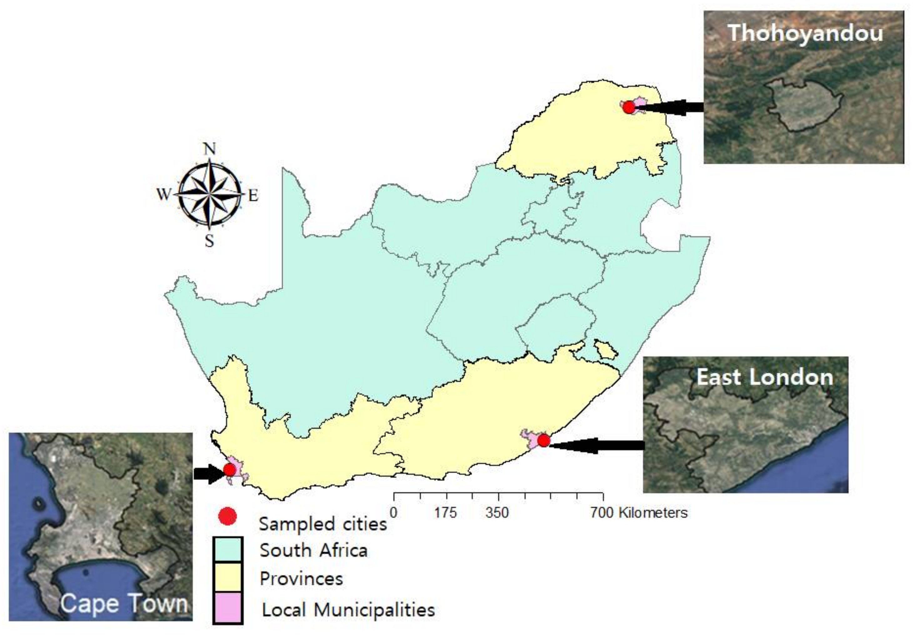
The study was conducted in Cape Town, Thohoyandou and East London urban areas of the Western Cape, Limpopo and Eastern Cape provinces of South Africa, respectively (Figure 1). These are urban areas of different size, urban form and land-use systems, representing a gradient across South African urbanization. Their geographical location and dispersion through South Africa put them in different climatological systems. Cape Town and East London are coastal cities, while Thohoyandou is a remote inland small town (Figure 1).
Cape Town, located at the southernmost tip of Africa, experiences a Mediterranean climate characterized by cold wet winters and hot dry summers [35]. East London experiences a maritime climate with cool winters and mild summers that is moist throughout the year because of proximity to the ocean [36]. Thohoyandou experiences cold dry winters and hot wet summers [37]. Cape Town as a city is a monument of the historical occupations and influences of the diverse people groups who contributed to its development. This has greatly influenced urban form resembling Portuguese, Indian, Dutch and British architecture [38]. The original development of Cape Town into somewhat of an urban area began with the Portuguese explorers in the 14th century in an area that belonged to the Khoikhoi people. This was followed by the Dutch period in the 17th century and then the British period in the 19th century. Finally, the South African period began in the early 20th century and extends to date. The 20th century ushered in rapid urban expansion in Cape Town from multiple epicenters, resulting in an overall design that is comprised of multiple administration and suburban residential areas resembling Harris and Ullman’s (1945) multiple nuclei model [39]. Cape Town currently sits at 400 km2 with a population density of 17,500 per km2.
East London similar to Cape Town was also developed originally as a harbor town. However, East London does not have as long a history of cultural diversity from different developers as cape town. The city has remained a harbor city of mostly British influence in style, but the expansion outwards into the indigenous communities has brought indigenous cultural influences into the East London urban form [40]. It is currently sitting at an area of 168.9 km2 and a population density of 2745 per km2.
Thohoyandou, which was developed as a capital for the Venda Bantustan in the latter half of the 20th century, does not benefit from the diversity of historical western influences in its urban form and design that East London and Cape Town encompasses [41]. The development of Thohoyandou was originally for a shopping center and government administration offices [42]. Among the three urban areas, Thohoyandou is the most integrated with features associated with the rural environment. The area of Thohoyandou is 42.62 km2 with a population density of 2051 per km2.
2.2. Materials and Methods
2.2.1. Sentinel-2 Multispectral Imagery
The Sentinel 2 Top-of-Atmosphere (ToA) (L1C) product was obtained from the Copernicus Open Access Hub (COAH) of the European Space Agency (ESA). Sen2Cor288 algorithm was used in SNAP to correct for atmospheric interference and thus convert the L1C product to Sentinel L2A, which is Bottom-of-Atmosphere (BoA) reflectance [43]. Sen2Cor creates BoA reflectance images, terrain and cirrus corrected reflectance, aerosol optical thickness, water vapor, scene classification maps and quality indicators for cloud and snow probabilities [44]. The central month image of each season with a cloud coverage filter of less than 0.5% was selected as the most suitable to reflect peak season dynamics (Table 1).
2.2.2. Definition of LCZ Classification
The standard [15] LCZ classification framework was selected for this study to be applied across all three urban areas. A remote sensing-based approach was chosen over a GIS-based approach. A GIS approach to classification would require manual digitization of the entire image, which is laborious and time consuming. The processing of remotely sensed data also requires the manipulation and interpretation of digital data [45]. This tends to be a mathematically complex process due to the heterogeneity of materials and geometry of the features [46]. However, the advantage of the remote sensing-based route is that it can be automated. The irregularities of the geometry of the local climate zones becomes a challenge to both pixel and object-based classifications [45,47,48]. A pixel-based classification which was adopted for this study overcomes this geometric non-uniformity challenge by assigning every pixel into a single class based on the reflectance value [49].
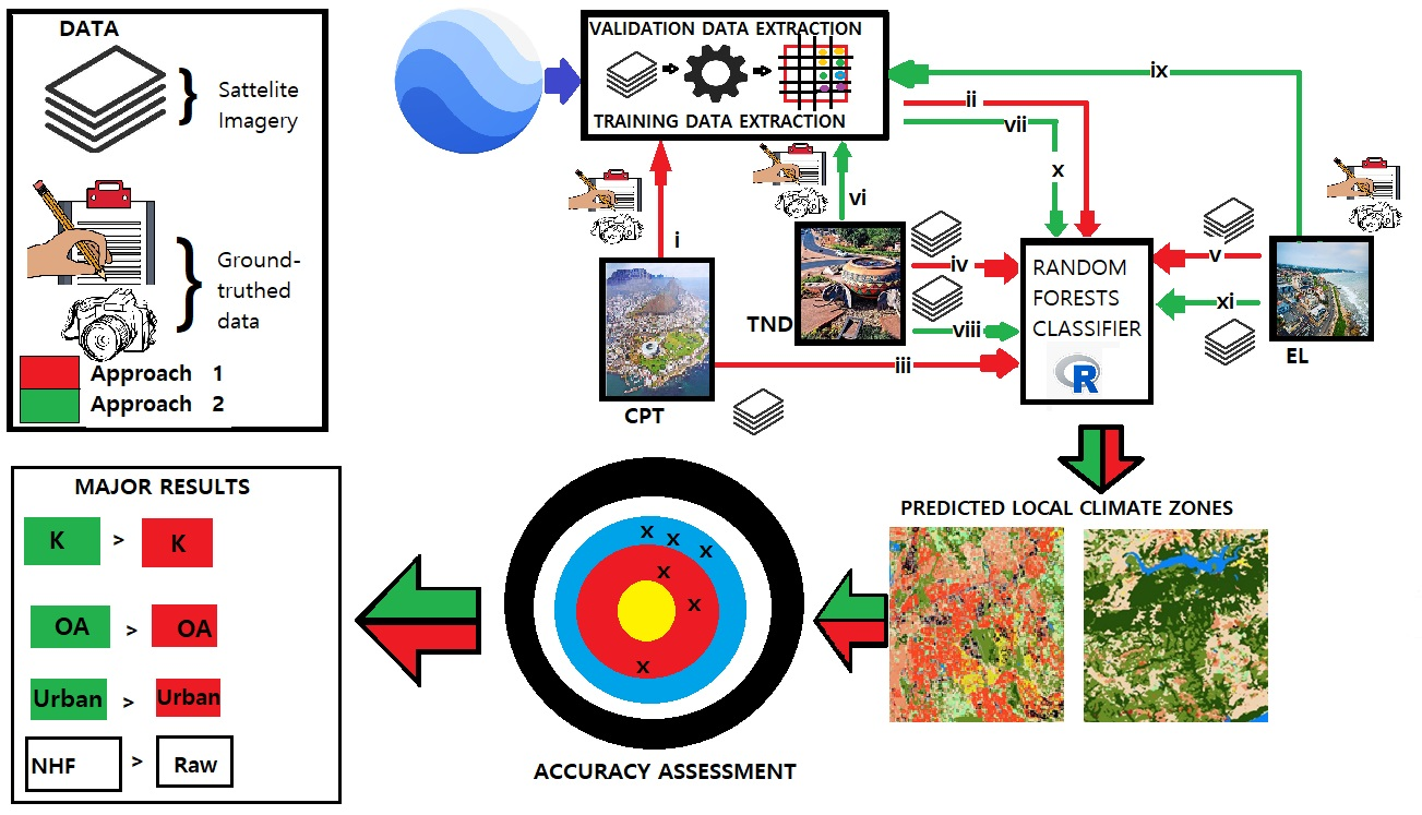
This application of Stewart and Oke’s LCZ classification framework was used in two approaches that differ in the creation of training data. Approach 1 followed strictly the LCZ region of interest (RoI) creation as outlined by WUDAPT to create a standard training set based on Cape Town to be applied on all three cities. The application of this remote training on Thohoyandou and East London indirectly assesses whether the influence of origin and culture on urban form affects the LCZ classification. This informs whether there is a need to have a customized training for LCZ classification in South African cities for all cities or locally for each urban region. Cape Town was chosen because it is the only urban area of the three that experiences all four seasons and contains all 17 LCZ standard classes [50]. Theoretically, this means that the impacts of phenology would be more apparent in Cape Town than in East London and Thohoyandou, which also would make it ideal for identifying the best season for single image classification across all three urban regions. In defining these LCZ classes, a separability analysis was performed. A spectral separability is an assessment of the performance of the Sentinel-2A multispectral instrument bands to differentiate between the classes of the typology. For the purposes of this study, histograms, scatter and box plots were used to perform this separability according to guidelines from [51]. The second approach to the classification still took off from the traditional [15] typology but explored combinations and subclasses of the standard typology based on the unique features of each urban region.
- i.
- Model TrainingTwo types of model training sets were developed for the classification where the first was standardized and the second was customized to the context of the urban area. The ground reference data were collected initially using digital globe resources due to COVID restrictions and were validated and revised in situ on February and March 2022 in Cape Town, Thohoyandou and East London. Based on a digital globe basemap, circular regions of interest were made using QGIS having a diameter of 100 m following the specifications of the standard typology as outlined by WUDAPT. The field campaign was then used as a manual method to verify the regions of interest (Figure 2). Most (80%) of the regions of interest were used for training and the remaining 20% were used for validation. The field campaign was also used to observe and document the unique elements of each urban region for the discriminations of subclasses to feed into the more specific training for Approach 2.
- a.
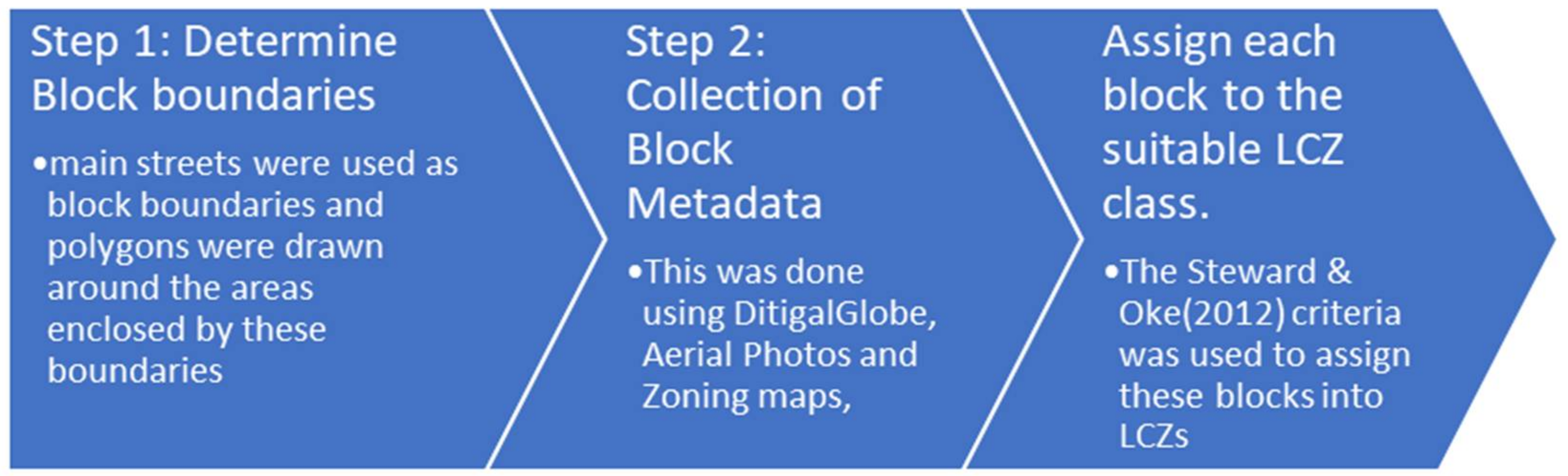
- Approach 1The WUDAPT LCZ typology guidelines for the development of training data was applied. These guidelines are divided into subcategories depending on the scale of the total area, classification methods and the intended use of the final product [47]. These guidelines have a strict protocol for training with the objective of using the WUDAPT online LCZ generator as well as a more flexible protocol for developing training data to be used outside the WUDAPT generator [16]. The development of these training polygons depends on a combination of general typology elements such as cover, material, geometry and function taken to different levels of detail depending on the scale of the imagery and the purpose of the classification. Cities are then mapped using the scheme of [15], which classifies the urban landscape into 10 urban and seven natural classes. Each class in the typology represents a LCZ described in terms of specific landscape parameters of mean building height, canyon width, aspect ratio, building surface ratio and impervious area. These training areas are used to characterize the reflectance properties of each LCZ, which is then used to develop a model that assigns every other untrained pixel of the image into the LCZ classes within the framework.A three-step sampling method (Figure 3) was adopted from [52]. This block-based system was developed for LCZ classification at the city block scale primarily as GIS-based. In this study, this method was used to guide the development of training samples following the three steps.The natural city blocks are easier to assign to LCZ classes because they are homogenous, but the urban classes are much harder even with the physical access to the area. Urban LCZ metadata variables were thus limited to mean building height (), which is the number of stories as collected in the field, mean building height (BH), canyon width (CW), aspect ratio, building surface ratio and impervious area (Figure 4). When the number of stories per building is less than 10, every story is assumed to be 3 m; otherwise, Equation (1) is used for buildings with more than 10 stories [53]. Buildings with one to three stories were considered low-rise, four to nine stories were considered mid-rise, and more than nine stories were classified as high rise (Figure 5). Canyon width is estimated by the average distance between two buildings. Aspect ratio is estimated by the ratio of the building height (BH) to the canyon width (W). Building surface fraction (BSF) and impervious surface fraction (ISF) were estimated using simple calculations in QGIS following the polygonization method (Figure 4) for areas of built and impervious surfaces. These variables were all used to assign each one of the blocks into LCZ classes (Figure 5). Within each block, multiple points were placed at a distance of 200 m from each other. A circular buffer of 50 m was created around each point, ultimately becoming the circular LCZ training polygon. Each of these training polygons was at least 100 m from the next one. A total of 200 training polygons were selected for the model training.Building Height (BH) = H_(s) × 3.5 + 9.6 + 2.6 × (H_(s)/25): H_(s)
- b.
- Local Customized Training Input (Approach 2)This approach is developed based on the layout and design of each city taking into account features that are common across all three cities and features that are unique to the specific urban region. In Thohoyandou, the urbanized city center and the immediate blocks around the city center have rural features integrated into the urban landscape. The intra-block streets in Thohoyandou are not homogenous in material; some are asphalted while some are gravel. While in a standard framework, the building density and height stand out as the main discriminators for local climate zones, the street canyon material stands out just as significantly in Thohoyandou. This is also noted by [27], who stated that as a unique general feature, remote African urban areas tend to have more bare soils than western urban. While this might not be statistically significant for a highly urbanized and highly westernized city such as Cape Town, its significance in a small town such as Thohoyandou cannot be neglected without investigation. However, spectrally separating bare soil from impervious surfaces in a remote sensing approach at the level of the pixel (10 m) has inherent confusion in spectral signatures [54]. Therefore, Following Jin’s blocking, a GIS approach was developed in order to create a criterion for separating blocks that are completely asphalted from blocks that are gravel within the urban area without the inherent confusion of a remote sensing approach. A digitization process was applied to digital globe imagery to create asphalted and bare soil inter-street blocks (Figure 6).The output of this digitization was used to separate training inputs that are in gravel blocks from those that are in asphalted blocks. LCZ 3 was the only class observed to be present in both block types. The buildings within LCZ 9 in Thohoyandou are also further apart than they are in Cape Town and East London. The space between houses is thus confused with Shrublands (LCZ 14) due to the dry nature of the shrublands in Thohoyandou. In order to reduce this confusion, the low plants were thus combined with shrubs lands to form a single class. Scattered trees were also combined with dense trees to form a single class. The number of the natural classes was thus minimized so that the built classes can then stand out more spectrally. Impervious surface and bare soil were also combined to form a single class. This is because they are the least represented classes in the area, and combining them makes them a slightly larger class. This thus makes the updated training set for Thohoyandou to become LCZ 3a, 3b, 6, 8, 9, 11 & 12, 13 & 14, 15 & 16, 17.In East London, the ground truthing process in lightweight zones (LCZ 7) revealed a unique class that is a hybrid between lightweight and compact low-rise (Figure 7). A unique feature of South African light weight squatter camps is that they have no designated stand-numbers. This means they have no yards, and it is common for houses to share walls with their neighbors on all sides except the front. Because of this nature of South African squatter camps, the integration of LCZ 3 and LCZ 7 in these East London zones happens below the minimum size of the local climate (100 m). This is thus treated as a unique class and incorporated as LCZ 7a into the updated East London training, which then becomes LCZ 2, 3, 5, 6, 7, 7a, 8, 9, 10, 11, 13, 14, 16, 17.
- ii.
- Remote Sensing Classification ProtocolThe choice of the LCZ classification method is guided by the nature of the data, the available computational resources and the application purpose [45]. The classification protocol was performed via a coded script in R on R-Studio using mainly the CARET package through a Random Forests (RF) classifier. This was designed to extract the training pixels from the image stack, build predictive models that assign the rest of the image pixels into the most fitting class based on surface reflectance values and to validate the assigned pixels. This was performed on a single image stack as well as a multitemporal image stack.
- a.
- Single Image vs. Multitemporal Classification and Neighborhood FunctionThe first classification method is the most straightforward application of a LCZ classification and consists of applying the iterative process on a single date image. The seasonality was therefore analyzed in terms of meteorological seasons, namely winter, spring, summer and autumn, each in turn, by one scene at the center of the season [55]. For the multitemporal approach, accuracies of single-image classifications of each season will therefore be compared with those of a classification combining images of all four seasons. This is in order to account for the spectral and spatial changes in the natural vegetation that is caused by seasonal changes. This has the potential to increase the accuracy of the classification. This eliminates confusing between seasonal classes such as bare soil in the dry period, which is covered by low vegetation in the rainy periods.
- b.
- Neighborhood FunctionA neighborhood function or contextual classifier can contribute to increased accuracies in the classification of urban areas that are internally highly differentiated or heterogeneous, resulting from historical urbanization patterns that reflect the locality and the culture. In addition, most classification methods, including the original WUDAPT protocol, do not take this spatial variation into account. Moreover, the WUDAPT workflow causes a loss of spectral variability information before the actual classification by resampling the Landsat images during the pre-processing phase to a spatial resolution of 100 m [56,57,58,59,60]. At 10 m resolution, the sensitivity of the neighborhood function was tested by increasing the size of the kernel window for an optimal cell number.
- iii.
- ValidationThe ground truth data were randomly split in R into a training (80%) and validation (20%) set. The validation set is used to validate the model using accuracy metrics. The first accuracy metric performed was visual comparison of the output with satellite imagery. The User Accuracy (UA) is the probability that the predicted value is correct; the Producer’s Accuracy (PA) is the probability that a value in a certain class was classified correctly. The Overall Accuracy (OA), the Kappa coefficient, is a measure of the agreement between classification and truth values. All were calculated according to the guidelines in [48]. The F1-score was calculated as the harmonic mean of the UA and PA, which is even more useful when the classes are not balanced.
3. Results
3.1. Local and Remote Standard LCZ Training (Approach 1)
3.1.1. Visual Analysis of the Classification Outputs
A visual inspection of the Cape Town output reveals a clear separation of the built from the natural classes (Figure 8). What this pattern also reveals is that the compact classes are rather concentrated next to each other and the open classes are further away. The city center toward the harbor is composed of compact high-rises and compact mid-rises, as expected in a modern city such as Cape Town. The agricultural lands up north are also visible from a visual inspection with minor patches of LCZ 9 through them. What is also worth noting is the confusion that arises between the paved surfaces and built classes. Roads at the city center are wrongfully classified as either compact high-rise (LCZ 1) or heavy industry (LCZ 10).
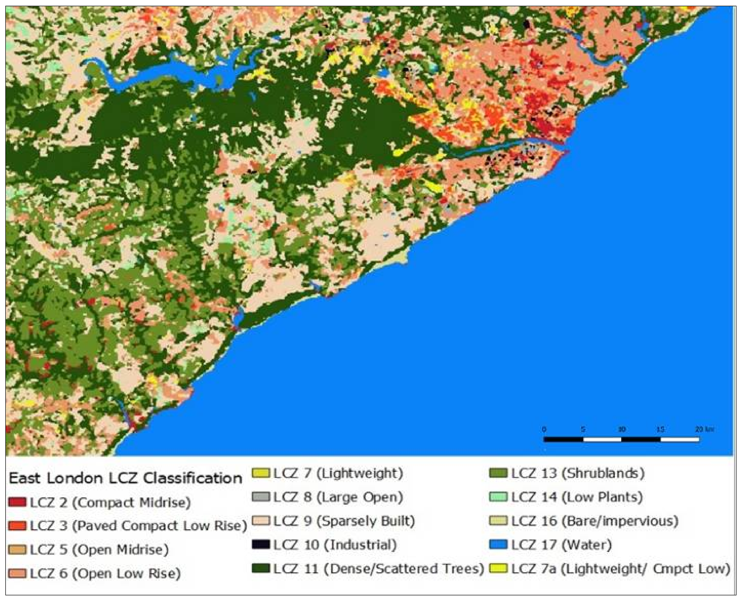
When the remote Cape Town-based standardized training is applied on a Thohoyandou multitemporal image, LCZ 3 is completely absent (Figure 9A), but it reappears immediately when a local standardized training is applied (Figure 9B). Using a local standardized training shows the Nandoni area to be mostly LCZ 9 with some vegetation; this is in line with the pre-study survey and google globe imagery that show the area being a rural village. However, the remote standardized training shows the same area as being mostly composed of LCZ 8 (Large Open), which is mostly found in the city center. Single-image classification using remote training shows LCZ 7 (light low-rise) at the city center, which according to google globe is a misclassification, as Thohoyandou does not have squatter camps, and this remote training also shows forested environment at the Nandoni region. This is different from the output of the local training, which is almost in complete agreement with the local MT classification showing no LCZ 7 at the city center and low plants and sparse trees at the Nandoni dam area. The application of remote vs. local training in East London does not yield significant differences in the appearance of classification outputs.
3.1.2. Single Versus Multi-Seasonal Images and Neighborhood Functions Comparing Performance of Remote and Local Standard Trainings
While the multitemporal Cape Town image is the most accurately classified with an overall accuracy of 44%, the spring image has the highest accuracy of the single image classifications with an accuracy of 42% (Table 2). The difference in Kappa and OA metrics between the spring image and the multitemporal image is relatively small: 1.6% for Kappa and 1.4% for OA. This suggests that the spring image could be an acceptable representation of the Cape Town area when there are no multitemporal data. The spring image OA is a 6% improvement on the summer classification, which is at 36%. However, even this 6% is mostly due to the natural vegetation (OA-nat), which is 15% higher in spring than in the summer. The difference between accuracies of the urban classes (OA-urb) is only 2%. This also proves that the effects of phenology are greatest among natural classes, as expected. The summer image as the least successfully classified has the lowest Kappa at 31.2%, which is a 68.8% disagreement between the training and the output. This indicates that the least represented classes in the training are not very well classified. According to the Kappa statistic, the least classified (summer) and the best classified (multitemporal) all have Kappa values that fall within the same range. This means about 60% disagreement between training and output, suggesting that only 40% of the data can be relied upon to produce the observed results. The difference between the F1 score and the OA is also Indicative of patterns in classification of individual classes, since the F1 is a harmonic mean of the PA and UA. From Table 2, the summer and autumn images F1-scores and OA are almost identical which indicates confusion even in the classes which are rather well classified in other seasons.
The confusion matrix of the spring image shows that the built classes have more confusion than the natural classes (Table 3). While LCZ 3 and LCZ 6 are visually well represented across all reasons, the confusion matrix reveals that they have the highest confusion in general. A lot of bare lands in the summer and autumn are classified as built classes. This trend is also seen in the spring season with LCZ 16 confused with LCZ 9 and LCZ 10. However, the spring image is still the best classified single date image and is the best season to test the Cape Town based remote training in Thohoyandou and East London. The other tool that improves the classification is the contextual classifier, and the optimal kernel size must be determined for application across all urban areas. This fragmentation (salt and pepper effect) of classes is most visible from the classification output (Figure 8 and Figure 9).
The neighborhood function aggregates the pixels within a certain threshold into a single value and results in a smoother output as compared to the raw data classification (Figure 10). This is tested on Cape Town and the optimal kernel size applied to Thohoyandou and East London to compare their results with Cape Town. The accuracy remains constant at 42.7% and Kappa at 43.2% for all kernel sizes below 11 cells and reaches its peak at 13 cells, after which the accuracy starts to decrease (Table 4).
With a 13 × 13 kernel of 130 m at a resolution of 10 m, the accuracy of the spring single image classification is improved by 6.0%, and the multitemporal classification is improved by 5.7%. However, in general, the multitemporal combined with the neighborhood function still yields higher accuracies than the single image with the neighborhood function. The highest overall accuracy of the multitemporal is 49.8% at a 13 × 13 moving window size, bringing the total improvement over the general single image to 7.2%.
Nevertheless, it is only a slight improvement of 1.1% compared to the single-image classification, which has an overall accuracy of 47.7%. Table 5 also shows that for both the single and multitemporal classifications, the overall accuracy of the combinations of both natural and built classes (OA-nat/urb) metric is highest at a kernel size of 11 × 11 or 110 m, indicating that confusion between natural classes and built classes is lower in these classifications. However, this is only a 0.3% difference from the 13-cell kernel application, which individually has higher OA-nat and OA-urb. For the purposes of this classification, a standard 13 cell NH kernel was adopted as the optimal kernel size for comparison across the three urban regions.
The application of remote training yields the highest results in a Thohoyandou multi-date stack at 53.2%; however, a local standardized training yields a 7% increase in overall accuracy and a 10% increase in Kappa. Urban classes are less successfully classified across the board. However, they are better classified in East London than they are in Thohoyandou. The use of remote vs. local classification in East London does not seem to have as big an impact as it does on Thohoyandou. The multi-date classification using local standardized training is only 2.1% higher than its remote training counterpart. The single-date classification using remote training yields the lowest overall accuracy, Kappa and F1-metric across the board, while the multi-date local training yields the highest values of the same metrics. There seems to be a similarity in the LCZ layout between Cape Town and East London, which is seen through the accuracy metrics, which are almost similar for both remote and local training.
3.2. Classification Using Local Customized Training Data (Approach 2)
3.2.1. Thohoyandou Classification
- a.
- Random Splitting of Training Data
Using a randomized selection of training and test sample makes the model more robust, but it does not create an even number of pixels throughout. The challenge even in the development of the original training protocol was that some classes had better representation than others. While this can be avoided by creating an even amount of training samples throughout, there simply is not always enough land area to create regions of interest in some classes. Other classes also call for a higher number of training due to their inter-class variability that must be accounted for in the training sample. The output of the randomly selected training pixels (Figure 11A) shows that classes 14, 15 and 16 do not have enough representation in the sample. This was solved by joining them to other classes that have similar spectral signatures. Class 14 was combined with class 13; class 15 was combined with class 16. The result of this ends up with the lowest number of pixels in the training going from 250 pixels to above 700 (Figure 11B).
- b.
- Single Versus Multi-Seasonal Classification and Comparison with Standard Training
What has been observed in Approach 1 classifications is still maintained in the Approach 2 results. This is the observation that the spring image provides the highest accuracy of all the single image classifications (Table 6). However, natural vegetation is more accurately classified in the winter NH than in any other season, while urban is highest in the spring. The multitemporal image that combines all the seasons is the most accurately classified with an accuracy of 82.68% as compared to 53.2% of Approach 1.
What the confusion matrix of the multitemporal classification reveals is that all the classes are more accurately classified than misclassified except for LCZ 16, which is a compound class of LCZ 15 and original LCZ 16. The highest confusion of LCZ 16 is with LCZ 8, which is due to the paved spaces between large open buildings, and LCZ 13, which is due to the large bare regions in between shrubs (Table 7).
The analysis of the multitemporal classification model reveals that the higher bands (Band 9—11) of each season are the most important in classifying the pixels (Figure 12). These are the SWIR (shortwave infrared) bands of the Sentinel 2A image stack.
The discrimination between the gravel LCZ 3a and the asphalted LCZ 3 seems to be very good according to a visual inspection of the classification output (Figure 13). The confusion matrix also confirms this with 17% of the LCZ 3 classified as LCZ 3a. However, the highest confusion with LCZ 3a is with LCZ 6. This is due to them sharing similar open spaces and also their proximity with 11.5% of LCZ 3a pixels classified as LCZ 6.
3.2.2. East London Classification
Using a local and customized training input yielded higher overall accuracy and Kappa values. The highest OA value for East London using Approach 1 was 41.3%, which has increased to 58.5% using Approach 2 which is a 17.5% increase. However, contrary to observations from the Approach 1 results, the multitemporal image does not appear to be the best fit for both built and natural classes. The spring image with a 13-cell neighborhood function yields the highest overall Kappa, F1-Score, and overall accuracy (Table 8). This is in agreement with the observation made in Approach 1, where the spring image was the highest of the seasonal single image classifications. What is also similar is that the summer image has the lowest values for all the overall metrics. It is worth noting that the spring image still has the highest number of lowest individual class Kappa values spread out across built classes; this suggests that the higher overall metrics are due to the perfect and near perfect classification of the natural classes. The highest individual LCZ Kappa values are not localized to a single season but spread out through different seasons. A common trend, however, is that the highest individual Kappa values fall within the classifications that have been smoothed out with the 13-cell kernel, while the lowest values are within the raw image classification.
What the spring neighborhood function image (Figure 14) reveals visually is that LCZ 7 and 7a are in close proximity to LCZ 3. This goes from a strict LCZ 3 and moves into LCZ 7a, which is an integration of 7 and 3, and then ultimately moves into a strict LCZ 7.
4. Conclusions
Cape Town is a multi-nuclei urban region of multi-cultural origin, East London is a harbor town, and Thohoyandou is a small town that originated as the administrative capital of the Venda Bantustan. These urban regions represent a gradient within urbanization in South Africa. These different historical backgrounds contribute to the uniqueness of the layout and feature type in each region, which is a phenomenon also noted in the Middle East [25]. These unique features become an element of importance, as they could potentially explain the poor performance of the standard framework when performed using multispectral imagery at the local scale in Africa. Cape Town as an urban area resembles closely the cities of the west; as such, the standard LCZ framework typology would best fit Cape Town with minimal to no adjustment in the guidelines for RoI creation. However, the development of a localized and customized training for East London and Thohoyandou individually creates a classification protocol that considers these unique local features stemming from influences of their unique origin and cultural evolution as they herd toward modernization.
The nature of the training input was the major difference between Approach 1 and Approach 2. Where Approach 1 used a single all-inclusive training input for all three cities, Approach 2 used a local customized training input for each urban region and yields better results. The biggest challenge in this study was the lack of a height layer in the stack as a discriminator for the algorithm. Ref. [61] stated that the presence of a height layer is essential for cities with LCZs belonging to different height classes (low, mid and high-rise). What is immediately noticeable in the accuracies metrics is the big difference between values obtained in homogenous-height Thohoyandou across all LCZs and the heterogenous-height Cape Town and East London using both Approaches 1 and 2 (Table 6, Table 7 and Table 8). Without a height discriminator in the classification stack, there is inter-class confusion within the compact classes as well as the open ones (Table 3). Ref. [62] addressed the height challenge by using an abridged version of the LCZ classification that considers surface feature density but eliminates height altogether. While this land cover-based framework by [62] was also proven to explain trends in urban heat islands, the local scale suffers from detail loss. This compromise of detail over accuracy renders the output less useful and to some degree even unsuitable for local climate models. The best way to address the height data gap challenge while maintaining detail resolution remains using locally calibrated training as opposed to the [62] land cover approach.
Both approaches revealed that a local customized training sample is a better fit for the random forest LCZ classifier than using a standardized training input for all regions. This is seen through the classifier performance being better in Approach 2 as opposed to Approach 1. The literature would also dictate that seasonality would mostly affect natural LCZ classes because of plant phenology [63,64,65]. However, as seen in the metric tables (Table 3, Table 6 and Table 7), urban classes are also classified to varying degrees of accuracy at different seasons. While the higher short-ware infrared (SWIR) bands are always the most important in the automated LCZ discrimination protocol, the lower bands range from minimally important to completely negligible. Studies by [66,67] isolate the variations in band priority for different seasons as a function of the physical properties of surface features. This is not limited to biotic but also abiotic features such buildings. The multitemporal classification was the most accurately classified of all classifications. Ref. [68] stated that the effects of seasonality are addressed by taking a multitemporal stack which covers classing during all stages of annual variability. While the actual seasons are classified to varying degrees, the multitemporal local customized training would still be more representative of the LCZ classes than using a single image from any season.
The size of the pixel also determines the accuracy. As such, a contextual classifier (NF) significantly improves the accuracy of the model [69]. While applying a neighborhood function does not change the pixel of the image, it reduces the level of detail in the classification output. This is seen by visually looking at the raw data output (Figure 9) as compared to the NF output (Figure 12). The fragmentation is less apparent when the pixel size is higher than 100 m, as seen when the WUDAPT online generator is used [66]. The disadvantage is that classifying LCZ with a local-scale pixel size (100 m) reduces the level of detail that that would otherwise be found in using higher-resolution imagery, which in this study was 10 m. This is crucial while working with urban climate models. The challenge in using a contextual classifier is in finding a kernel size that balances detail, accuracy and aesthetic for the specific goal for which the classification is intended to be used. While for the purpose of this study, the aim of the NF was to achieve the highest accuracy, the nested algorithm is flexible enough to modify the kernel size should the purpose of the classification be different.
An application of these methods in future studies should consider using more training samples for the less represented classes. In addition, whether the accuracy in Thohoyandou would improve if a height discriminator is part of the protocol is worth exploring further. Height is definitely recommended as an important addition to the classification stack for East London, Cape Town or any other city with mid- and high-rise classes. The findings of this particular study as well as the methodological protocols would be recommended for adoption by any future study that aims at studying UHIs in the African context, particularly investigating the spatial correlation between the patterns that are observed in the UHIs with the underlying LCZ classification.
Author Contributions
Conceptualization, T.M. and J.T., B.S., B.V.; Data curation, T.M. and J.T.; Formal analysis, T.M. and J.T.; Funding acquisition, B.S., B.V. and N.N.; Methodology, T.M., J.T., B.S., B.V.; Software, T.M. and J.T.; Visualization, T.M. and J.T.; Writing—original draft, T.M.; Writing—review and editing, T.M., B.S., B.V. All authors have read and agreed to the published version of the manuscript.
Funding
This work was funded by VLIR-UOS, the Flemish University Council for University Development Cooperation through the ReSider project and the Flemish government funded SAF-ADAPT project. Funding number: 000000166183.
Data Availability Statement
Data are available on request from the authors.
Acknowledgments
I would like to acknowledge the help of Anna Van Eyck in collecting the validation data in Thohoyandou and Cape Town in February-March 2022.
Conflicts of Interest
The authors declare no conflict of interest. The funders had no role in the design of the study; in the collection, analyses, or interpretation of data; in the writing of the manuscript; or in the decision to publish the results.
References
- Adams, R.M. The origin of cities. Sci. Am. 1960, 203, 153–172. [Google Scholar] [CrossRef]
- Robinson, E.; Zahid, H.J.; Codding, B.F.; Haas, R.; Kelly, R.L. Spatiotemporal dynamics of prehistoric human population growth: Radiocarbon ‘dates as data’ and population ecology models. J. Archaeol. Sci. 2019, 101, 63–71. [Google Scholar]
- Pierson, W.A. Spatial Assessment of Urban Growth in Cities of the Decapolis; and the Implications for Modern Cities. Ph.D. Thesis, University of Arkansas, Fayetteville, AR, USA, 2021. [Google Scholar]
- Schaedel, R.P.; Hardoy, J.E.; Scott-Kinzer, N. (Eds.) Urbanization in the Americas from Its Beginning to the Present; Walter de Gruyter: Berlin, Germany, 2011. [Google Scholar]
- Chen, S.; Chen, B.; Feng, K.; Liu, Z.; Fromer, N.; Tan, X.; Alsaedi, A.; Hayat, T.; Weisz, H.; Schellnhuber, H.J.; et al. Physical and virtual carbon metabolism of global cities. Nat. Commun. 2020, 11, 182. [Google Scholar] [CrossRef] [PubMed]
- Balchin, W.G.V.; Pye, N. A micro-climatological investigation of bath and the surrounding district. Q. J. R. Meteorol. Soc. 1947, 73, 297–323. [Google Scholar] [CrossRef]
- Stewart, I.D. Why should urban heat island researchers study history? Urban. Clim. 2019, 30, 100484. [Google Scholar] [CrossRef]
- Lhotka, O.; Kyselý, J.; Farda, A. Climate change scenarios of heat waves in Central Europe and their uncertainties. Theor. Appl. Climatol. 2018, 131, 1043–1054. [Google Scholar] [CrossRef]
- Profiroiu, C.M.; Bodislav, D.A.; Burlacu, S.; Rădulescu, C.V. Challenges of sustainable urban development in the context of population Growth. Eur. J. Sustain. Dev. 2020, 9, 51. [Google Scholar] [CrossRef]
- Al-Thani, H.; Koç, M.; Isaifan, R.J. A review on the direct effect of particulate atmospheric pollution on materials and its mitigation for sustainable cities and societies. Environ. Sci. Pollut. Res. 2018, 25, 27839–27857. [Google Scholar] [CrossRef] [PubMed]
- Longo, S.; Montana, F.; Sanseverino, E.R. A review on optimization and cost-optimal methodologies in low-energy buildings design and environmental considerations. Sustain. Cities Soc. 2019, 45, 87–104. [Google Scholar] [CrossRef]
- Griffith, D.A.; Can, A. Spatial statistical/econometric versions of simple urban population density models. In Practical Handbook of Spatial Statistics; CRC Press: Boca Raton, FL, USA, 2020; pp. 231–249. [Google Scholar]
- Zhou, X.; Okaze, T.; Ren, C.; Cai, M.; Ishida, Y.; Watanabe, H.; Mochida, A. Evaluation of urban heat islands using local climate zones and the influence of sea-land breeze. Sustain. Cities Soc. 2020, 55, 102060. [Google Scholar] [CrossRef]
- Zhou, D.; Xiao, J.; Bonafoni, S.; Berger, C.; Deilami, K.; Zhou, Y.; Frolking, S.; Yao, R.; Qiao, Z.; Sobrino, J.A. Satellite remote sensing of surface urban heat islands: Progress, challenges, and perspectives. Remote Sens. 2019, 11, 48. [Google Scholar] [CrossRef] [Green Version]
- Stewart, I.D.; Oke, T.R. Local climate zones for urban temperature studies. Bull. Am. Meteorol. Soc. 2012, 93, 1879–1900. [Google Scholar] [CrossRef]
- Bechtel, B.; Alexander, P.J.; Böhner, J.; Ching, J.; Conrad, O.; Feddema, J.; Mills, G.; See, L.; Stewart, I. Mapping local climate zones for a worldwide database of the form and function of cities. ISPRS Int. J. Geo-Inf. 2015, 4, 199–219. [Google Scholar] [CrossRef] [Green Version]
- Mushore, T.D.; Mutanga, O.; Odindi, J. Determining the Influence of Long Term Urban Growth on Surface Urban Heat Islands Using Local Climate Zones and Intensity Analysis Techniques. Remote Sens. 2022, 14, 2060. [Google Scholar] [CrossRef]
- Yang, J.; Wang, Y.; Xiu, C.; Xiao, X.; Xia, J.; Jin, C. Optimizing local climate zones to mitigate urban heat island effect in human settlements. J. Clean. Prod. 2020, 275, 123767. [Google Scholar] [CrossRef]
- Zheng, Y.; Ren, C.; Xu, Y.; Wang, R.; Ho, J.; Lau, K.; Ng, E. GIS-based mapping of Local Climate Zone in the high-density city of Hong Kong. Urban. Clim. 2018, 24, 419–448. [Google Scholar] [CrossRef]
- Brousse, O.; Georganos, S.; Demuzere, M.; Vanhuysse, S.; Wouters, H.; Wolff, E.; Linard, C.; Nicole, P.M.; Dujardin, S. Using local climate zones in sub-Saharan Africa to tackle urban health issues. Urban. Clim. 2019, 27, 227–242. [Google Scholar] [CrossRef] [Green Version]
- Engelbrecht, C.J.; Engelbrecht, F.A. Shifts in Köppen-Geiger climate zones over southern Africa in relation to key global temperature goals. Theor. Appl. Climatol. 2016, 123, 247–261. [Google Scholar] [CrossRef]
- Wichmann, J. Heat effects of ambient apparent temperature on all-cause mortality in Cape Town, Durban and Johannesburg, South Africa: 2006–2010. Sci. Total Environ. 2017, 587, 266–272. [Google Scholar] [CrossRef] [Green Version]
- Kiet, A. Arab culture and urban form. Focus 2011, 8, 10. [Google Scholar] [CrossRef] [Green Version]
- Živković, J. Urban form and function. Clim. Action 2020, 862–871. [Google Scholar] [CrossRef]
- Saleh, M.A.E. The impact of Islamic and customary laws on urban form development in southwestern Saudi Arabia. Habitat Int. 1998, 22, 537–556. [Google Scholar] [CrossRef]
- Huang, J.; Lu, X.X.; Sellers, J.M. A global comparative analysis of urban form: Applying spatial metrics and remote sensing. Landsc. Urban Plan. 2007, 82, 184–197. [Google Scholar] [CrossRef]
- Akinyemi, F.O.; Ikanyeng, M.; Muro, J. Land cover change effects on land surface temperature trends in an African urbanizing dryland region. City Environ. Interact. 2019, 4, 100029. [Google Scholar] [CrossRef]
- Wang, R.; Ren, C.; Xu, Y.; Lau, K.K.L.; Shi, Y. Mapping the local climate zones of urban areas by GIS-based and WUDAPT methods: A case study of Hong Kong. Urban Clim. 2018, 24, 567–576. [Google Scholar] [CrossRef]
- Demuzere, M.; Kittner, J.; Bechtel, B. LCZ Generator: A web application to create Local Climate Zone maps. Front. Environ. Sci. 2021, 9, 637455. [Google Scholar] [CrossRef]
- Mushore, T.D.; Dube, T.; Manjowe, M.; Gumindoga, W.; Chemura, A.; Rousta, I.; Odindi, J.; Mutanga, O. Remotely sensed retrieval of Local Climate Zones and their linkages to land surface temperature in Harare metropolitan city, Zimbabwe. Urban Clim. 2019, 27, 259–271. [Google Scholar] [CrossRef]
- Lei, N.; Masanet, E. Climate-and technology-specific PUE and WUE estimations for US data centers using a hybrid statistical and thermodynamics-based approach. Resour. Conserv. Recycl. 2022, 182, 106323. [Google Scholar] [CrossRef]
- Dimitrov, S.; Popov, A.; Iliev, M. Mapping and Assessment of Urban Heat Island Effects in the City of SOFIA, Bulgaria Through Integrated Application of Remote Sensing, Unmanned Aerial Systems (UAS) and GIS. In Proceedings of the Eighth International Conference on Remote Sensing and Geoinformation of the Environment (RSCy2020), Paphos, Cyprus, 16–18 March 2020; International Society for Optics and Photonics: Bellingham, WA, USA, 2020; Volume 11524, p. 115241A. [Google Scholar]
- Zonato, A.; Martilli, A.; Di Sabatino, S.; Zardi, D.; Giovannini, L. Evaluating the performance of a novel WUDAPT averaging technique to define urban morphology with mesoscale models. Urban Clim. 2020, 31, 100584. [Google Scholar] [CrossRef]
- Rodríguez-Carrión, N.M.; Hunt, S.D.; Goenaga-Jimenez, M.A.; Vélez-Reyez, M. June. Determining optimum pixel size for classification. In Algorithms and Technologies for Multispectral, Hyperspectral, and Ultraspectral Imagery XX; International Society for Optics and Photonics: Bellingham, WA, USA, 2014; Volume 9088, p. 90880X. [Google Scholar]
- Pascale, S.; Kapnick, S.B.; Delworth, T.L.; Cooke, W.F. Increasing risk of another Cape Town “Day Zero” drought in the 21st century. Proc. Natl. Acad. Sci. USA 2020, 117, 29495–29503. [Google Scholar] [CrossRef]
- Van der Walt, A.J.; Fitchett, J.M. Statistical classification of South African seasonal divisions on the basis of daily temperature data. S. Afr. J. Sci. 2020, 116, 1–15. [Google Scholar] [CrossRef]
- Chikoore, H.; Bopape, M.J.M.; Ndarana, T.; Muofhe, T.P.; Gijben, M.; Munyai, R.B.; Manyanya, T.C.; Maisha, R. Synoptic structure of a sub-daily extreme precipitation and flood event in Thohoyandou, north-eastern South Africa. Weather Clim. Extrem. 2021, 33, 100327. [Google Scholar] [CrossRef]
- Worden, N.; Van Heyningen, E.; Bickford-Smith, V. Cape Town: The Making of a City: An Illustrated Social History; Uitgeverij Verloren: Hilversum, The Netherlands, 1998. [Google Scholar]
- Bickford-Smith, V. Creating a city of the tourist imagination: The case of Cape Town, The fairest Cape of them all’. Urban. Stud. 2009, 46, 1763–1785. [Google Scholar] [CrossRef]
- Thornberry, E. Rape, Race, and Respectability in a South African Port City: East London, 1870-1927. J. Urban. Hist. 2016, 42, 863–880. [Google Scholar] [CrossRef]
- Hangwelani, H.M.; Lovemore, C. The Impact of Island City in the Post-Apartheid South Africa: Focus on Bantustans. In Proceedings of the Urban Form and Social Context: From Traditions to Newest Demands, Krasnoyarsk, Russia, 5–9 July 2018; pp. 118–128. [Google Scholar]
- Kruger, J. Singing psalms with owls: A Venda twentieth century musical history. Afr. Music. J. Int. Libr. Afr. Music. 1999, 7, 122–146. [Google Scholar] [CrossRef] [Green Version]
- Sykas, D.; Papoutsis, I.; Zografakis, D. Sen4AgriNet: A Harmonized Multi-Country, Multi-Temporal Benchmark Dataset for Agricultural Earth Observation Machine Learning Applications. In Proceedings of the 2021 IEEE International Geoscience and Remote Sensing Symposium IGARSS, Brussels, Belgium, 11–16 July 2021; pp. 5830–5833. [Google Scholar]
- Main-Knorn, M.; Pflug, B.; Louis, J.; Debaecker, V.; Müller-Wilm, U.; Gascon, F. Sen2Cor for sentinel-2. Image Signal Process. Remote Sens. XXIII 2017, 10427, 37–48. [Google Scholar]
- Lillesand, T.; Kiefer, R.W.; Chipman, J. Remote Sensing and Image Interpretation; John Wiley & Sons: New York, NY, USA, 2015. [Google Scholar]
- Sekertekin, A.; Abdikan, S.; Marangoz, A.M. The acquisition of impervious surface area from LANDSAT 8 satellite sensor data using urban indices: A comparative analysis. Environ. Monit. Assess. 2018, 190, 1–13. [Google Scholar] [CrossRef]
- Bechtel, B.; Daneke, C. Classification of local climate zones based on multiple earth observation data. IEEE J. Sel. Top. Appl. Earth Obs. Remote Sens. 2012, 5, 1191–1202. [Google Scholar] [CrossRef]
- Foody, G.M. Status of land cover classification accuracy assessment. Remote Sens. Environ. 2002, 80, 185–201. [Google Scholar] [CrossRef]
- Weih, R.C.; Riggan, N.D. Object-based classification vs. pixel-based classification: Comparative importance of multi-resolution imagery. Int. Arch. Photogramm. Remote Sens. Spat. Inf. Sci. 2010, 38, C7. [Google Scholar]
- Tabi, K.A. Coping with Weather in Cape Town: Use, Adaptation & Challenges in an Informal Settlement. Master’s Thesis, University of the Western Cape, Cape Town, South Africa, 2013. [Google Scholar]
- Plantier, T.; Loureiro, M.; Marques, P.; Caetano, M. Spectral analyses and classification of ikonos images for forest cover characterisation. Cent. Remote Sens. Land Surf. 2006, 28, 260–268. [Google Scholar]
- Jin, L.; Pan, X.; Liu, L.; Liu, L.; Liu, J.; Gao, Y. Block-based local climate zone approach to urban climate maps using the UDC model. Build. Environ. 2020, 186, 107334. [Google Scholar] [CrossRef]
- Abrams, F. Mapping Local Climate Zones with SENTINEL Imagery in Ha Tinh and Hanoi, Vietnam; Katholieke Universiteit Leuven: Leuven, Belgium, 2019. [Google Scholar]
- Mora, C.; Vieira, G.; Pina, P.; Lousada, M.; Christiansen, H.H. Land cover classification using high-resolution aerial photography in adventdalen, Svalbard. Geogr. Ann. Ser. A Phys. Geogr. 2015, 97, 473–488. [Google Scholar] [CrossRef]
- Geletič, J.; Lehnert, M.; Savić, S.; Milošević, D. Inter-/intra-zonal seasonal variability of the surface urban heat island based on local climate zones in three central European cities. Build. Environ. 2019, 156, 21–32. [Google Scholar] [CrossRef]
- Bechtel, B.; Demuzere, M.; Mills, G.; Zhan, W.; Sismanidis, P.; Small, C.; Voogt, J. SUHI analysis using Local Climate Zones—A comparison of 50 cities. Urban. Clim. 2019, 28, 100451. [Google Scholar] [CrossRef]
- Demuzere, M.; Bechtel, B.; Middel, A.; Mills, G. Mapping Europe into local climate zones. PLoS ONE 2019, 14, e0214474. [Google Scholar] [CrossRef] [PubMed] [Green Version]
- Demuzere, M.; Hankey, S.; Mills, G.; Zhang, W.; Lu, T.; Bechtel, B. Combining expert and crowd-sourced training data to map urban form and functions for the continental US. Sci. Data 2020, 7, 264. [Google Scholar] [CrossRef]
- Van damme, S.; Demuzere, M.; Verdonck, M.L.; Zhang, Z.; Van Coillie, F. Revealing kunming’s (china) historical urban planning policies through local climate zones. Remote Sens. 2019, 11, 1731. [Google Scholar] [CrossRef] [Green Version]
- Verdonck, M.L.; Okujeni, A.; van der Linden, S.; Demuzere, M.; De Wulf, R.; Van Coillie, F. Influence of neighbourhood information on ‘Local Climate Zone’ mapping in heterogeneous cities. Int. J. Appl. Earth Obs. Geoinf. 2017, 62, 102–113. [Google Scholar] [CrossRef]
- Keany, E.; Bessardon, G.; Gleeson, E. Using machine learning to produce a cost-effective national building height map of Ireland to categorise local climate zones. Adv. Sci. Res. 2022, 19, 13–27. [Google Scholar] [CrossRef]
- Qiu, C.; Mou, L.; Schmitt, M.; Zhu, X.X. Local climate zone-based urban land cover classification from multi-seasonal Sentinel-2 images with a recurrent residual network. ISPRS J. Photogramm. Remote Sens. 2019, 154, 151–162. [Google Scholar] [CrossRef] [PubMed]
- Kabano, P.; Lindley, S.; Harris, A. Evidence of urban heat island impacts on the vegetation growing season length in a tropical city. Landsc. Urban Plan. 2021, 206, 103989. [Google Scholar] [CrossRef]
- Zhao, W.; Qu, Y.; Zhang, L.; Li, K. Spatial-aware SAR-optical time-series deep integration for crop phenology tracking. Remote Sens. Environ. 2022, 276, 113046. [Google Scholar] [CrossRef]
- Zhou, Y. Understanding urban plant phenology for sustainable cities and planet. Nat. Clim. Chang. 2022, 12, 302–304. [Google Scholar] [CrossRef]
- Cai, M.; Ren, C.; Xu, Y.; Lau, K.K.L.; Wang, R. Investigating the relationship between local climate zone and land surface temperature using an improved WUDAPT methodology—A case study of Yangtze River Delta, China. Urban. Clim. 2018, 24, 485–502. [Google Scholar] [CrossRef]
- Shi, L.; Ling, F.; Foody, G.M.; Yang, Z.; Liu, X.; Du, Y. Seasonal SUHI Analysis Using Local Climate Zone Classification: A Case Study of Wuhan, China. Int. J. Environ. Res. Public Health 2021, 18, 7242. [Google Scholar] [CrossRef]
- Rosentreter, J.; Hagensieker, R.; Waske, B. Towards large-scale mapping of local climate zones using multitemporal Sentinel 2 data and convolutional neural networks. Remote Sens. Environ. 2020, 237, 111472. [Google Scholar] [CrossRef]
- Yoo, C.; Han, D.; Im, J.; Bechtel, B. Comparison between convolutional neural networks and random forest for local climate zone classification in mega urban areas using Landsat images. ISPRS J. Photogramm. Remote Sens. 2019, 157, 155–170. [Google Scholar] [CrossRef]
Figure 1.
Geographic location of the Thohoyandou, East London and Cape Town relative to their respective municipalities, provinces and South Africa in general.
Figure 1.
Geographic location of the Thohoyandou, East London and Cape Town relative to their respective municipalities, provinces and South Africa in general.

Figure 2.
Some of the sampled locations across Cape Town, East London and Thohoyandou.
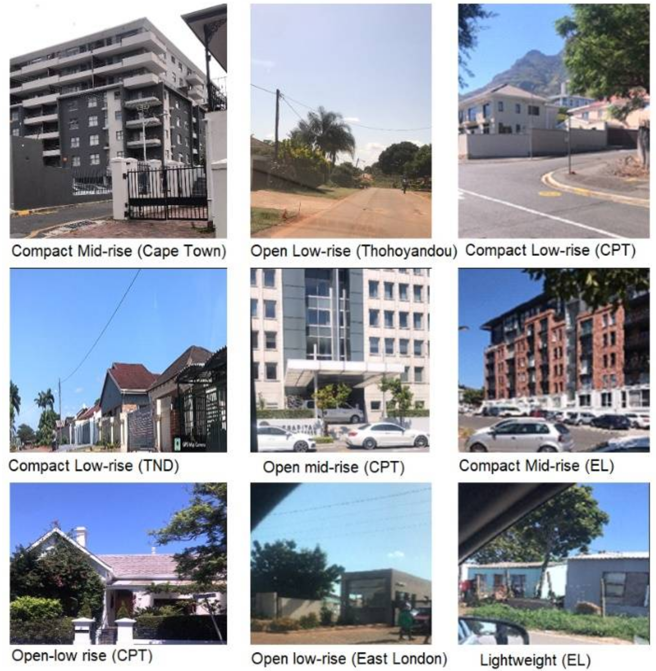
Figure 3.
An outline of the city block method steps for accurately creating training polygons and assigning them to different LCZ for the classification [15].
Figure 3.
An outline of the city block method steps for accurately creating training polygons and assigning them to different LCZ for the classification [15].

Figure 4.
A display of the method for mapping the features within each polygon in order to classify it to the suitable LCZ [53].
Figure 4.
A display of the method for mapping the features within each polygon in order to classify it to the suitable LCZ [53].
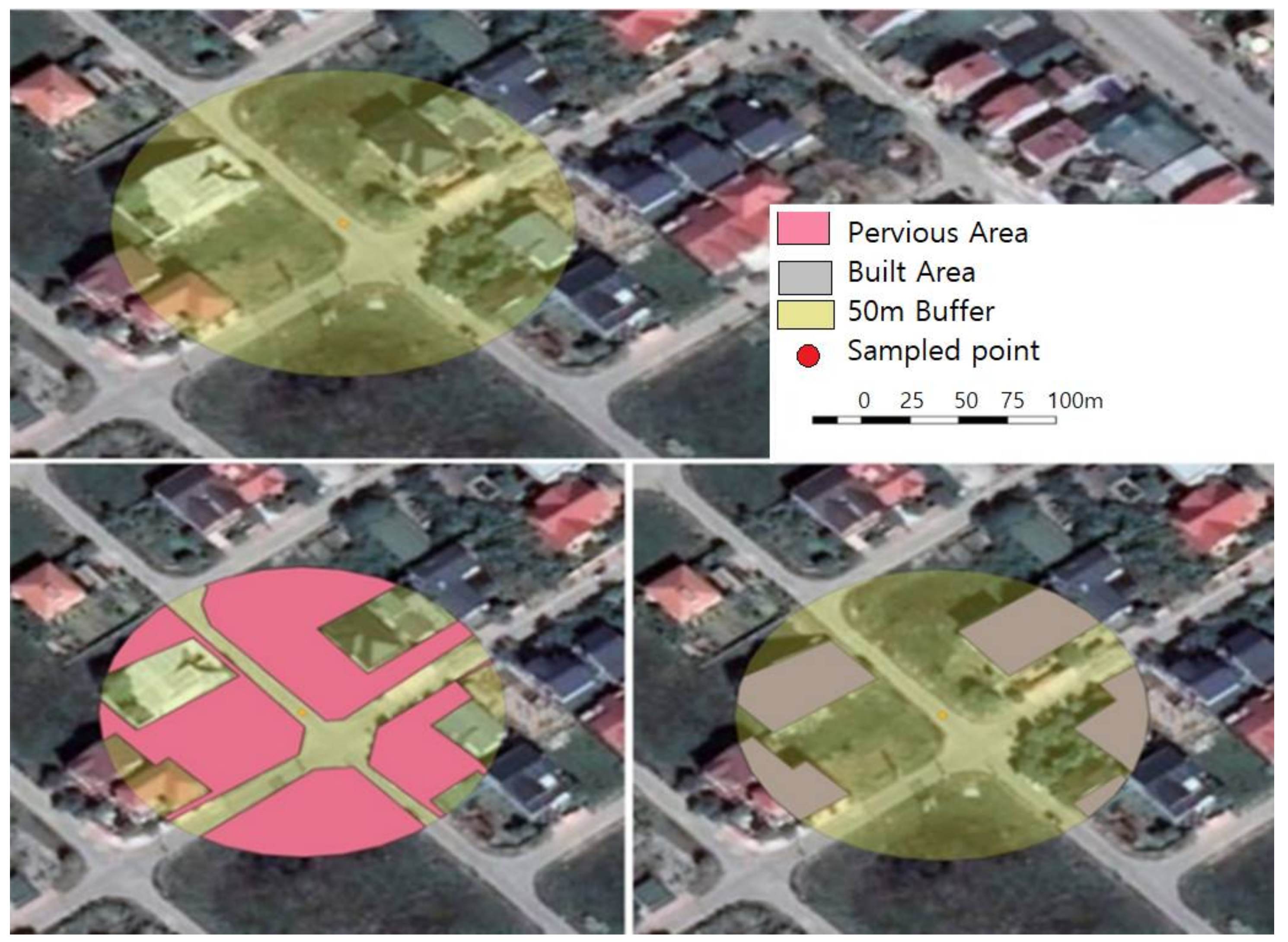
Figure 5.
A flow diagram of the final stage of the method for assigning training polygons to their suitable LCZ classes.
Figure 5.
A flow diagram of the final stage of the method for assigning training polygons to their suitable LCZ classes.

Figure 6.
Asphalted vs. bare soil (gravel) streets in Thohoyandou urbanized region.
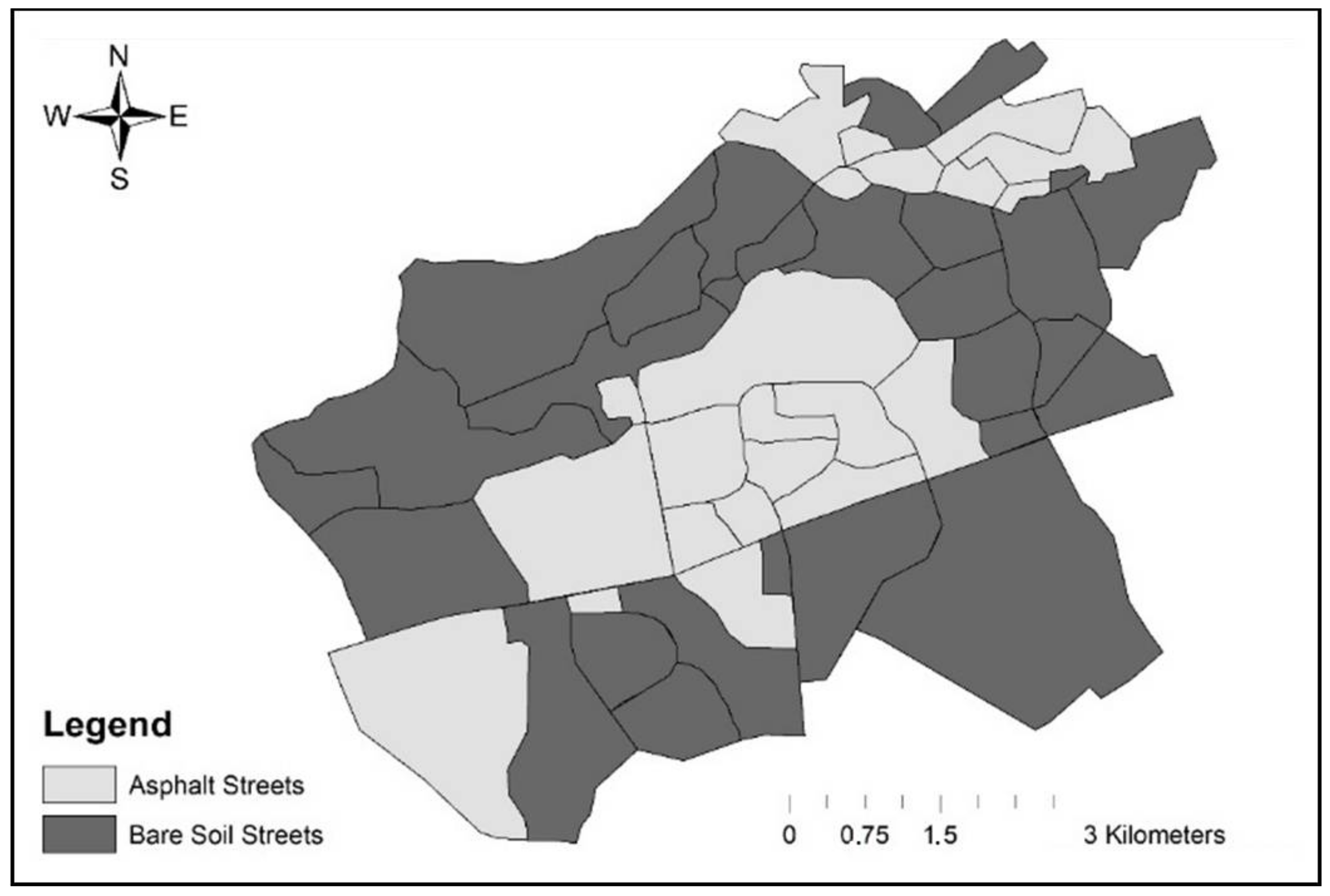
Figure 7.
East London squatter camp types; LCZ 7 showing a standard lightweight region while LCZ 7a shows a hybrid region of concrete and light weight.
Figure 7.
East London squatter camp types; LCZ 7 showing a standard lightweight region while LCZ 7a shows a hybrid region of concrete and light weight.
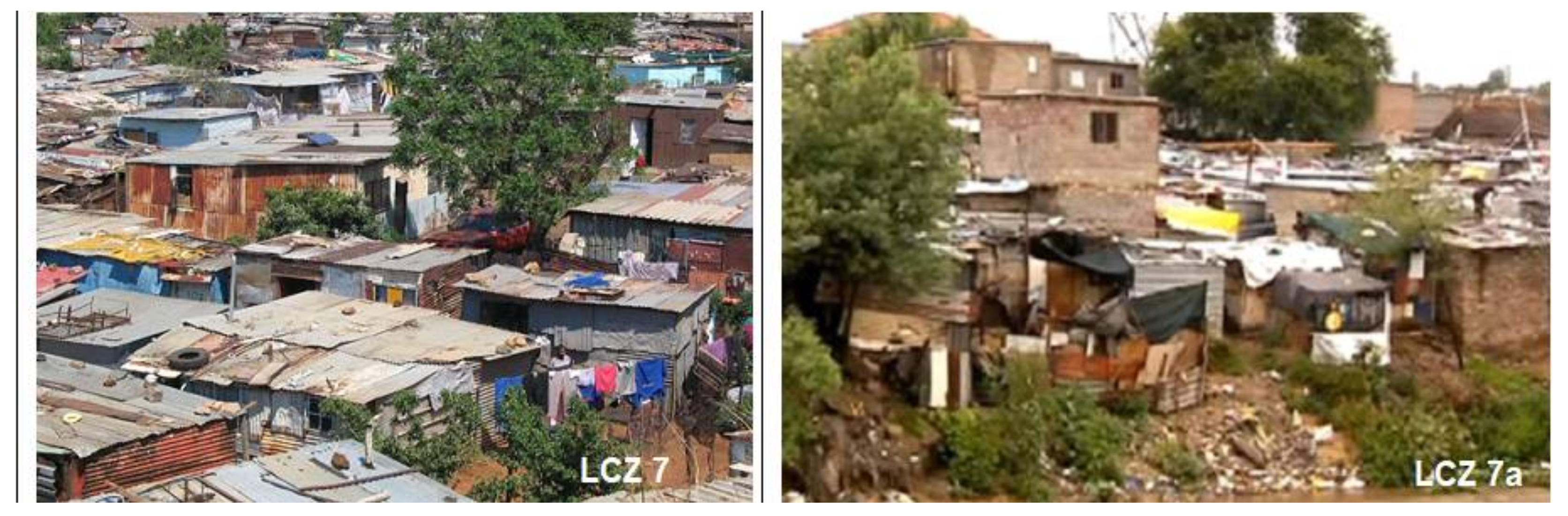
Figure 8.
Cape Town single image classifications across all 4 seasons with standard training according to WUDAPT guidelines.
Figure 8.
Cape Town single image classifications across all 4 seasons with standard training according to WUDAPT guidelines.
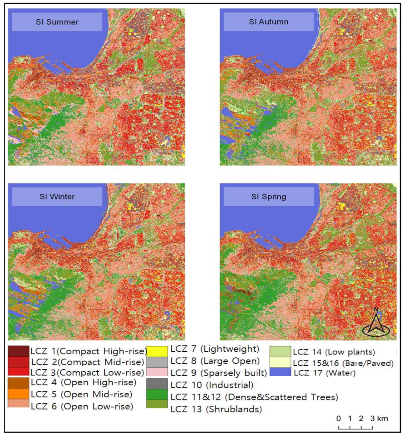
Figure 9.
Single image (C,D) and multi-temporal (A,B) classifications of Thohoyandou using a standardized remote (A,C) and local (B,D) training.
Figure 9.
Single image (C,D) and multi-temporal (A,B) classifications of Thohoyandou using a standardized remote (A,C) and local (B,D) training.

Figure 10.
Classification output for Cape Town with a neighborhood function of size 13.
Figure 11.
Pixels per class for the randomly selected training input for Approach 2 in Thohoyandou where (A) is unmerged and (B) is merged.
Figure 11.
Pixels per class for the randomly selected training input for Approach 2 in Thohoyandou where (A) is unmerged and (B) is merged.

Figure 12.
Band priority and importance in the class discrimination process for multitemporal stack in Thohoyandou.
Figure 12.
Band priority and importance in the class discrimination process for multitemporal stack in Thohoyandou.
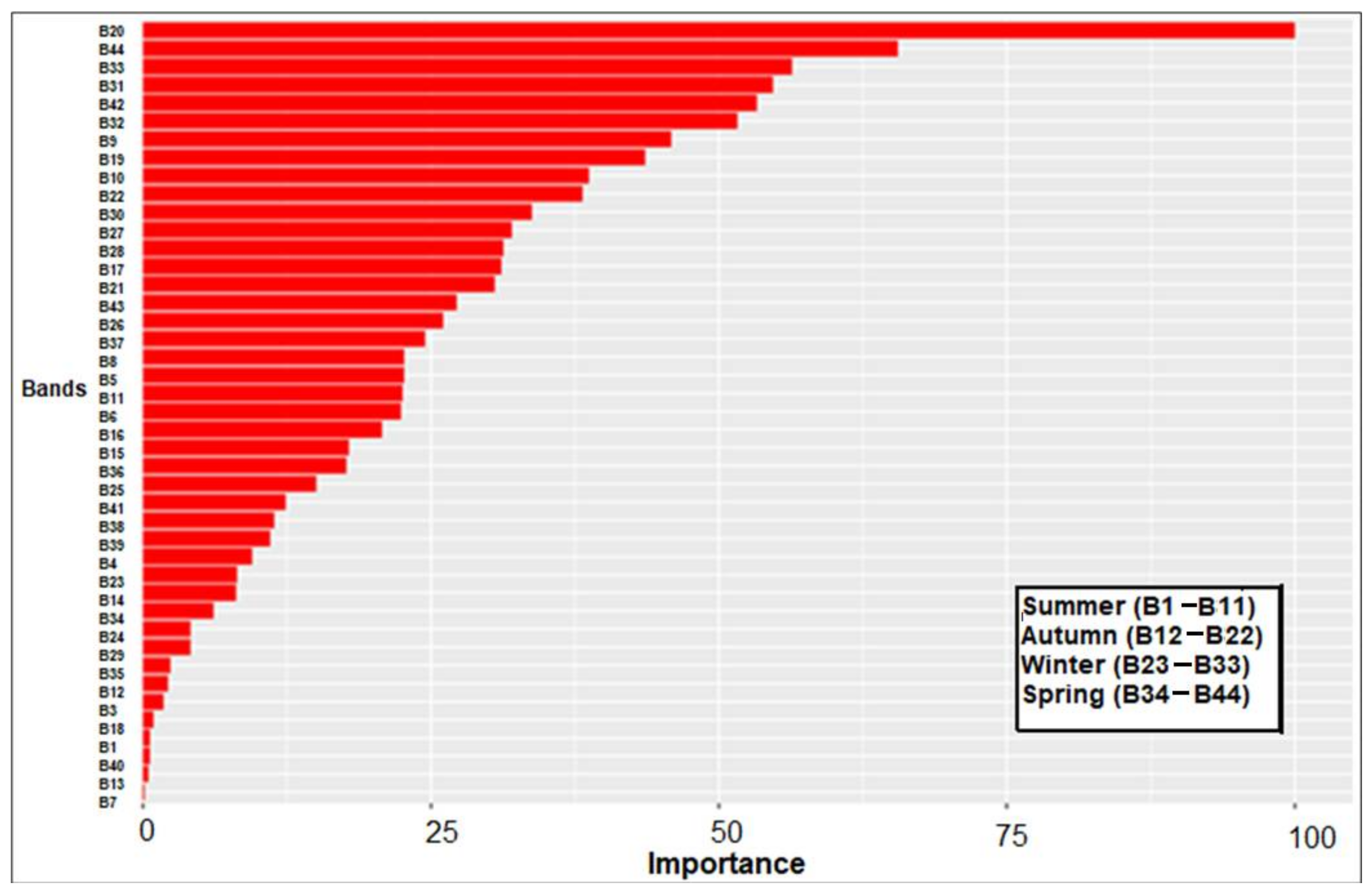
Figure 13.
Thohoyandou classification output for multitemporal with neighborhood function with local customized training showing asphalted and gravel streets.
Figure 13.
Thohoyandou classification output for multitemporal with neighborhood function with local customized training showing asphalted and gravel streets.
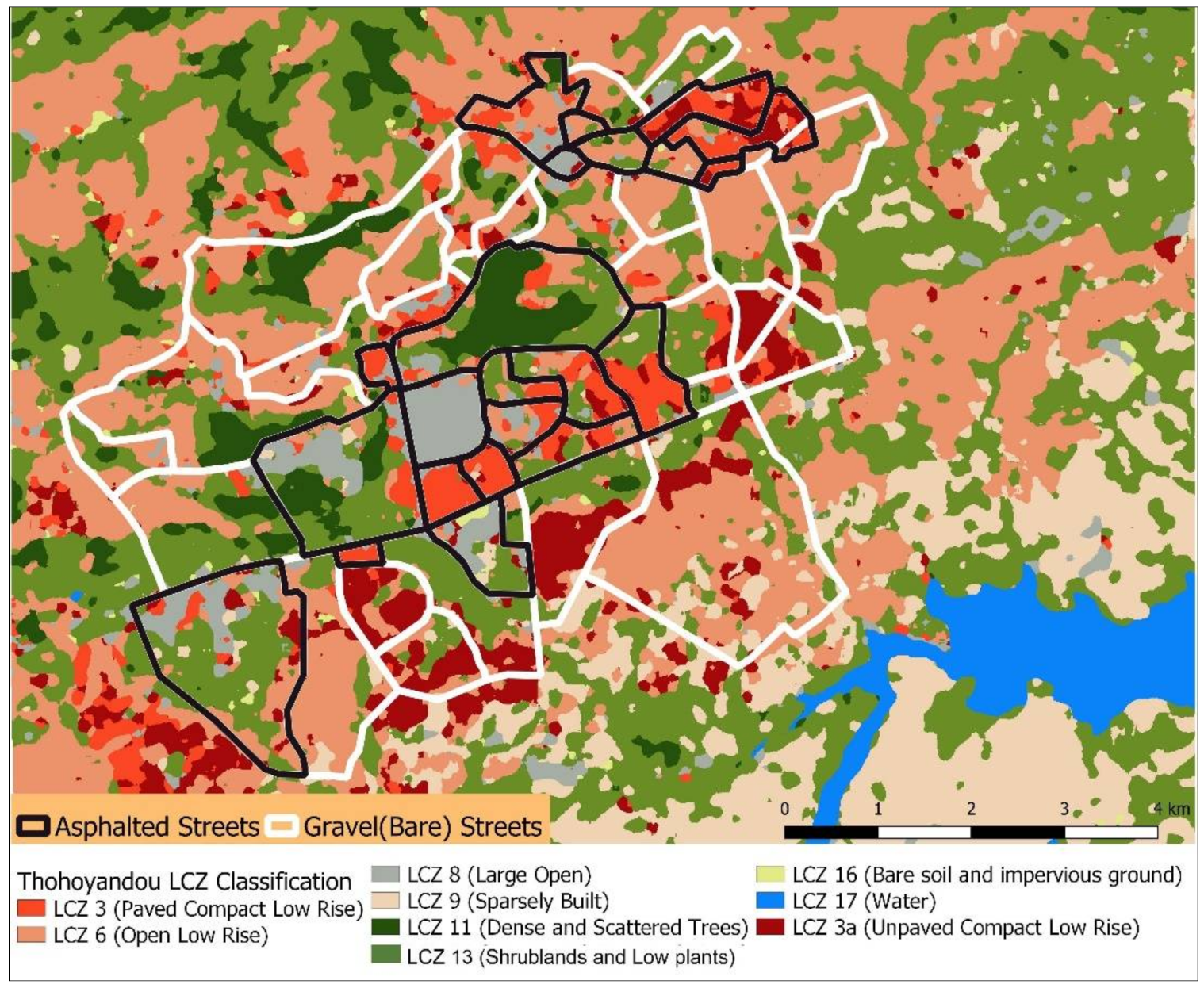
Figure 14.
East London classification output for multitemporal with neighborhood function using local customized training.
Figure 14.
East London classification output for multitemporal with neighborhood function using local customized training.

Table 1.
Date and seasons for the Sentinel-2 imagery used throughout the classification process.
| Sentinel-2 | ||||
|---|---|---|---|---|
| Summer | Autumn | Winter | Spring | |
| Cape Town | 25 February 2018 | 16 May 2018 | 24 August 2018 | 2 November 2018 |
| East London | 7 January 2018 | 28 March 2018 | 6 July 2018 | 14 September 2018 |
| Thohoyandou | 13 December 2018 | 27 April 2018 | 26 July 2018 | 24 September 2018 |
Table 2.
Accuracy metrics for single image and multitemporal random forest classifications over Cape Town.
Table 2.
Accuracy metrics for single image and multitemporal random forest classifications over Cape Town.
| Metrics | SI Summer | SI Autumn | SI Winter | SI Spring | Multitemporal |
|---|---|---|---|---|---|
| OA | 36.20% | 40.10% | 41.80% | 42.70% | 44.10% |
| OA-urb | 29.80% | 28.70% | 31.80% | 32.70% | 33.80% |
| OA-nat | 47.20% | 68.20% | 64.30% | 63.90% | 68.50% |
| Kappa | 31.20% | 35.50% | 37.20% | 38.00% | 39.60% |
| F1–metric | 36.50% | 40.40% | 42.60% | 43.20% | 45.20% |
Table 3.
Confusion matrix from the standard LCZ training single date spring image over Cape Town.
| Classified | Reference Classes | User’s Accuracy | ||||||||||||||
|---|---|---|---|---|---|---|---|---|---|---|---|---|---|---|---|---|
| 1 | 2 | 3 | 4 | 5 | 6 | 7 | 8 | 9 | 10 | 11 | 13 | 14 | 16 | 17 | ||
| 1 | 42 | 15 | 0 | 10 | 8 | 2 | 0 | 63 | 0 | 9 | 0 | 0 | 7 | 0 | 0 | 27% |
| 2 | 27 | 120 | 17 | 61 | 71 | 19 | 41 | 87 | 6 | 44 | 7 | 1 | 9 | 0 | 0 | 24% |
| 3 | 55 | 156 | 506 | 77 | 146 | 326 | 213 | 155 | 55 | 58 | 0 | 0 | 4 | 0 | 0 | 29% |
| 4 | 16 | 46 | 7 | 67 | 96 | 33 | 2 | 46 | 26 | 26 | 6 | 33 | 13 | 2 | 1 | 16% |
| 5 | 43 | 100 | 26 | 82 | 118 | 22 | 22 | 63 | 58 | 13 | 11 | 9 | 54 | 0 | 8 | 19% |
| 6 | 80 | 166 | 75 | 171 | 195 | 352 | 0 | 1 | 315 | 6 | 59 | 59 | 4 | 4 | 0 | 24% |
| 7 | 1 | 46 | 438 | 11 | 5 | 120 | 847 | 103 | 65 | 46 | 0 | 7 | 5 | 0 | 0 | 50% |
| 8 | 53 | 107 | 42 | 48 | 66 | 64 | 107 | 247 | 34 | 116 | 0 | 6 | 13 | 0 | 0 | 27% |
| 9 | 27 | 45 | 82 | 66 | 124 | 180 | 50 | 40 | 462 | 28 | 134 | 229 | 13 | 38 | 0 | 30% |
| 10 | 37 | 34 | 32 | 41 | 57 | 9 | 100 | 218 | 15 | 607 | 0 | 0 | 0 | 99 | 0 | 49% |
| 11 | 3 | 1 | 0 | 25 | 37 | 3 | 1 | 2 | 64 | 0 | 763 | 147 | 88 | 3 | 82 | 63% |
| 13 | 3 | 12 | 27 | 24 | 11 | 46 | 41 | 27 | 106 | 124 | 30 | 702 | 254 | 30 | 0 | 49% |
| 14 | 0 | 6 | 2 | 5 | 9 | 0 | 0 | 22 | 104 | 1 | 0 | 30 | 429 | 0 | 0 | 71% |
| 16 | 0 | 3 | 1 | 9 | 0 | 5 | 65 | 25 | 36 | 17 | 0 | 23 | 130 | 293 | 0 | 48% |
| 17 | 0 | 0 | 0 | 0 | 0 | 0 | 0 | 0 | 0 | 0 | 0 | 0 | 0 | 78 | 929 | 92% |
| Producer’s Accuracy | 11% | 14% | 40% | 10% | 13% | 30% | 57% | 22% | 34% | 55% | 76% | 56% | 42% | 54% | 91% | Overall Accuracy |
| 43% | ||||||||||||||||
Table 4.
Cape Town classification with 13 pixel neighborhood function.
| SI | SI + NH | MT | MT + NH | |||||
|---|---|---|---|---|---|---|---|---|
| Kernel Size | / | 11 × 11 | 13 × 13 | 15 × 15 | / | 11 × 11 | 13 × 13 | 15 × 15 |
| OA | 42.70% | 48.50% | 48.70% | 48.40% | 44.10% | 49.10% | 49.80% | 49.50% |
| OA-urb/nat | 88.80% | 91.30% | 91.00% | 90.50% | 87.70% | 89.70% | 89.40% | 89.00% |
| OA-urb | 32.70% | 37.10% | 37.50% | 37.00% | 33.80% | 38.50% | 39.40% | 39.40% |
| OA-nat | 63.90% | 72.70% | 72.70% | 72.70% | 68.50% | 71.70% | 71.80% | 71.20% |
| Kappa | 38.00% | 44.10% | 44.40% | 44.10% | 39.60% | 44.90% | 45.60% | 45.40% |
| F1–metric | 43.20% | 49.20% | 49.40% | 49.10% | 45.20% | 50.10% | 50.90% | 50.70% |
Table 5.
Accuracies of single-date and multitemporal classification using remote (local to Cape Town but remote to Thohoyandou and East London) and local (standard training collected in Thohoyandou and East London).
Table 5.
Accuracies of single-date and multitemporal classification using remote (local to Cape Town but remote to Thohoyandou and East London) and local (standard training collected in Thohoyandou and East London).
| CPT | Thohoyandou | East London | ||||||||
|---|---|---|---|---|---|---|---|---|---|---|
| Training | Local | Remote | Local | Remote | Local | |||||
| Stack | SI | MT | SI | MT | SI | MT | SI | MT | SI | MT |
| OA | 48.70% | 49.80% | 31.40% | 53.20% | 54.8186 | 60.50% | 39.10% | 41.30% | 40.70% | 43.40% |
| OA-urb/nat | 91.00% | 89.40% | 72.90% | 81.50% | 81.00% | 86.20% | 91.70% | 85.50% | 89.00% | 84.30% |
| OA-urb | 37.50% | 39.40% | 16.80% | 37.40% | 31.00% | 34.00% | 22.90% | 26.10% | 34.60% | 42.10% |
| OA-nat | 72.70% | 71.80% | 41.80% | 94.00% | 75.00% | 80.70% | 61.90% | 72.70% | 79.10% | 80.60% |
| Kappa | 44.40% | 45.60% | 22.10% | 45.50% | 45.7 | 55.30% | 33.30% | 35.70% | 35.10% | 37.60% |
| F1–metric | 49.40% | 50.90% | 24.00% | 53.50% | 53.10% | 56.30% | 33.50% | 38.40% | 33.90% | 40.10% |
Table 6.
Thohoyandou accuracy metrics for SI and MT raw and NH with local customized training.
| Summer | Autumn | Winter | Spring | Multitemporal | ||||||
|---|---|---|---|---|---|---|---|---|---|---|
| Raw | NF | Raw | NF | Raw | NF | Raw | NF | Raw | NF | |
| OA | 60.64 | 71.74 | 54.92 | 71.36 | 58.25 | 71.8 | 59.15 | 73.42 | 73.92 | 82.68 |
| OA-nat | 81.65 | 87.36 | 79.1 | 87.44 | 85.06 | 87.83 | 80.61 | 85.54 | 83.65 | 88.58 |
| OA-urb | 43.44 | 62.11 | 40.92 | 55.06 | 42.01 | 58.61 | 47.11 | 63.49 | 53.2 | 69.66 |
| Kappa | 53.12 | 65.19 | 46.08 | 64.58 | 50.4 | 65.69 | 51.83 | 67.5 | 70.31 | 75.6 |
| F1 score | 0.554 | 0.65 | 0.5324 | 0.627 | 0.5513 | 0.661 | 0.5766 | 0.694 | 0.695 | 0.764 |
Table 7.
Thohoyandou confusion matrix for multitemporal classification.
| Classified | Reference | User’s Accuracy | |||||||||
|---|---|---|---|---|---|---|---|---|---|---|---|
| 3 | 6 | 8 | 9 | 11 | 13 | 16 | 17 | 3a | Total | ||
| 3 | 738 | 0 | 29 | 0 | 0 | 0 | 17 | 0 | 33 | 817 | 90% |
| 6 | 47 | 1284 | 1 | 0 | 0 | 186 | 113 | 0 | 110 | 1741 | 74% |
| 8 | 85 | 0 | 1138 | 0 | 0 | 156 | 258 | 0 | 0 | 1637 | 70% |
| 9 | 0 | 0 | 0 | 900 | 0 | 131 | 0 | 0 | 0 | 1031 | 87% |
| 11 | 0 | 0 | 0 | 0 | 943 | 0 | 29 | 0 | 0 | 972 | 97% |
| 13 | 42 | 11 | 4 | 0 | 57 | 1416 | 256 | 0 | 0 | 1786 | 79% |
| 16 | 0 | 0 | 106 | 0 | 0 | 42 | 27 | 0 | 0 | 175 | 15% |
| 17 | 0 | 0 | 0 | 0 | 0 | 0 | 0 | 1800 | 0 | 1800 | 100% |
| 3a | 188 | 5 | 22 | 0 | 0 | 0 | 0 | 0 | 957 | 1172 | 82% |
| Total | 1100 | 1300 | 1300 | 900 | 1000 | 1931 | 700 | 1800 | 1100 | 11,131 | |
| Producer’s Accuracy | 67% | 99% | 88% | 100% | 94% | 73% | 4% | 100% | 87% | Overall Accuracy 82.7% | |
Table 8.
East London, individual Kappa and overall accuracy metrics for single image and multitemporal raw and neighborhood function with local customized training.
Table 8.
East London, individual Kappa and overall accuracy metrics for single image and multitemporal raw and neighborhood function with local customized training.
| Summer | Autumn | Winter | Spring | Multitemporal | ||||||
|---|---|---|---|---|---|---|---|---|---|---|
| CLASS KAPPA | Raw | NH | Raw | NH | Raw | NH | Raw | NH | Raw | NH |
| LCZ 2 | 0.216 | 0.238 | 0.422 | 0.425 | 0.443 | 0.457 | 0.453 | 0.456 | 0.436 | 0.465 |
| LCZ 3 | 0.331 | 0.373 | 0.364 | 0.586 | 0.295 | 0.489 | 0.236 | 0.497 | 0.325 | 0.454 |
| LCZ 5 | 0.136 | 0.009 | 0.130 | −0.008 | 0.161 | 0.020 | 0.152 | 0.030 | 0.135 | 0.065 |
| LCZ 6 | 0.299 | 0.419 | 0.340 | 0.369 | 0.295 | 0.456 | 0.296 | 0.456 | 0.350 | 0.440 |
| LCZ 7 | 0.267 | 0.504 | 0.391 | 0.991 | 0.381 | 0.873 | 0.381 | 0.877 | 0.455 | 0.749 |
| LCZ 8 | 0.555 | 0.653 | 0.513 | 0.612 | 0.503 | 0.659 | 0.502 | 0.661 | 0.458 | 0.516 |
| LCZ 9 | 0.346 | 0.410 | 0.300 | 0.372 | 0.264 | 0.356 | 0.255 | 0.356 | 0.350 | 0.408 |
| LCZ 10 | 0.076 | 0.157 | 0.149 | −0.003 | 0.154 | −0.006 | 0.157 | −0.006 | 0.147 | −0.005 |
| LCZ 11 | 0.837 | 0.690 | 0.856 | 0.784 | 0.848 | 0.765 | 0.838 | 0.765 | 0.853 | 0.728 |
| LCZ 13 | 0.417 | 0.598 | 0.430 | 0.665 | 0.289 | 0.631 | 0.275 | 0.631 | 0.763 | 0.936 |
| LCZ 14 | 0.125 | nan | 0.145 | nan | 0.524 | 1.000 | 0.512 | 1.000 | −0.070 | nan |
| LCZ 16 | 1.000 | 1.000 | 0.989 | 1.000 | 1.000 | 1.000 | 1.000 | 1.000 | 0.988 | 1.000 |
| LCZ 17 | 0.997 | 1.000 | 0.964 | 0.959 | 0.922 | 0.873 | 0.832 | 0.873 | 0.972 | 1.000 |
| LCZ 18 | 0.435 | 0.739 | 0.395 | 0.434 | 0.387 | 0.560 | 0.335 | 0.558 | 0.468 | 0.651 |
| MAIN KAPPA | 0.431 | 0.522 | 0.456 | 0.553 | 0.462 | 0.581 | 0.445 | 0.582 | 0.474 | 0.570 |
| OA | 45.951 | 53.530 | 48.305 | 56.528 | 46.736 | 58.401 | 46.723 | 58.553 | 50.240 | 58.540 |
| F1 | 0.444 | 0.497 | 0.465 | 0.525 | 0.467 | 0.565 | 0.462 | 0.567 | 0.481 | 0.538 |
| OA-urb/nat | 76.800 | 76.500 | 68.000 | 75.600 | 76.700 | 75.600 | 76.700 | 75.600 | 77.200 | 76.300 |
Publisher’s Note: MDPI stays neutral with regard to jurisdictional claims in published maps and institutional affiliations. |
© 2022 by the authors. Licensee MDPI, Basel, Switzerland. This article is an open access article distributed under the terms and conditions of the Creative Commons Attribution (CC BY) license (https://creativecommons.org/licenses/by/4.0/).
Share and Cite
MDPI and ACS Style
Manyanya, T.; Teerlinck, J.; Somers, B.; Verbist, B.; Nethengwe, N. Sentinel-Based Adaptation of the Local Climate Zones Framework to a South African Context. Remote Sens. 2022, 14, 3594. https://doi.org/10.3390/rs14153594
AMA Style
Manyanya T, Teerlinck J, Somers B, Verbist B, Nethengwe N. Sentinel-Based Adaptation of the Local Climate Zones Framework to a South African Context. Remote Sensing. 2022; 14(15):3594. https://doi.org/10.3390/rs14153594
Chicago/Turabian StyleManyanya, Tshilidzi, Janne Teerlinck, Ben Somers, Bruno Verbist, and Nthaduleni Nethengwe. 2022. "Sentinel-Based Adaptation of the Local Climate Zones Framework to a South African Context" Remote Sensing 14, no. 15: 3594. https://doi.org/10.3390/rs14153594
Note that from the first issue of 2016, this journal uses article numbers instead of page numbers. See further details here.