
Step-By-Step Downscaling of Land Surface Temperature Considering Urban Spatial Morphological Parameters


1
School of Remote Sensing and Geomatics Engineering, Nanjing University of Information Science and Technology, Nanjing 210044, China
2
School of Geographical Sciences, Nanjing University of Information Science and Technology, Nanjing 210044, China
*
Author to whom correspondence should be addressed.
Remote Sens. 2022, 14(13), 3038; https://doi.org/10.3390/rs14133038
Submission received: 21 May 2022
/
Revised: 21 June 2022
/
Accepted: 21 June 2022
/
Published: 24 June 2022
(This article belongs to the Special Issue Thermal and Optical Remote Sensing: Evaluating Urban Green Spaces and Urban Heat Islands in a Changing Climate)
Abstract
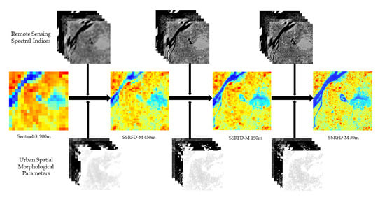
:Land surface temperature (LST) is one of the most important parameters in urban thermal environmental studies. Compared to natural surfaces, the surface of urban areas is more complex, and the spatial variability of LST is higher. Therefore, it is important to obtain a high-spatial-resolution LST for urban thermal environmental research. At present, downscaling studies are mostly performed from a low spatial resolution directly to another high resolution, which often results in lower accuracy with a larger scale span. First, a step-by-step random forest downscaling LST model (SSRFD) is proposed in this study. In our work, the 900-m resolution Sentinel-3 LST was sequentially downscaled to 450 m, 150 m and 30 m by SSRFD. Then, urban spatial morphological parameters were introduced into SSRFD, abbreviated as SSRFD-M, to compensate for the deficiency of remote-sensing indices as driving factors in urban downscaling LST. The results showed that the RMSE value of the SSRFD results was reduced from 2.6 °C to 1.66 °C compared to the direct random forest downscaling model (DRFD); the RMSE value of the SSRFD-M results in built-up areas, such as Gulou and Qinhuai District, was reduced by approximately 0.5 °C. We also found that the underestimation of LST caused by considering only remote-sensing indices in places such as flowerbeds and streets was improved in the SSRFD-M results.
1. Introduction
As an important physical variable driving the energy exchange between the surface and the atmosphere, the surface temperature (LST) is one of the key parameters for studying the energy balance of the surface at global or regional scales. Currently, LST is widely used to assess surface moisture and drought levels [1,2,3,4], calculate urban heat island intensity [5,6,7] and simulate surface energy exchange [8,9,10,11]. In urban areas, the spatial and temporal heterogeneity of urban surface temperature is obvious due to the extremely complex surface, the strong differences in three-dimensional spatial geometry and the variety of surface components and types. Therefore, studies of the urban thermal environment and other urban-related research fields usually require LST data with a higher spatiotemporal resolution.
The LST data obtained by thermal infrared remote-sensing technology generally have the problem of conflicting spatial and temporal resolutions. For example, the Moderate Resolution Imaging Spectroradiometer (MODIS) LST product has a high temporal resolution, but the spatial resolution is only 1000 m; Sentinel-3 operates through a binary orbit with a temporal resolution of fewer than 0.9 days, but the spatial resolution of the LST product is also 1000 m; the land surface temperature product retrieved from Landsat TIRS has a spatial resolution of 100 m, but the revisit period is as long as 16 days. Together with the influence of clouds, the available valid Landsat LST data are even further diminished. High-temporal-resolution data are difficult to generate for refined surface temperature studies at an urban scale due to their low spatial resolution, while the high spatial resolution LST data are unable to study the variation pattern of LST in time due to their low temporal resolution. To solve the contradiction of spatial and temporal resolutions of remote-sensing thermal data, scholars have proposed a large number of technical methods from various perspectives, such as image processing and statistical regression, to obtain land surface temperature data with high spatial and temporal resolutions.
The statistical regression method has gained wide application in LST downscaling studies due to its low computational complexity and satisfactory downscaling results. The application of this method has become relatively mature in suburban and mountainous areas with simple land covers at a large spatial scale [12,13]. However, there are two problems that cannot be ignored when applying the statistical method to urban areas with complex land surface types. Firstly, the larger the spatial resolution span of the downscaling, the lower the accuracy tends to be. From the available thermal infrared remote-sensing data, there are lots of LST products with a higher temporal resolution at about 1000-m spatial resolution. When they are downscaled to the 100-m level or even the 10-m level, the spatial resolution of the downscaled LST differs from the original resolution by a factor of 10 or even 100, and the downscaled accuracy decreases as the spatial resolution increases. The main reason for this problem is that the assumption of a “constant spatial scale relationship” between LST and the driving factor does not hold when the resolution difference is large. Secondly, the traditional two-dimensional remote-sensing spectral indices and surface parameters are not sufficient to accurately describe the spatial pattern of an urban surface. Currently, commonly used remote-sensing indices for downscaling models, such as the normalized difference vegetation index (NDVI), normalized difference moisture index (NDMI), normalized difference water index (NDWI) and normalized difference building index (NDBI) [14] use surface parameters including the DEM, slope, slope direction, latitude, longitude and surface cover type [15,16], as well as multispectral data [17] describing the vegetation cover, moisture status and topographic relief of the land surface from the two-dimensional perspective. In contrast, cities are dominated by buildings and impervious pavements, but the influence of the three-dimensional morphological structure on local land surface temperature is less considered. In fact, a large number of studies have demonstrated that urban spatial morphological parameters such as the sky view factor (SVF), frontal area index (FAI) and building density (BD) are closely related to LST [18,19,20,21], meaning they need to be considered in downscaling models.
To address the above two problems, this study aimed to develop a step-by-step LST downscaling method by further considering urban spatial morphological parameters to obtain the urban land surface temperature at a spatial resolution of 30 m with high accuracy. The paper takes the central urban area of Nanjing, Jiangsu Province, China as the study area, and selects multi-source remote-sensing data, three-dimensional spatial distribution data of urban buildings to downscale the Sentinel-3 LST with the spatial resolution of 1000 m to the resolutions of 450, 150 and 30 m step-by-step using surface 2D and 3D parameters as driving factors. The downscaling results are evaluated by Landsat TIRS LST at the resolution of 30 m. Then, the influence of urban spatial morphological parameters on land surface temperature downscaling is discussed. The step-by-step LST downscaling method changes the traditional studies that directly downscale LST from a low spatial resolution to a high one, selecting several spatial resolutions for the intermediate downscaling process. The intermediate downscaling process is equivalent to supplementing the model with the land surface information and reducing the difference in spatial resolution, thus ensuring that the statistical regression model varies less with the spatial scale.
2. Research Review
A lot of research has been carried out on land surface temperature downscaling by scholars around the world. The main methods used for LST downscaling can be divided into two categories: image-based spatiotemporal fusion and kernel-driven downscaling methods.
The image fusion method obtains a high spatial and temporal resolution land of surface temperature by constructing a model to generate fused images, based on the combined weight of spectral, temporal and spatial information, by selecting similar images in the spatiotemporal neighborhood to be fused. Unlike the statistical downscaling method, the image fusion method does not directly model the relationship between land surface temperature and influencing parameters at low-spatial-resolution scales. Classical algorithms are as follows. Weng et al. [22] improved the STARFM model to establish the relationship between MODIS and TM radiometric brightness by linear spectral mixing analysis, and proposed a spatiotemporal adaptive fusion algorithm (SADFAT) for land surface temperature downscaling. Wu et al. [23] proposed a spatiotemporal integrated temperature fusion model (STITFM) for estimating high-spatiotemporal-resolution LST from multi-scale polar and geostationary orbiting satellite observations. The image fusion-based approaches assume that the radiative brightness for similar pixels behaves consistently at any spatial resolution, while in practice, the radiative brightness will inevitably vary in space and time. So, this approach generally performs poorly in urban areas with high-spatial-heterogeneity characteristics.
Kernel-driven downscaling methods can be classified into physical models and statistical regression methods according to whether the model is physically meaningful or not. Physical downscaling methods establish the relationship between LST and auxiliary data by using the physical mechanism of a mixture pixel and the thermal radiation principle. In this way, low-spatial-resolution pixels are decomposed to multiple subpixels to obtain the high-spatial-resolution LST. For example, L.J and Moore [24] developed the pixel block intensity modulation (PBIM) method to improve the spatial information in the low-spatial-resolution thermal infrared band by using multispectral data with a high spatial resolution. Nichol [25] proposed the emissivity modulation (EM) model to improve the spatial resolution of thermal radiation by using land surface emissivity and land cover data. Wang et al. [26] downscaled MODIS LST to a 30-m resolution based on the thermal decomposition equation. However, the design of physical models is usually difficult and the models are computationally complex and time-consuming.
The basic principle of a statistical regression method is to assume that the relationship between land surface temperature and driving factors does not change with the spatial scale. A statistical regression model is built using the low-spatial-resolution LST and the drivers, after which the high-spatial-resolution drivers are added to the model to predict the high-spatial-resolution LSTs. Up to now, the statistical regression method is the most widely used method in LST spatial downscaling studies. Based on the number of driving factors, statistical regression methods can be divided into single- and multi-factor models. For example, Distrad models used NDVI as the driver [27], and the TsHARP model used vegetation cover instead of NDVI [28]. In addition, Anthony et al. [29] developed a high-resolution urban thermal fusion (HUTS) technique to downscale Landsat TIRS to 30 m based on NDVI and surface albedo. Lacerda et al. [30] used the TsHARP model to downscale the MODIS LST to a high spatial resolution of 10 m. Vaculik et al. [31] downscaled the GOES-R LST with the resolution of 2000 m to 30 m by establishing a linear relationship between NDVI and LST. J.M. et al. [32] modified the TsHARP algorithm to downscale MODIS LST data covering one Spanish farm. However, single-factor models are only applicable to a region with high vegetation cover; they do not perform well in urban or arid areas, limited by the predictor variables. Multi-factor models with multiple remote-sensing indices and land surface parameters as driving factors were gradually proposed and applied. For example, Liu et al. proposed the G_Distrad model by adding NDBI and NDWI to the traditional Distrad model [14]. Pereira et al. [33] proposed a geographically weighted regression model (GWRK) by using NDVI and multispectral data to downscale the ASTER thermal infrared data for the natural regions and urban areas of Pantanal, Brazil. Considering the complex nonlinear relationships between land surface temperature and various geophysical parameters in urban areas [12,13], the three-layer structural (TLC) model [34], neural network [35], support vector machines [6], random forests [36] and other multivariate nonlinear statistical models have been continuously developed and applied to urban LST downscaling studies. Random forest models have been widely used in urban LST downscaling studies in recent years because of their low model complexity, fast training speed and ability to effectively avoid overfitting problems. Li et al. [36] compared three machine learning algorithms, random forest (RF), support vector machine (SVM) and artificial neural network (ANN), to the traditional TsHARP method in both urban and suburban areas of Beijing, and found that the LST downscaling accuracy of the machine learning algorithm was higher than that of the TsHARP algorithm. Wang et al. [37] compared the downscaling results from a multiple linear regression model (MRL), TsHARP model and random forest (RF), and found that the RF model is more suitable for heterogeneous surfaces such as urban areas. Ebrahimy et al. [38] used an adaptive random forest regression method to downscale MODIS LST over Iran to 30 m in the GEE platform. Njuk et al. [39] proposed an improved downscaling method for low-resolution thermal data based on minimizing the spatial mean bias of random forest, and the results demonstrated that the method reduces the inherent mean bias in the LST downscaling process and is more suitable for LST downscaling applications in complex environments. Here, we comprehensively analyzed most land surface temperature downscaling methods and built global models and assumed that the statistical relationships were spatially invariant, however, global models may produce large errors in local area applications. In recent years, many scholars have devoted their work to using local models to capture the spatial non-stationary characteristics of land surface variables, and then established the local relationships between LST and influencing factors to improve the accuracy of LST downscaling [15].
3. Materials and Methods
3.1. Study Area
The central urban region of Nanjing, Jiangsu Province, China was chosen as the study area because it contains a variety of underlying surface types such as buildings, vegetation and water bodies, which helps to carry out land surface temperature downscaling studies of complex ground cover types. Figure 1 presents a true-color image and building distribution map of the study area at a spatial resolution of 10 m.
The study area includes several urban administrative districts, including the Qixia, Xuanwu, Gulou, Qinhuai and Jianye Districts, with an area of approximately 18 × 18 km2. The study area is located in the central region of the lower Yangtze River, with geographic coordinates between 31°14′N and 32°37′N and 118°22′E and 119°14″E. The total built-up area is approximately 823 km2. Although the study area is near a hilly area, the topography is flat, and there are many low hills and gentle hills. Nanjing has a humid subtropical climate with four distinct seasons, abundant rainfall and significant temperature differences between winter and summer. The average annual precipitation is 1106 mm, and the average annual temperature is 15.4 °C. Nanjing had a population of 10,312,200 at the end of 2019, with a resident population of 8.5 million, including 7.072 million in urban areas, and an urbanization rate of 83.2%. Nanjing is one of the economic-center cities in China, with a regional GDP of $1.6 billion in 2021.
3.2. Data
The Sentinel-3 LST product at a 1000-m spatial resolution for downscaling and Sentinel-2 multispectral image data were downloaded from the ESA website (https://scihub.copernicus.eu/dhus/#/home, accessed on 14 May 2022). The Landsat LST product at a 30-m spatial resolution for validation of downscaling results was downloaded from the USGS website (https://earthexplorer.usgs.gov/, accessed on 30 December 2021). Sentinel-2 visible light and shortwave infrared bands (B2–B4, B8, B11 and B12) were used to calculate normalized remote-sensing spectral indices. Nanjing downtown building and wind data were used to calculate urban spatial morphological parameters. Nanjing wind data from 2016 to 2020 were used to calculate the wind direction frequency, which were downloaded from the China Air Quality Online Monitoring and Analysis Platform (https://www.aqistudy.cn/historydata/, accessed on 14 May 2022). The details of all the data involved in this study are presented as follows.
3.2.1. Landsat LST Product
Landsat LST products were generated by EROS based on a single-channel inversion algorithm, by using the Landsat C2L1 thermal infrared band and other ancillary data [40,41]. Landsat LST products were resampled from 100 to 30 m for release to users by EROS using the nearest-neighbor resampling method. The Landsat LST images used in this study were imaged at 10:37 a.m. on 4 October 2021, with orbital row/column numbers 120/038 [42].
3.2.2. Sentinel-3 LST Product
The Sentinel series is an Earth observation satellite mission of the European Copernicus program. Sentinel-3 carries a variety of payloads, such as OLCI (sea and land colorimeter) and SLSTR (sea and land surface temperature radiometer), which are mainly used for high-precision measurements of the sea surface topography, sea and surface temperatures, ocean water color and soil properties [43]. Both 3A and 3B satellites in orbit have revisit periods of less than one day for areas within 30° latitude of the equator. SLSTR has six solar reflection bands (S1–S6) and four thermal infrared bands (S7–S9, F1, F2) with spatial resolutions of 500 and 1000 m, respectively. The Sentinel-3 LST products are produced by a split-window algorithm using three bands of S7–S9 and other auxiliary data, and the products are accurate to 1 K. The LST product of Sentinel-3B SLSTR was selected for this study, with an imaging time of 10:04 am on 4 October 2021. The Sentinel LST was resampled to a spatial resolution of 900 m by using the bilinear interpolation method for downscaling in this study to match the reference LST with a spatial resolution of 30 m.
3.2.3. Sentinel-2 Multispectral Data
Sentinel-2 is a multispectral high-resolution imaging satellite with two satellites in orbit, 2A and 2B, with a revisit period of five days [44]. Each satellite carries a multispectral imager (MSI), which can cover 13 spectral bands with ground resolutions of 10, 20 and 60 m and an amplitude of 290 km. The blue, green, red, and near-infrared bands needed for this study are the B2, B3, B4 and B8 bands of the Sentinel-2 satellite, each with a resolution of 10 m. B11 and B12 are shortwave infrared bands with a resolution of 20 m, resampled to 10 m to match the visible bands.
3.2.4. Urban Building Data
The building data used in this study were provided by Urban Data Corps, obtained in around 2012. Urban Data Corps is ranked in the top 10 in the big-data field according to the 2017 China Big Data Development Report published by the National Information Center of China. Urban Data Corps can provide a variety of high-precision data for urban research.
The building vector data contain the polygon of the building distribution, building floor data and building height data in a shapefile format with the WGS-84 coordinate system. Comparing the urban building distribution data with satellite images in 2012, we found that the building location and outline highly overlap with the satellite images, and the building floor number is also very consistent with the field survey results, which indicates the high accuracy of the building distribution data. The field survey found that the ground cover types in most of the study areas, such as Gulou District and Qinhuai District, did not change significantly between 2012 and 2021, except for Qixia District. In this study, the building vector data in the shapefile format were firstly converted to raster data in the TIF format with a spatial resolution of 10 m. After that, the urban spatial morphological parameters were calculated based on the building raster data and other auxiliary data using corresponding formulas.
3.3. Calculation of the Downscaling Driving Factor
3.3.1. Calculation of the Remote-Sensing Spectral Index
The L2A-level surface reflectance data from Sentinel-2B were selected for this study to calculate remotely sensed spectral indices that are closely related to surface temperature, including the modified normalized difference water index (MNDWI), normalized difference building index (NDBI), normalized difference built-up and soil index (NDBSI) [28], normalized difference moisture index (NDMI), normalized difference vegetation index (NDVI) and soil adjusted vegetation index (SAVI). The calculation process was performed using SNAP 8.0, a professional piece of software for data-processing in the Sentinel series. The calculation formula is shown in Table 1.
3.3.2. Calculation of Urban Spatial Morphological Parameters
The building vector data of Nanjing were converted to raster data with a 10-m resolution to calculate urban spatial morphological parameters including the building density (BD), frontal area density (FAD), floor area ratio (FAR), mean height (MH) and sky view factor (SVF). The SVF was calculated by the raster algorithm. The influence of buildings within a radius of 100 m was considered when calculating the SVF of each pixel. FAD was calculated using the building raster data and the wind direction frequency data by a self-developed raster algorithm with a plot area of 100 × 100 m2. Other spatial morphological parameters, such as BD, FAR and MH, were calculated using 10-m building raster data and the corresponding equations in Table 2 with a plot area of 100 × 100 m2.
3.4. Downscaling LST Method Based on Random Forest
The core idea of surface temperature downscaling is the invariance of the relationship between LST and driving factors at different spatial resolutions so that the statistical relationship between LST and the regression kernel at a low resolution can be applied to a high spatial resolution to complete the downscaling process. The specific formulas are as follows:
where varc denotes the low-resolution explanatory variable, varf denotes the high-resolution explanatory variable, Tc denotes the low-resolution LST, Tc’ denotes the predicted low-resolution LST, ΔT denotes the simulation residual and Tf’ denotes the predicted high-resolution LST.
This study used the random forest algorithm to construct the LST downscaling model. Random forest is an integrated decision tree-based learning algorithm proposed by Breiman in 2001 as a supervised learning algorithm [32]. The algorithm uses the bootstrap resampling method to randomly select samples from the training sample set. The extracted bootstrap samples are trained separately for each decision tree, and an algorithm for randomly selecting a subset of features is introduced in the process of splitting the nodes of the decision tree. The prediction results of each decision tree are counted and voted on to obtain the final prediction results of the input data. The random forest algorithm has stronger noise immunity than other algorithms because of the introduction of randomly selected training samples and randomly selected feature subsets that make the correlation among each decision tree smaller. The random forest algorithm is better at handling nonlinear problems than traditional statistical regression algorithms. As long as the number of decision trees is sufficient, the random forest algorithm can effectively avoid the overfitting problem, and the training speed is faster. The random forest algorithm can examine the interaction between features during the training process and output the feature importance, which is a reference for analyzing the degree of influence of features. In this study, the experimental dataset was divided into training and validation datasets according to the ratio of 8:2. The main parameters that need to be set manually to build a random forest downscaling model using the Pycharm platform include the number of decision trees (n_estimators) and the maximum number of features (max_features). n_estimators refers to the number of decision trees built in the random forest, which was set to 700 after testing in this study. max_feature refers to the maximum number of features selected when building each decision tree, which was set to log(n_estimators) in this study. Other parameters were set to default values.
3.5. Step-By-Step Random Forest Downscaling Method (SSRFD)
When the spatial resolution spans a larger range, the downscaling results cannot accurately characterize the spatial distribution of LST, which tends to underestimate the surface temperature in building areas and overestimate it for water bodies and vegetated areas. This study proposed a step-by-step downscaling LST method based on the random forest model (SSRFD), which achieves a significant increase in the spatial resolution of LST without excessive loss of accuracy through multiple, small-scale spatial resolution downscaling processes. During the SSRFD model’s work, each intermediate downscaling adds additional and finer surface information to the model. In this way, models are trained to accurately express the relationship between land surface temperature and driving factors.
In this study, the direct random forest downscaling (DRFD) method was performed to directly downscale 900-m Sentinel-3 LST to a 30-m resolution, and then two downscaling methods were conducted using the proposed SSRFD method. The first method, named SSRFD, downscaled the 900-m Sentinel-3 LST to 30 m after 450 m and 150 m sequentially, where the SSRFD was driven by the six remote-sensing indices mentioned above. The second method, named SSRFD-M, downscaled 900-m Sentinel-3 LST to 30 m by the same process through SSRFD, where five additional urban spatial morphological parameters were added as the SSRFD driver factors. After that, LST downscaling results of DRFD, SSRFD and SSRFD-M were compared at a 30-m spatial resolution, which were all evaluated by using the 30-m Landsat-8 LST as the reference. Moreover, the influence of urban spatial morphological parameters on LST was analyzed based on SSRFD-M at a 30-m spatial resolution.
3.6. Accuracy Evaluation Methods
Pearson’s correlation coefficient (r), the mean absolute error (MAE) and root mean square error (RMSE) were used to comprehensively evaluate the downscaling results. Meanwhile, the maximum/minimum, mean (Mean) and standard deviation (SD) were calculated to evaluate the spatial variability characteristics of LST images before and after downscaling. The SD can reflect the spatial variability of thermal features.
4. Results
4.1. Comparison of the Results Obtained with SSRFD and DRFD
To reduce data differences caused by different sensors and LST inversion algorithms and increase the comparability and verifiability between Landsat-8 and Sentinel-3 LST products, a simple linear correction was applied to Sentinel-3 LST before the downscaling work. After performing the linearity correction, the maximum, minimum and mean values of Sentinel-3 LST changed from 38.80, 27.57 and 35.18 °C to 41.25, 30.84 and 37.90 °C, respectively, which were closer to Landsat LST in the range of values. The RMSE of the two LST products changed from 3.22 to 1.59 °C, indicating that the systematic differences between Sentinel-3 LST and Landsat LST were reduced to some extent.
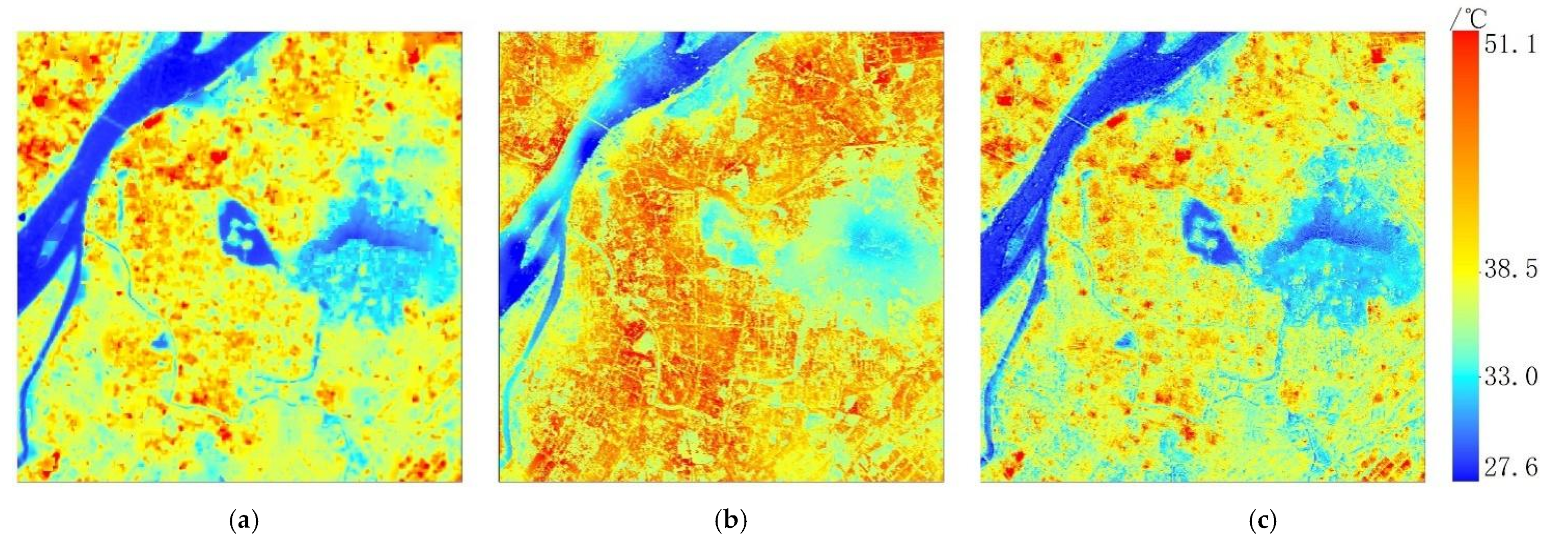
Comparative plots of the downscaling results are given in Figure 2, where the 900-m Sentinel-3 LST was downscaled to 30 m using the DRFD method and SSRFD method. Comparing Figure 2b,c with Figure 2a, both results captured finer spatial discrepancy characteristics and texture features, and the resulting LST distribution is basically consistent with Landsat LST. However, according to Figure 2b, there are large areas of high-temperature regions in the study area. The results obtained with DRFD as a whole are significantly overestimated. For example, the regions along the northwestern coast of the Yangtze River, Xuanwu Lake and Zijinshan Mountain show obvious temperature overestimation errors. The difference characteristics between the high-temperature region and the sub-high-temperature region are less clearly expressed than Landsat LST in Figure 2a. In contrast to Figure 2b, the results obtained with SSRFD (Figure 2c) captured the spatial distribution differences and textural characteristics more accurately. The distribution characteristics of both the building high-temperature zone and the water and vegetation low-temperature zone are in good agreement with Figure 2a. Overall, the results obtained with DRFD show an overall underestimation of the high-temperature region and an overestimation of the low-temperature region, which cannot accurately depict the spatial distribution pattern of LST in the study area.
The statistics (Table 3) show that the results from DRFD, with an SD of 2.64, are 0.82 lower than Landsat LST, but their mean value is 1.41 °C higher than Landsat LST. This is consistent with the performance of the DRFD results in Figure 2b, which further illustrates the overall high surface temperature predicted by DRFD. In comparison, the maximum, mean and SD of the results from SSRFD are 50.76, 36.78 and 3.73 °C, respectively, which only differ from the corresponding index of Landsat LST by approximately 0.3 °C. In summary, the downscaling results of SSRFD are more accurate, which is also demonstrated in Figure 3.
According to Figure 3, The histogram curves of SSRFD results fit better with that of the Landsat LST, as they both have clear “peak” values between 27.5–29 and 37–39 °C, which indicates that the SSRFD results are reasonable overall. The DRFD results differ significantly from the Landsat LST in terms of histogram shape characteristics, data distribution interval and data value range, e.g., the “peaks” of the results from DRFD are distributed between 40 and 41 °C. Overall, Figure 3 shows that the dense temperature interval of the image element distribution of DRFD is higher than that of SSRFD LST and Landsat LST.
Furthermore, the corresponding scatterplots of the two downscaling results from SSRFD and DRFD with Landsat LST are given in Figure 4a,b, respectively. According to Figure 4, the correlation r value between the DRFD results and Landsat LST is 0.6, while the SSRFD results improve this to 0.81. The MAE and RMSE values of the DRFD results are 2 and 2.6 °C, respectively, while the SSRFD results decrease to 1 and 1.66 °C, respectively. This indicates that using the SSRFD method can obtain a higher-accuracy LST than the DRFD method when the spatial resolution spans a large range.
4.2. Influence of Urban Spatial Morphological Parameters on Downscaling LST
4.2.1. Analysis of the Overall Downscaling Results in the Study Area
To evaluate the influence of urban spatial morphological parameters on LST downscaling, the five spatial morphological parameters calculated in Table 2 were introduced into the driving factors of SSRFD to downscale Sentinel-3 LST from a spatial resolution of 900 to 30 m. The downscaling results were also validated by Landsat LST.
Figure 5a,b shows the correlation plots of Landsat LST with the results from SSRFD and SSRFD-M, respectively, at a 30-m spatial resolution, where r improves from 0.81 to 0.85 and RMSE decreases from 1.66 to 1.44 °C after adding the spatial morphological parameters. The statistical histograms of Landsat LST and downscaling results are given in Figure 6. Compared to the SSRFD result, SSRFD-M is more matched with Landsat LST in distribution shape, especially between 35 and 40 °C where buildings and concrete pavements are mainly distributed. Otherwise, the features with temperatures between 28 and 35 °C are mainly vegetation and water bodies. The curves of the two downscaling results in this interval are higher than Landsat LST, indicating that there may be some LST overestimation in downscaling results for vegetation and water body areas. Combined with the analysis of Figure 5, we conclude that the SSRFD-M model performs better than SSRFD, especially for dense building areas.
4.2.2. Analysis of Regional Downscaling Results in the Study Area
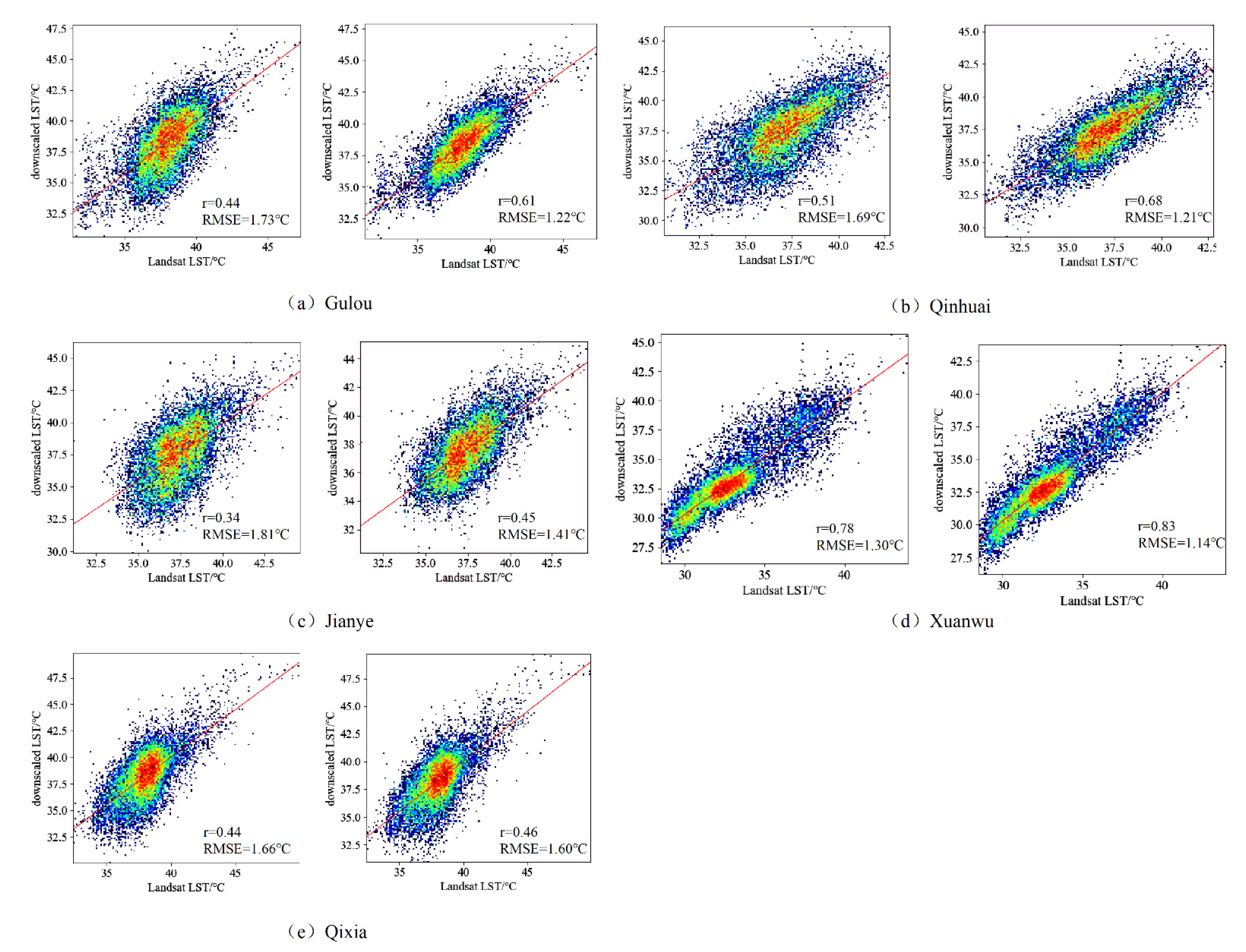
In Section 4.2.1, we found that the spatial morphological parameters have some favorable effects on the LST downscaling, especially for building areas. However, we remained unaware of how the urban spatial morphological parameters affect the LST downscaling results for different locations within the study. In this section, we intend to discuss the downscaling results for five subregions at a 30-m resolution to further analyze the role of urban spatial morphological parameters in the downscaling process. The distribution of correlations between the downscaling results and Landsat LST for five subdistricts, Qixia, Gulou, Xuanwu, Qinhuai and Jianye, are given in Figure 7. The influence of urban spatial morphological features on LST downscaling can be further verified because of the complexity of the urban ground cover types considered.
Figure 7a–c shows that the r value of the SSRFD-M downscaling results for the Gulou, Qinhuai and Jianye Districts improves from 0.44, 0.51 and 0.34 to 0.61, 0.68 and 0.45, respectively, while the RMSE value decreases from 1.73, 1.69 and 1.81 °C to 1.22, 1.21 and 1.41 °C, respectively. According to the statistical analysis of different areas, all three areas are located in a dense area of middle-rise buildings [33], where buildings and impervious surfaces dominate and the vegetation distribution is relatively low and sparse. Therefore, the LST distribution is closely related to the spatial morphological characteristics of buildings. These figures all exhibit that the downscaling results of SSRFD underestimated the LST for some regions between 35 and 40 °C. According to Figure 7d, r and RMSE values changed from 0.78 and 1.30 °C to 0.83 and 1.14 °C before and after considering spatial morphological parameters in Xuanwu District, respectively, with a slightly smaller improvement in accuracy relative to the Gulou and Qinhuai Districts. Statistically, among the Xuanwu District covered by the study area, non-built-up areas such as Zhong Shan Scenic Area and Xuanwu Lake account for approximately 50% of the district. Therefore, the inclusion of spatial morphological parameters has less influence on the downscaling results of these areas. If the downscaling results of building areas in Xuanwu District are counted separately, the RMSE of SSRFD-M decreases from 1.96 to 1.17 °C compared to the SSRFD results, which proves that SSRFD-M can effectively improve the downscaling effect in dense building areas. Figure 7e indicates that the SSRFD-M results for Qixia only improved/decreased r and RMSE values by 0.02/0.06 °C, respectively, compared to SSRFD. The reason for this is mainly the difference in years between Sentinel-3 LST data and building data. The type of land surface cover in some regions of Qixia has changed significantly. For example, the eastern side of Ningluo Expressway and the northern side of Qixia Avenue have changed from natural surfaces to building and road types. The building data used cannot accurately express the spatial morphological characteristics of these areas and cannot effectively improve the accuracy of LST downscaling. In addition, we found that a spatial resolution of 30 m may not be sufficient to show the surface temperature distribution pattern inside complex building areas.
We further selected five building-dense areas near the western side of Xuanwu Lake, Xinjiekou, Nanjing Museum, Nanjing Forestry University and the Olympic Sports Center, for downscaling results comparison, as shown by A, B, C, D and E in Figure 8a, respectively. A comparative analysis of the downscaling results with and without including spatial morphological parameters was carried out, and the results are shown in Figure 8b. When comparing the local downscaling results of SSRFD with SSRFD-M, it can be found that the regional LST of the vegetation-covered regions in the built-up area changed after considering the spatial morphological parameters. According to the SSRFD results of A1–E1, vegetation-covered areas near buildings, such as streets planted with trees and flowerbeds, showed a clear low-temperature zone (approximately 30–33 °C), which was 5–8 °C lower than the surface temperature of nearby building areas (approximately 35–40 °C). In contrast, the temperature in the corresponding regions illustrated by A2–E2 was only approximately 3–5 °C lower than that of the nearby buildings. No obvious low-temperature regions appeared in A2–E2, which were more consistent with the Landsat LST. Therefore, this study infers that the underestimation of LST generated by the SSRFD using only remote-sensing spectral indices was partially eliminated in SSRFD-M.
4.3. Parameter Importance Analysis of LST Downscaling
The importance of each driver at 90-, 450-, 150- and 30-m resolutions calculated by the random forest model is shown in Figure 9. According to Figure 9a, the NDBI has the highest importance at a 900-m resolution without spatial morphological parameters, which indicates that the NDBI is significantly correlated with LST in urban areas. With the increase in spatial resolution, the importance of the NDBI tends to decrease, and it drops to the lowest value (25%) at a 30-m resolution. Vegetation moisture is an important factor affecting LST in urban areas at any spatial resolution because the importance of the NDMI is maintained at 28–30% as the spatial resolution changes. The importance of the MNDWI increases from 11 to 15%, and the NDVI increases from 8% to 11%, which indicates that the contribution of water bodies and vegetation to LST increases as the resolution increases. The reason could be that some smaller lakes, green areas and narrow rivers are identified at a high spatial resolution. Figure 9b shows that the overall importance of the remote-sensing index did not change significantly in the SSRFD. Among the spatial morphological parameters, the importance of BD, FAD, FAR and MH decreased with increasing spatial resolution, while the SVF increased from approximately 3% to approximately 6%. The reason for this is that the regional spatial morphological parameters, such as BD, FAD and FAR, calculated by a single size (100 × 100 m), cannot represent finer architectural information. Therefore, the regional spatial morphological parameters are less relevant to LST as the resolution increases. As shown in Figure 9a,b, compared to other remote-sensing indices (all variations were in a range of 1–3%), there was a significant decrease in the importance of the NDBI at lower resolutions of 900 and 450 m, from 30 and 29% in Figure 9a to 22 and 23% in Figure 9b, respectively. The spatial morphological parameters at a low resolution to some extent compensated for the deficiency of the NDBI in the description of the spatial morphological features of buildings.
5. Discussion
With respect to the scale effect of the land surface temperature downscaling model, Pu et al. [46,47] concluded that the “constant scale relationship” between LST and driving factors does not hold under certain conditions. Comparing Figure 2a with Figure 2b for the main urban area of Nanjing, when the spatial resolution spans 30 times, the direct downscaling results cannot accurately represent the spatial distribution of land surface temperature, and the root mean square error of the traditional DRFD model is 2.6 °C (Figure 4a). This is similar to LST downscaling results in different regions such as that covered by Njuki et al. [39] in Kenya, Valdes et al. [13] in an arid Antarctic river valley, Zhu et al. [15] in Beijing and Ebrahimy et al. [38] in Iran. When the Sentinel-3 LST was downscaled to 450, 300, 150 and 30 m using the DRFD method, respectively, the research process revealed a phenomenon where r gradually decreases while RMSE increases as the spatial resolution span increases step-by-step, which is consistent with Zhu et al. (2020) [14] and Cao (2020) [48]. Using the step-by-step downscaling model (SSRFD), the root mean square error of the LST downscaling for the whole study area decreases to 1.66 °C, and the accuracy improves by about 1 °C (Figure 4b). Tang et al. [16] conducted a second downscaling procedure using the LST spatial features extracted from the initial downscaling results and obtained a higher accuracy of downscaling result, similar to the results of this study. The step-by-step downscaling method reduces the spatial resolution difference before and after downscaling by adding an intermediate LST downscaling process between low (e.g., 1 km) and high resolutions (e.g., 30 m), from which we can approximate that the statistical downscaling model does not change with smaller scales. The SSRFD can obtain a higher accuracy for LST downscaling and is more suitable for downscaling studies in urban areas with complex surface coverage and high-LST spatial heterogeneity. However, 900 m was used as the initial resolution in the study, and the step-by-step downscaling of resolution was performed subjectively by integer multiples of 2, 3 and 5. To obtain better LST downscaling results, further studies may be needed to determine the optimal spatial resolution change during stepwise downscaling.
In recent years, due to the continuous development of spatial data-acquisition technology, urban 3D spatial distribution data are becoming more and more refined and can be better used to calculate various urban spatial morphological parameters at different scales. There are more and more studies selecting urban morphological parameters to analyze the urban thermal environment. For example, Middel et al. [19] validated the effects of urban morphology and landscape type on local microclimate zones in the semi-arid region of Phoenix, Arizona; Qaid et al. [20] further explored the effect of SVF on the thermal environment of streets with different orientations; Wong et al., Li et al. and Nichol et al. studied the characteristics of urban spatial morphology in Kowloon Peninsula, Hong Kong and confirmed that the urban spatial morphology profoundly affects the urban microclimate [49]. Based on the results of these studies, it appears that the spatiotemporal variability of the urban thermal environment is closely related to the spatial morphological parameters, and the influential role of these three-dimensional parameters needs to be considered in-depth in urban LST downscaling studies. In this study, based on the traditional two-dimensional surface parameters of the downscaling model, five spatial morphological parameters, SVF, FAD, FAR, BD and MH, were added to downscale the Sentinel-3 LST to a high spatial resolution of 30 m. It was found that the urban spatial morphological parameters did affect the spatial distribution of LST, especially for the built-up areas.
The downscaling errors in the five building-dense areas decreased by 0.51, 0.48, 0.4, 0.16 and 0.06 °C (Figure 7). Analysis of the importance of the driving factors showed that the importance of the urban spatial morphological parameters was lower than that of the 2D remote-sensing spectral index (Figure 9). The reason may be that the factors for BD, FAD, FAR and MH were calculated through a moving window of 100 × 100 m, making it difficult to accurately describe the 3D spatial features at a high spatial resolution of 30 m. Compared to the other four spatial morphological parameters, SVF can be calculated pixel by pixel, and its importance gradually becomes larger as the spatial resolution increases, which generally indicates that the role of urban spatial morphological parameters cannot be neglected for LST downscaling at higher spatial resolutions than 30 m. Li et al. [17] and Liu et al. [50] also mentioned the necessity of considering urban spatial morphological parameters in urban LST downscaling.
In terms of downscaling accuracy validation, due to the lack of real land surface temperature with a higher spatial resolution, we just downscaled LST to the resolution of 30 m. If there are LSTs at a high spatial resolution, such as the data collected by thermal infrared sensors loaded on unmanned aerial vehicles or field measurement temperature probes, LST downscaling for a higher spatial resolution could be performed to further discuss the influence of morphological parameters.
Finally, a global random forest downscaling model was established in the study. Considering the characteristics of different urban regions and establishing sub-regional local models to improve LST downscaling accuracy need to be further discussed. For example, Stewart et al. [51] proposed to establish local urban climate zones by considering building and land cover types, an approach that can be used to downscale LST for various climate zones. More accurate downscaling results may be obtained by further analysis of the relationship between LST and urban spatial morphological parameters based on local urban climate zones.
6. Conclusions
This study carried out downscaling LST in urban areas using the SSRFD and DRFD methods, and the downscaling effects of the two methods were compared and analyzed. Urban spatial morphological parameters were introduced in the driver to verify their role in high-spatial-resolution downscaling LST. From the above investigations, the following conclusions were drawn:
- (1)
- The 900-m LST was downscaled step-by-step on the order of 450, 150 and 30 m. Compared to the results obtained with DRFD, the r value between the SSRFD results and Landsat LST was improved by 0.21, and the RMSE value was reduced by 0.94 °C. The SSRFD results more accurately captured the spatial distribution characteristics of the surface temperature, including the high-temperature zone of buildings and the low-temperature zone of water and vegetation. The underestimation/overestimation phenomenon of DRFD resulting in large errors in the high/low temperature zone was avoided or attenuated when using the SSRFD method.
- (2)
- The results obtained with SSRFD-M were partially significantly improved in the Gulou, Qinhuai and Jianye built-up areas compared to SSRFD, in which r and RMSE values improved/decreased by approximately 0.15 and 0.46 °C, respectively. The phenomenon of low-temperature zones in vegetation-covered areas when only remote-sensing spectral indices were used was improved. The SSRFD-M results to some extent compensated for the deficiency of remote-sensing spectral indices used for urban LST downscaling.
In this study, 900 m was used as the initial resolution, and downscaling was carried out in integer multiples of 2, 3 and 5. Further research is needed to determine the optimal downscaling resolution change multiples to obtain better downscaling results. In addition, this paper established a random forest downscaling LST model for the study area as a whole, while urban climate zones could be divided according to building and land cover types. More accurate downscaling results may be obtained by further analysis of the relationship between LST and urban spatial morphological parameters based on urban local climate zones.
Author Contributions
Conceptualization, G.Z. and X.L.; methodology, G.Z. and S.Z.; software, X.L.; validation, Y.X.; data curation, X.L.; writing—original draft preparation, X.L.; writing—review and editing, G.Z. and Y.X.; project administration, G.Z.; funding acquisition, S.Z. and Y.X. All authors have read and agreed to the published version of the manuscript.
Funding
This research was supported by the National Natural Science Foundation of China (42171101, 41871028).
Data Availability Statement
Not applicable.
Acknowledgments
The authors would like to acknowledge the United States Geological Survey for the provision of the Landsat-8 LST product, and the European Space Agency for the provision of the Sentinel-3 LST product and Sentinel-2 remote-sensing data.
Conflicts of Interest
The authors declare no conflict of interest.
References
- Jaafar, H.; Mourad, R.; Schull, M. A Global 30-m ET Model (HSEB) Using Harmonized Landsat and Sentinel-2, MODIS and VIIRS: Comparison to ECOSTRESS ET and LST. Remote Sens. Environ. 2022, 274, 112995. [Google Scholar] [CrossRef]
- Paolini, G.; Escorihuela, M.J.; Bellvert, J.; Merlin, O. Disaggregation of SMAP Soil Moisture at 20 m Resolution: Validation and Sub-Field Scale Analysis. Remote Sens. 2022, 14, 167. [Google Scholar] [CrossRef]
- Joshi, R.C.; Ryu, D.; Sheridan, G.J.; Lane, P.N.J. Modeling Vegetation Water Stress over the Forest from Space: Temperature Vegetation Water Stress Index (TVWSI). Remote Sens. 2021, 13, 4635. [Google Scholar] [CrossRef]
- Chu, H.-J.; Wijayanti, R.F.; Jaelani, L.M.; Tsai, H.-P. Time Varying Spatial Downscaling of Satellite-Based Drought Index. Remote Sens. 2021, 13, 3693. [Google Scholar] [CrossRef]
- Baqa, M.F.; Lu, L.; Chen, F.; Nawaz-ul-Huda, S.; Pan, L.; Tariq, A.; Qureshi, S.; Li, B.; Li, Q. Characterizing Spatiotemporal Variations in the Urban Thermal Environment Related to Land Cover Changes in Karachi, Pakistan, from 2000 to 2020. Remote Sens. 2022, 14, 2164. [Google Scholar] [CrossRef]
- Sismanidis, P.; Bechtel, B.; Perry, M.; Ghent, D. The Seasonality of Surface Urban Heat Islands across Climates. Remote Sens. 2022, 14, 2318. [Google Scholar] [CrossRef]
- Niu, L.; Zhang, Z.; Peng, Z.; Jiang, Y.; Liu, M.; Zhou, X.; Tang, R. Research on China’s surface urban heat island drivers and its spatial heterogeneity. China Environ. Sci. 2021, 13, 4428. [Google Scholar]
- Romaguera, M.; Vaughan, R.G.; Ettema, J.; Izquierdo-Verdiguier, E.; Hecker, C.A.; van der Meer, F.D. Detecting Geothermal Anomalies and Evaluating LST Geothermal Component by Combining Thermal Remote Sensing Time Series and Land Surface Model Data. Remote Sens. Environ. 2018, 204, 534–552. [Google Scholar] [CrossRef]
- Hrisko, J.; Ramamurthy, P.; Yu, Y.; Yu, P.; Melecio-Vázquez, D. Urban Air Temperature Model Using GOES-16 LST and a Diurnal Regressive Neural Network Algorithm. Remote Sens. Environ. 2020, 237, 111495. [Google Scholar] [CrossRef]
- Westermann, S.; Langer, M.; Boike, J. Spatial and Temporal Variations of Summer Surface Temperatures of High-Arctic Tundra on Svalbard—Implications for MODIS LST Based Permafrost Monitoring. Remote Sens. Environ. 2011, 115, 908–922. [Google Scholar] [CrossRef]
- Mahour, M.; Tolpekin, V.; Stein, A.; Sharifi, A. A Comparison of Two Downscaling Procedures to Increase the Spatial Resolution of Mapping Actual Evapotranspiration. ISPRS J. Photogramm. Remote Sens. 2017, 126, 56–67. [Google Scholar] [CrossRef]
- Bartkowiak, P.; Castelli, M.; Notarnicola, C. Downscaling Land Surface Temperature from MODIS Dataset with Random Forest Approach over Alpine Vegetated Areas. Remote Sens. 2019, 11, 1319. [Google Scholar] [CrossRef] [Green Version]
- Lezama Valdes, L.-M.; Katurji, M.; Meyer, H. A Machine Learning Based Downscaling Approach to Produce High Spatio-Temporal Resolution Land Surface Temperature of the Antarctic Dry Valleys from MODIS Data. Remote Sens. 2021, 13, 4673. [Google Scholar] [CrossRef]
- Zhu, J.; Zhu, S.; Yu, F.; Zhang, G.; Xu, Y. A downscaling method for ERA5 reanalysis land surface temperature over urban and mountain areas. Natl. Remote Sens. Bull. 2021, 25, 1778–1791. [Google Scholar]
- Zhu, X.; Song, X.; Leng, P.; Hu, R. Spatial downscaling of land surface temperature with the multi-scale geographically weighted regression. Natl. Remote Sens. Bull. 2021, 25, 1749–1766. [Google Scholar]
- Tang, K.; Zhu, H.; Ni, P. Spatial Downscaling of Land Surface Temperature over Heterogeneous Regions Using Random Forest Regression Considering Spatial Features. Remote Sens. 2021, 13, 3645. [Google Scholar] [CrossRef]
- Li, N.; Wu, H.; Luan, Q. Land Surface Temperature Downscaling in Urban Area: A Case Study of Beijing. Natl. Remote Sens. Bull. 2021, 25, 1808–1820. [Google Scholar]
- Golany, G.S. Urban Design Morphology and Thermal Performance. Atmos. Environ. 1996, 30, 455–465. [Google Scholar] [CrossRef]
- Middel, A.; Häb, K.; Brazel, A.J.; Martin, C.A.; Guhathakurta, S. Impact of Urban Form and Design on Mid-Afternoon Microclimate in Phoenix Local Climate Zones. Landsc. Urban Plan. 2014, 122, 16–28. [Google Scholar] [CrossRef]
- Qaid, A.; Lamit, H.B.; Ossen, D.R.; Rasidi, M.H. Effect of the Position of the Visible Sky in Determining the Sky View Factor on Micrometeorological and Human Thermal Comfort Conditions in Urban Street Canyons. Theor. Appl. Climatol. 2018, 131, 1083–1100. [Google Scholar] [CrossRef]
- Xiong, Y.; Peng, F.; Zou, B. Spatiotemporal Influences of Land Use/Cover Changes on the Heat Island Effect in Rapid Urbanization Area. Front. Earth Sci. 2019, 13, 614–627. [Google Scholar] [CrossRef]
- Weng, Q.; Fu, P.; Gao, F. Generating Daily Land Surface Temperature at Landsat Resolution by Fusing Landsat and MODIS Data. Remote Sens. Environ. 2014, 145, 55–67. [Google Scholar] [CrossRef]
- Wu, P.; Shen, H.; Zhang, L.; Göttsche, F.-M. Integrated Fusion of Multi-Scale Polar-Orbiting and Geostationary Satellite Observations for the Mapping of High Spatial and Temporal Resolution Land Surface Temperature. Remote Sens. Environ. 2015, 156, 169–181. [Google Scholar] [CrossRef]
- Guo, L.J.; Moore, J.M. Pixel Block Intensity Modulation: Adding Spatial Detail to TM Band 6 Thermal Imagery. International J. Remote Sens. 1998, 19, 2477–2491. [Google Scholar] [CrossRef]
- Nichol, J. An Emissivity Modulation Method for Spatial Enhancement of Thermal Satellite Images in Urban Heat Island Analysis. Photogramm. Eng. Remote Sens. 2009, 75, 547–556. [Google Scholar] [CrossRef] [Green Version]
- Wang, J.; Schmitz, O.; Lu, M.; Karssenberg, D. Thermal Unmixing Based Downscaling for Fine Resolution Diurnal Land Surface Temperature Analysis. ISPRS J. Photogramm. Remote Sens. 2020, 161, 76–89. [Google Scholar] [CrossRef]
- Kustas, W.P.; Norman, J.M.; Anderson, M.C.; French, A.N. Estimating Subpixel Surface Temperatures and Energy Fluxes from the Vegetation Index-Radiometric Temperature Relationship. Remote Sens. Environ. 2003, 85, 429–440. [Google Scholar] [CrossRef]
- Agam, N.; Kustas, W.P.; Anderson, M.C.; Li, F.; Neale, C.M.U. A Vegetation Index Based Technique for Spatial Sharpening of Thermal Imagery. Remote Sens. Environ. 2007, 107, 545–558. [Google Scholar] [CrossRef]
- Dominguez, A.; Kleissl, J.; Luvall, J.C.; Rickman, D.L. High-Resolution Urban Thermal Sharpener (HUTS). Remote Sens. Environ. 2011, 115, 1772–1780. [Google Scholar] [CrossRef] [Green Version]
- Lacerda, L.N.; Cohen, Y.; Snider, J.; Huryna, H.; Liakos, V.; Vellidis, G. Field Scale Assessment of the TsHARP Technique for Thermal Sharpening of MODIS Satellite Images Using VENµS and Sentinel-2-Derived NDVI. Remote Sens. 2021, 13, 1155. [Google Scholar] [CrossRef]
- Vaculik, A.F.; Rachid Bah, A.; Norouzi, H.; Beale, C.; Valentine, M.; Ginchereau, J.; Blake, R. Downscaling of Satellite Land Surface Temperature Data Over Urban Environments. In Proceedings of the IEEE International Geoscience and Remote Sensing Symposium, Yokohama, Japan, 28 July–2 August 2019; pp. 7475–7477. [Google Scholar]
- Sánchez, J.M.; Galve, J.M.; González-Piqueras, J.; López-Urrea, R.; Niclòs, R.; Calera, A. Monitoring 10-m LST from the Combination MODIS/Sentinel-2, Validation in a High Contrast Semi-Arid Agroecosystem. Remote Sens. 2020, 12, 1453. [Google Scholar] [CrossRef]
- Pereira, O.J.R.; Melfi, A.J.; Montes, C.R.; Lucas, Y. Downscaling of ASTER Thermal Images Based on Geographically Weighted Regression Kriging. Remote Sens. 2018, 10, 633. [Google Scholar] [CrossRef] [Green Version]
- Guo, F.; Hu, D.; Schlink, U. A New Nonlinear Method for Downscaling Land Surface Temperature by Integrating Guided and Gaussian Filtering. Remote Sens. Environ. 2022, 271, 112915. [Google Scholar] [CrossRef]
- Guijun, Y.; Ruiliang, P.; Wenjiang, H.; Jihua, W.; Chunjiang, Z. A Novel Method to Estimate Subpixel Temperature by Fusing Solar-Reflective and Thermal-Infrared Remote-Sensing Data with an Artificial Neural Network. IEEE Trans. Geosci. Remote Sens. 2010, 48, 2170–2178. [Google Scholar] [CrossRef]
- Li, W.; Ni, L.; Li, Z.-L.; Duan, S.-B.; Wu, H. Evaluation of Machine Learning Algorithms in Spatial Downscaling of MODIS Land Surface Temperature. IEEE J. Sel. Top. Appl. Earth Obs. Remote Sens. 2019, 12, 2299–2307. [Google Scholar] [CrossRef]
- Wang, R.; Gao, W.; Peng, W. Downscale MODIS Land Surface Temperature Based on Three Different Models to Analyze Surface Urban Heat Island: A Case Study of Hangzhou. Remote Sens. 2020, 12, 2134. [Google Scholar] [CrossRef]
- Ebrahimy, H.; Aghighi, H.; Azadbakht, M.; Amani, M.; Mahdavi, S.; Matkan, A.A. Downscaling MODIS Land Surface Temperature Product Using an Adaptive Random Forest Regression Method and Google Earth Engine for a 19-Years Spatiotemporal Trend Analysis Over Iran. IEEE J. Sel. Top. Appl. Earth Obs. Remote Sens. 2021, 14, 2103–2112. [Google Scholar] [CrossRef]
- Njuki, S.M.; Mannaerts, C.M.; Su, Z. An Improved Approach for Downscaling Coarse-Resolution Thermal Data by Minimizing the Spatial Averaging Biases in Random Forest. Remote Sens. 2020, 12, 3507. [Google Scholar] [CrossRef]
- Malakar, N.K.; Hulley, G.C.; Hook, S.J.; Laraby, K.; Cook, M.; Schott, J.R. An Operational Land Surface Temperature Product for Landsat Thermal Data: Methodology and Validation. IEEE Trans. Geosci. Remote Sens. 2018, 56, 5717–5735. [Google Scholar] [CrossRef]
- Cook, M.; Schott, J.R.; Mandel, J.; Raqueno, N. Development of an Operational Calibration Methodology for the Landsat Thermal Data Archive and Initial Testing of the Atmospheric Compensation Component of a Land Surface Temperature (LST) Product from the Archive. Remote Sens. 2014, 6, 11244–11266. [Google Scholar] [CrossRef] [Green Version]
- LSDS-1619_Landsat-8-9-C2-L2-ScienceProductGuide-v4.pdf. Available online: https://d9-wret.s3.us-west-2.amazonaws.com/assets/palladium/production/s3fspublic/media/files/LSDS-1619_Landsat-8-9-C2-L2-ScienceProductGuide-v4.pdf (accessed on 30 December 2021).
- SLSTR_Level-2_LST_ATBD.pdf. Available online: https://sentinel.esa.int/documents/247904/0/SLSTR_Level-2_LST_ATBD.pdf/8a4322ef-c7e0-4abc-9cac-8f5fd69e1fd7 (accessed on 14 May 2022).
- S2-PDGS-TAS-DI-PSD-V14.9.pdf. Available online: https://sentinel.esa.int/documents/247904/4756619/S2-PDGS-TAS-DI-PSD-V14.9.pdf/3d3b6c9c-4334-dcc4-3aa7-f7c0deffbaf7 (accessed on 14 May 2022).
- Xu, H. A remote sensing urban ecological index and its application. Acta Ecol. Sin. 2013, 33, 7853–7862. [Google Scholar]
- Pu, R. Assessing Scaling Effect in Downscaling Land Surface Temperature in a Heterogenous Urban Environment. Int. J. Appl. Earth Obs. Geoinf. 2021, 96, 102256. [Google Scholar] [CrossRef]
- Pu, R.; Bonafoni, S. Reducing Scaling Effect on Downscaled Land Surface Temperature Maps in Heterogenous Urban Environments. Remote Sens. 2021, 13, 5044. [Google Scholar] [CrossRef]
- Cao, C.; Yang, Y. Downscaling Multi-resolution Land surface Temperature Research. Mod. Surv. Mapp. 2018, 41, 3–8. [Google Scholar]
- Wong, M.S.; Nichol, J.; Ng, E. A Study of the “Wall Effect” Caused by Proliferation of High-Rise Buildings Using GIS Techniques. Landsc. Urban Plan. 2011, 102, 245–253. [Google Scholar] [CrossRef]
- Liu, Y.; Xu, Y.; Zhang, F.; Shu, W. Influence of Beijing Spatial Morphology on the Distribution of Urban Heat Island. Acta Geogr. Sin. 2021, 76, 1662–1679. [Google Scholar]
- Stewart, I.D.; Oke, T.R. Local Climate Zones for Urban Temperature Studies. Bull. Am. Meteorol. Soc. 2012, 93, 1879–1900. [Google Scholar] [CrossRef]
Figure 1.
Sentinel-2 true-color composite image and building data of the study area (blue line represents the main urban area of Nanjing; red lines represent the study area boundaries).
Figure 1.
Sentinel-2 true-color composite image and building data of the study area (blue line represents the main urban area of Nanjing; red lines represent the study area boundaries).

Figure 2.
Spatial distribution of LST at 30-m spatial resolution. (a) Landsat reference LST. (b) Downscaled LST results of DRFD. (c) Downscaled LST results of SSRFD.
Figure 2.
Spatial distribution of LST at 30-m spatial resolution. (a) Landsat reference LST. (b) Downscaled LST results of DRFD. (c) Downscaled LST results of SSRFD.

Figure 3.
Histogram of downscaled LST and Landsat LST at 30-m resolution (black cubes refer to Landsat LST, red circles refer to downscaled LST obtained by the SSRFD method, blue triangles refer to downscaled LST obtained by the DRFD method).
Figure 3.
Histogram of downscaled LST and Landsat LST at 30-m resolution (black cubes refer to Landsat LST, red circles refer to downscaled LST obtained by the SSRFD method, blue triangles refer to downscaled LST obtained by the DRFD method).

Figure 4.
Scatterplots of the correlation analysis between downscaled LST and Landsat reference LST at a 30-m resolution. (a) Downscaled LST of Sentinel-3 from DRFD method. (b) Downscaled LST of Sentinel-3 from SSRFD method.
Figure 4.
Scatterplots of the correlation analysis between downscaled LST and Landsat reference LST at a 30-m resolution. (a) Downscaled LST of Sentinel-3 from DRFD method. (b) Downscaled LST of Sentinel-3 from SSRFD method.

Figure 5.
Scatterplots of the correlation analysis between downscaled LST and Landsat LST on the overall region at a 30-m resolution. (a) SSRFD result. (b) SSRFD-M result.
Figure 5.
Scatterplots of the correlation analysis between downscaled LST and Landsat LST on the overall region at a 30-m resolution. (a) SSRFD result. (b) SSRFD-M result.

Figure 6.
Histogram of downscaled LST and Landsat LST at a 30-m resolution (black cubes refer to Landsat LST, red circles refer to the SSRFD results and blue triangles refer to the SSRFD-M results).
Figure 6.
Histogram of downscaled LST and Landsat LST at a 30-m resolution (black cubes refer to Landsat LST, red circles refer to the SSRFD results and blue triangles refer to the SSRFD-M results).

Figure 7.
Scatterplot of correlation analysis between downscaled LST and Landsat LST at a spatial resolution of 30 m (downscaled LSTs obtained from SSRFD and SSRFD-M correspond to the left and right panels in a–e).
Figure 7.
Scatterplot of correlation analysis between downscaled LST and Landsat LST at a spatial resolution of 30 m (downscaled LSTs obtained from SSRFD and SSRFD-M correspond to the left and right panels in a–e).

Figure 8.
Spatial distribution of the downscaled LST at the resolution of 30 m in five localities of the study area (in b, A1–E1 refer to the downscaled LST from SSRFD, and A2–E2 refer to the downscaled LST from SSRFD-M). (a) Landsat LST. (b) the downscaled LST for representative 5 local area.
Figure 8.
Spatial distribution of the downscaled LST at the resolution of 30 m in five localities of the study area (in b, A1–E1 refer to the downscaled LST from SSRFD, and A2–E2 refer to the downscaled LST from SSRFD-M). (a) Landsat LST. (b) the downscaled LST for representative 5 local area.

Figure 9.
Importance of each driver at spatial resolutions of 900, 450, 150 and 30 m. (a) No spatial morphological parameters added. (b) Spatial morphological parameters added.
Figure 9.
Importance of each driver at spatial resolutions of 900, 450, 150 and 30 m. (a) No spatial morphological parameters added. (b) Spatial morphological parameters added.


Table 1.
Remote-sensing spectral indices required for downscaling and calculation formulas.
| Var. | Description | Equations |
|---|---|---|
| MNDWI | Improve the normalized difference water body index to highlight water body information | |
| NDBI | Normalize the difference building index to highlight building information | |
| NDBSI | Indicate the degree of dryness of the ground surface [45] | |
| NDMI | Indicate the vegetation moisture | |
| NDVI | Highlight vegetation information | |
| SAVI | Reduce the sensitivity of vegetation indices to changes in reflectance of different soils | L = 0.5 |
Notes: ρ1–ρ12 denote the surface reflectance of Sentinel-2 bands 1–12.
Table 2.
Urban spatial morphological parameters required for LST downscaling.
| Var. | Description | Equations |
|---|---|---|
| BD | Building Density | Ai indicates the ith building area and AT indicates the calculated plot area |
| FAD | Frontal Area Density | indicates the frequency of the wind direction θ, i = 1,…, 16 |
| FAR | Floor Area Ratio | the ith building area |
| MH | Mean Height | indicates the ith building height and n indicates the number of buildings |
| SVF | Sky View Factor | ψsky indicates SVF, β indicates the building height angle, H indicates the building height, X indicates the calculated radius and is set to 100 m in this study |
Note: Except for SVF, the plot area AT calculated by all other parameters takes the value of 100 × 100 m.
Table 3.
Statistical values of LST downscaled from DRFD, SSRFD methods and Landsat reference LST data at a 30-m resolution.
Table 3.
Statistical values of LST downscaled from DRFD, SSRFD methods and Landsat reference LST data at a 30-m resolution.
| Statistical Variables | Reference LST/°C | DRFD LST/°C | SSRFD LST/°C |
|---|---|---|---|
| Maximum | 51.06 | 42.80 | 50.76 |
| Minimum | 13.94 | 28.95 | 24.36 |
| Mean | 36.50 | 37.91 | 36.78 |
| Standard deviation | 3.46 | 2.64 | 3.73 |
Publisher’s Note: MDPI stays neutral with regard to jurisdictional claims in published maps and institutional affiliations. |
© 2022 by the authors. Licensee MDPI, Basel, Switzerland. This article is an open access article distributed under the terms and conditions of the Creative Commons Attribution (CC BY) license (https://creativecommons.org/licenses/by/4.0/).
Share and Cite
MDPI and ACS Style
Li, X.; Zhang, G.; Zhu, S.; Xu, Y. Step-By-Step Downscaling of Land Surface Temperature Considering Urban Spatial Morphological Parameters. Remote Sens. 2022, 14, 3038. https://doi.org/10.3390/rs14133038
AMA Style
Li X, Zhang G, Zhu S, Xu Y. Step-By-Step Downscaling of Land Surface Temperature Considering Urban Spatial Morphological Parameters. Remote Sensing. 2022; 14(13):3038. https://doi.org/10.3390/rs14133038
Chicago/Turabian StyleLi, Xiangyu, Guixin Zhang, Shanyou Zhu, and Yongming Xu. 2022. "Step-By-Step Downscaling of Land Surface Temperature Considering Urban Spatial Morphological Parameters" Remote Sensing 14, no. 13: 3038. https://doi.org/10.3390/rs14133038
Note that from the first issue of 2016, this journal uses article numbers instead of page numbers. See further details here.