Above-Ground Biomass Estimation for Coniferous Forests in Northern China Using Regression Kriging and Landsat 9 Images

Abstract

Accurate estimation of forest above-ground biomass (AGB) is critical for assessing forest quality and carbon stocks, which can improve understanding of the vegetation growth processes and the global carbon cycle. Landsat 9, the latest launched Landsat satellite, is the successor and continuation of Landsat 8, providing a highly promising data resource for land cover change, forest surveys, and terrestrial ecosystem monitoring. Regression kriging was developed in the study to improve the AGB estimation and mapping using the Landsat 9 image in Wangyedian forest farm, northern China. Multiple linear regression (MLR), support vector machine (SVM), back propagation neural network (BPNN), and random forest (RF) were used as the original models to predict the AGB trends, and the optimal model was used to overlay the results of kriging interpolation based on the residuals to obtain the new AGB predictions. In addition, Landsat 8 images in Wangyedian were used for comparison and verification with Landsat 9. The results showed that all bands of Landsat 8 and Landsat 9 maintained a high degree of uniformity, with positive correlation coefficients ranging from 0.77 to 0.89 (p < 0.01). RF achieved the highest estimation accuracy among all the original models based on the two data sources. However, kriging regression can significantly reduce the estimation error, with the root mean square error (RMSE) decreasing by 55.4% and 51.1%, for Landsat 8 and Landsat 9, respectively, compared to the original RF. Further, the R² and the lowest RMSE for Landsat 8 were 0.88 and 16.83 t/ha, while, for Landsat 9, they were 0.87 and 17.91 t/ha. The use of regression kriging combined with Landsat 9 imagery has great potential for achieving efficient and highly accurate forest AGB estimates, providing a new reference for long-term monitoring of forest resource dynamics.

1. Introduction

Forest above-ground biomass (AGB) provides a direct measure of forest quantity and quality, which is critical for forest health assessment [1,2]. Accurate AGB estimation can improve the understanding of the global carbon cycle and terrestrial ecosystem service functions [3,4]. In addition, periodic AGB monitoring can provide scientific information and guidance on forest quality, forest health status, and degradation to inform efficient forest resource management [5,6].

Compared to labor-intensive and time-consuming manual surveys, remote sensing technology is non-destructive and more efficient in forest surveys [7]. Periodic estimation of forest parameters using remote sensing data has become one of the main tools for regional forest resource survey and monitoring [8]. Optical images, synthetic aperture radar (SAR), and light detection and ranging (LiDAR) data are the main data sources for remote sensing estimation of forest parameters, which are also widely used for meteorological observation, natural resource monitoring, and geological survey [9,10,11]. As representatives of active remote sensing, SAR and LiDAR do not depend on solar radiation and can penetrate part of the forest canopy to obtain accurate information on the vertical structure of the forest [12,13,14]. SAR allows for all-weather and all-day exploration of Earth’s surface independent of weather and cloud cover. However, changes in terrain have a significant impact on the signal, which limits further application of SAR in forests with complex terrain [15]. LiDAR enables high-precision ranging of objects by emitting laser light, which can effectively characterize the ground information under the forest. As one of the representatives of LiDAR, terrestrial laser scanning (TLS) can obtain an accurate and detailed three-dimensional structure of the forest by scanning the forest from the bottom up [16]. However, the effects of weather and atmosphere and the arithmetic power consumption and processing efficiency of massive data are the main factors limiting it, and the effect of scrub shading on scanning and the limitation of scanning range and efficiency of TLS make it difficult to obtain LiDAR coverage over a large area [17]. In addition, high-density aerial LiDAR and satellite-based LiDAR can obtain vertical structure information of forests over large areas; however, the canopy and dense scrub in complex forests make it difficult to obtain accurate surface information, and the discontinuity of satellite-based LiDAR is the main reason for its limited application [11].

Optical data are the most abundant and widely covered data source in the world and have been widely used in land cover change, forest disturbance, and vegetation growth monitoring [18]. Low-spatial-resolution data represented by Moderate-Resolution Imaging Spectroradiometer (MODIS) and SPOT-VEGETATION can efficiently achieve national or even global land surface monitoring due to their wide coverage and short revisiting period; however, the coarse spatial resolution makes it difficult to obtain accurate regional vegetation distribution information [19,20]. High-resolution optical data, such as Worldview-2 and Quickbird, can obtain finer forest distributions, while the data coverage, cloud cover, and high price make it difficult to be applied on a large scale [21,22]. Compared to MODIS, moderate-resolution optical data have fewer mixed features in their pixels and have the potential to enable accurate vegetation growth monitoring [23]. Among them, Sentinel-2 and Landsat images have become the mainstream data sources for obtaining regional forest parameters. Sentinel-2 carries more than three red-edge bands that are extremely sensitive to chlorophyll changes and can be effectively used for estimating vegetation growth parameters; however, the length limitation of the time series makes it still limited in long-term monitoring [24,25]. Since the launch of the first satellite in 1972, Landsat has provided continuous land surface coverage for over 50 years and has been effectively used for regular monitoring of forest and vegetation dynamics [26]. As a continuation of Landsat 8, Landsat 9 launched on 27 September 2021 and has the potential to continue to provide a sustained data resource for agriculture, geology, forestry, and global change [27].

The methods used for forest AGB estimation mainly include parametric and non-parametric models [28]. Parametric models can directly quantify the relationship between variables, which are universally used for forest parameter modeling and estimation due to their simplicity and ease of implementation [29]. However, parametric models generally require samples with a specific form of distribution and a strong linear relationship between the feature variables and the AGB, which limits their application to complex forest conditions. In addition, the ability of the parametric model to describe the nonlinear relationship is insufficient to meet the needs of diverse forest conditions [30]. As emerging nonparametric methods, machine learning algorithms do not require samples to have a predetermined distribution and can achieve forest parameter estimation more flexibly and efficiently than parametric models [31]. In addition, the collinearity between feature variables used for AGB modeling can be ignored in nonparametric models, which enormously increases the utilization and usability of variable information and the accuracy of the estimation model [32]. Support vector machine (SVM), back propagation neural network (BPNN), and random forest (RF) are commonly used nonparametric models that have been demonstrated to be effective in estimating vegetation growth parameters, such as AGB, growing stock volume (GSV), and leaf area index (LAI) [33,34,35]. However, the accuracy of these methods in forest AGB estimation under complex forests is unstable, and nonparametric models cannot reduce the uncertainty due to the spatial heterogeneity of the AGB distribution [30].

Regression kriging is one of the most commonly used hybrid algorithms for predicting the spatial distribution of variables by combining estimation models and kriging interpolation [36]. Regression kriging can take into account both the spatial non-stationarity of regression relationships and the spatial autocorrelation of regression variables, which has been successfully applied to soil organic carbon estimation and meteorological factor prediction [37]. The use of regression kriging combined with linear regression has been shown to alleviate estimation uncertainty due to spatial heterogeneity and can greatly improve forest AGB estimation in subtropical China [38,39,40]. In addition, compared with the traditional regression method, the regression kriging method has been proven to be feasible and effective in mapping the spatial pattern of temperate forest AGB [41]. However, the validity of the machine-learning-based regression kriging method for AGB estimation in plantation forests in northern China needs further validation.

This study aimed to develop a regression kriging method using the Landsat 9 images for improving the estimation and mapping of forest AGB in Wangyedian forest farm, northern China. Multiple linear regression, support vector machine, BPNN, and RF were used to estimate the trend of AGB, and ordinary kriging interpolation was used as a correction to improve the accuracy of AGB estimation. In addition, Landsat 8 images were used to compare with Landsat 9 for forest AGB estimation.

2. Materials and Methods

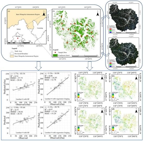
2.1. Study Area

The Wangyedian forest farm is located in Chifeng City (longitude 118°09′~118°30′E, latitude 41°21′~41°39′N), eastern Inner Mongolia Autonomous Region, China (Figure 1). The study area covers an area of 25,958 ha, with an elevation ranging from 800 to 1890 m. The study area is characterized by mid-temperate continental monsoon climate, with an annual average temperature of 4.2 °C and a frost-free period of 117 days. The annual precipitation of Wangyedian forest farm is 400~600 mm [9]. As the main forest type, coniferous forests account for more than 40% of the total area of Wangyedian [42], and the main species include Chinese pine (Pinus tabuliformis), larch (Larix principis-rupprechtii and Larix ologensis), and Scots pine (Pinus sylvestris). As one of the largest plantation forests providing timber in northern China, the total live-standing timber in Wangyedian reaches 1.28 million m³ [43].

2.2. Field Measurement of AGB

The forest survey database in Wangyedian forest farm was used to extract the scope of the coniferous forest. The study area was divided into 22 rectangular sampling areas with a spacing of 4 km. Within the extent of coniferous forest in each rectangular sampling area, a cluster representing the average condition of the forest was laid out, and the cluster consisted of a central plot and three peripheral plots. The central plots were first determined, then the other three plots were determined at 0°, 120°, and 240° directions at 0.5 km intervals, respectively, and, finally, the locations of some sample plots were adjusted according to the actual situation. Finally, 88 sample plots with the size of 25 m × 25 m were surveyed in the Wangyedian forest farm (Figure 1b).

The field survey was carried out in August and September 2019. A real-time kinematic global navigation satellite system (RTK GNSS) was used to determine the location and scope of each sample plot. The individual trees in the sample plots with the diameter at breast height (DBH) greater than 5 cm were marked and selected, and the tree height, DBH, and crown width of each tree were measured. The main tree species and environmental factors of the sample plots were also recorded. The allometric growth equations for AGB calculation used in the study were launched by the National Forestry and Grassland Administration of China (http://www.forestry.gov.cn/ (accessed on 19 July 2022)). The AGB values of individual trees were calculated and summarized into plot-level results and then converted into the hectare-level.

In Wangyedian forest farm, a total of 88 sample plots composed of three tree species, which were Chinese pine, larch, and Scots pine, were investigated. The AGB values in the study area ranged from 24.56 to 459.62 t/ha. The mean value, standard deviation, and coefficient of variation of all the sample plots were 127.46 t/ha, 58.01 t/ha, and 45.5%, respectively. As the main tree species, the mean AGB values of larch and Chinese pine were 115.95 t/ha and 138.29 t/ha, respectively, and the standard deviation of the AGB values of larch and Chinese pine are both lower than that of the total sample (

Table 1. Statistical results of measured AGB in Wangyedian forest farm.

Tree Species	Number	Value Range (t/ha)	Mean (t/ha)	Standard Deviation (t/ha)	Coefficient of Variation (%)
Larch	41	24.56–207.17	115.95	49.14	42.3
Chinese pine	45	28.48–459.62	138.29	64.63	46.7
Scots pine	2	91.04–148.38	119.71	40.55	33.9
Total	88	24.56–459.62	127.46	58.01	45.5

).

2.3. Landsat Images Preprocessing

As the continuation of Landsat 8, Landsat 9 carries the Operational Land Imager 2 (OLI-2) and Thermal Infrared Sensor 2 (TIRS-2) [27]. The OLI-2 will provide observations of the land surface with improved radiometric precision in the visible, near-infrared, and short-wave infrared bands [44], and TIRS-2 of Landsat 9 will measure thermal infrared radiation or heat from the land surface with better performance in both bands than Landsat 8 [45,46]. The spectral band information of Landsat 8 and Landsat 9 maintains a high degree of consistency, which can effectively provide continuous observations (

Table 2. Band information of the Landsat 8 and Landsat 9 used in the study.

Spectral Bands	Wavelength Range (nm)		Spatial Resolution (m)
	Landsat 8/OLI-1	Landsat 9/OLI-2
Band 1—Coastal	435–451	435–450	30
Band 2—Blue	452–512	452–512	30
Band 3—Green	533–590	532–589	30
Band 4—Red	636–673	636–672	30
Band 5—NIR	851–879	850–879	30
Band 6—SWIR 1	1566–1651	1565–1651	30
Band 7—SWIR 2	2107–2294	2105–2294	30
Band 8—Panchromatic	504–676	503–675	15
Band 9—Cirrus	1363–1384	1363–1384	30
	Landsat 8/TIRS-1	Landsat 9/TIRS-2
Band 10—TIRS 1	10.60–11.18	10.45–11.20	100
Band 11—TIRS 2	11.51–12.50	11.58–12.50	100

) [27]. The revisit period of Landsat 9 is 16 days, which is consistent with Landsat 8; however, with an 8-day interval from Landsat 8, this results in a reduced observation period of 8 days for the Landsat series of satellites on Earth [27,47].

A Landsat 8 image dated 5 December 2021 and a Landsat 9 image dated 12 November 2021 covering the Wangyedian forest farm were acquired from the United States Geological Survey (USGS) website (http://glovis.usgs.gov/ (accessed on 19 July 2022)). The cloudiness of acquired images was less than 5%, and the images were T1-level, which had been system-radiation-corrected and geometric-corrected [27,48]. ENVI 5.3 was used for image preprocessing, which were radiation calibration and atmospheric correction, and the pixel values were finally converted into spectral reflectance. Further, Band 1 to Band 7 of Landsat 8 and Landsat 9 were selected for comparison of the AGB modeling and estimation.

2.4. Extraction and Selection of Feature Variables

Feature variables are the basis for AGB modeling and estimation, and reasonable variables can improve the estimation accuracy and interpretability of the model [9]. Commonly used feature variables for AGB estimation include spectral variables, texture features, and topographic factors [31]. Spectral variables mainly consist of band reflectance and vegetation index. The vegetation index is a valid measure of surface vegetation condition that can be formed by combining bands based on spectral characteristics. Vegetation indices can be effectively used to evaluate the growth status of vegetation and have been widely used for land cover change monitoring, deforestation, and AGB estimation [49,50]. Commonly used vegetation indices, including normalized difference vegetation index (NDVI), red–green vegetation index (RGVI), atmospherically resistant vegetation index (ARVI), enhanced vegetation index (EVI), visible atmospherically resistant index (VARI), soil-adjusted vegetation index (SAVI), and modified soil-adjusted vegetation index (MSAVI), were calculated in the study [51,52,53,54,55,56].

Remote sensing images contain abundant texture information, which is very effective to distinguish objects with similar spectral characteristics [57]. The gray level co-occurrence matrix (GLCM) [58,59] was used to extract eight texture features with the window size of 3 × 3, 5 × 5, 7 × 7, and 9 × 9 in the study. To reduce the dimension and redundancy, principal component analysis (PCA) [60] was used to refine the texture information, and components containing at least 90% of texture information in each band were retained. In addition, topographic factors can also affect vegetation growth and forest AGB distribution [9,61]. The elevation, slope, and aspect in Wangyedian forest farm were extracted in this study (

Table 3. List of feature variables used in this study.

Variable Type	Feature Variable	Reference
Spectral variable	Band reflectance (Band i, i = 1, 2, …7)	[43]
	Normalized difference vegetation index (NDVI)	[51]
	Red–green vegetation index (RGVI)	[52]
	Atmospherically resistant vegetation index (ARVI)	[52]
	Enhanced vegetation index (EVI)	[53]
	Visible atmospherically resistant index (VARI)	[54]
	Soil-adjusted vegetation index (SAVI)	[55]
	Modified soil-adjusted vegetation index (MSAVI)	[56]
Texture feature	Mean	[59]
	Variance	[59]
	Homogeneity	[59]
	Contrast	[59]
	Dissimilarity	[59]
	Entropy	[59]
	Second moment	[59]
	Correlation	[59]
Topographic factor	Elevation	[9]
	Slope	[9]
	Aspect	[9]

).

An excessive number of variables involved in modeling may reduce the operational efficiency and interpretability of the model. In addition, selecting variables that are more closely related to the response variable for modeling can effectively increase the estimation accuracy [31,62]. Therefore, it is crucial to screen the variables properly before conducting AGB modeling. Due to the complexity of forest ecosystems, a commonly used linear method, such as linear stepwise regression (LSR), may not be sufficient to accurately describe the relationship between remotely sensed feature variables and AGB [9,30]. Importance assessment is a nonlinear variable evaluation method based on the random forest algorithm that can measure the magnitude of variables’ contribution to AGB modeling and finally achieve variable selection by ranking the relative importance of variables. Importance assessment has been effectively applied to efficient variable selection before LAI, GSV, and AGB modeling and estimation [34,43].

In our study, the relative importance of all the feature variables was calculated and ranked. The increase in mean squared error (%IncMSE) was used to define the relative importance of all variables, and, the larger the value, the higher the importance of the variable [34]. Further, the variables with the smallest RMSE were finally determined based on the RMSE change of the model. The best variable combination was ultimately used to construct the nonparametric models for AGB estimation. To verify the validity of the nonlinear variable selection method, Pearson correlation coefficient was also used to evaluate the linear relationship between the variables and AGB. Linear stepwise regression was used to screen variables to build the multiple linear regression for AGB estimation and comparison.

2.5. Model Development and Assessment

2.5.1. Parametric and Nonparametric Models

As a representative of parametric models, multiple linear regression (MLR) has concise expressions and is easy to implement. MLR can quantitatively measure the relationship between multiple variables and response variable, which has been widely used for estimation of forest parameters [63]. The general expression of MLR used for AGB estimation is shown in Equation (1).

$$Y={\beta }_1{X}_1+{\beta }_2{X}_2+{\beta }_3{X}_3+\dots +{\beta }_n{X}_n+C+e$$

(1)

where Y is the predicted AGB values,$X_1$,$X_2$,$X_3$…$X_n$ are the feature variables, ${\beta }_1,{\beta }_2,{\beta }_3\dots {\beta }_n$ are the regression coefficients, C is the constant, and $e$ is the residual error.

MLR assumes that there is a highly linear relationship between feature variables and AGB, but this may be restricted in complex forest conditions [30]. Nonparametric models do not require any assumptions about the distribution of the data and can describe complex nonlinear relationships, which has great potential for estimating forest parameters [28]. In our study, the nonparametric models, which were SVM, BPNN, and RF, were conducted for AGB estimation. SVM is a supervised learning-based machine learning algorithm that has been widely used in statistical classification as well as regression analysis. SVM can realize nonlinear classification and regressions through kernel method, and a variety of kernel functions are suitable for different complex scenarios. The SVM regressions based on radial basis function, Gaussian function, and exponential kernel function were established in our study. In addition, the penalty coefficient (cost) and kernel function parameter (gamma) were the main parameters of SVM, and the kernel function and the parameter group with the minimum error were determined for AGB estimation [33]. BPNN is a multi-layer feed-forward neural network with strong nonlinear mapping capability. BPNN does not need to determine the mathematical equations of the mapping relationship in advance, and it can obtain satisfactory estimation results by its own training [64]. RF is an ensemble learning algorithm that makes predictions by building a large number of decision trees. RF is easy to understand and insensitive to noise and has been widely used for land type identification and forest parameter estimation. The ntrees (number of regression trees) and mtry (the number of nodes) are the basic parameters of RF [34]. The R package “randomForest” was used for RF model building in the study [65].

2.5.2. Regression Kriging

The kriging method is a geostatistical method for interpolating and predicting stochastic processes based on covariance functions, which can achieve best linear unbiased prediction (BLUP) in a given stochastic process [66]. Regression kriging (RK) is a hybrid geostatistical method with powerful spatial prediction capability that has been proven to be a very reliable and accurate interpolation method. It combines regression models with the kriging of residuals for obtaining more accurate estimates [36,37]. Regression kriging interpolates the residuals obtained from the predictions of the original model and the measured values and then superimposes the predictions of the original model to obtain the new predictions. Regression kriging takes into account spatial autocorrelation and spatial heterogeneity and can correct the original estimation results, which has great potential for soil carbon, precipitation, and air pollution prediction [38,39].

In this study, the optimal model among the parametric and nonparametric models is used in the regression kriging process for AGB trend prediction, and ordinary kriging is used for interpolation of the residuals. The trend prediction and residuals are then superimposed to obtain the residual-corrected AGB spatial distribution prediction. The unvisited locations ${\widehat{z}}_{RK}\left(s_0\right)$ were predicted by summing the predicted trend and residuals:

$${\widehat{z}}_{RK}\left(s_0\right)={\displaystyle \sum }_{k=0}^p{\widehat{\beta }}_k{q}_k\left(s_0\right)+{\displaystyle \sum }_{i=1}^n{\lambda }_{i}e\left(s_i\right)$$

(2)

where ${\widehat{\beta }}_k$ is the estimated trend model coefficients, $q_k\left(s_0\right)$ is the predictive variables at location $s_0$, p is the number of auxiliary variables, $e\left(s_i\right)$ is the residual of the regression model at site $s_i$,${\mathsf{\lambda }}_i$is the kriging weight determined by the spatial autocorrelation structure of the residual, and n is the number of known points.

The kriging regressions based on optimal model among the parametric and nonparametric models were built to compare the validity for AGB estimation in Wangyedian forest farm.

2.5.3. Model Accuracy Assessment

The sample plots were randomly divided into the training set (70%, for model training) and the testing set (30%, for independent validation). The coefficient of determination (R²), root mean square error (RMSE), and mean absolute error (MAE) [67] between the predicted AGB values and observed AGB values were calculated to evaluate the model performance with the testing set. The higher R² means that the observed values and predicted values of the model have a better fitting effect, while lower RMSE, and MAE indicate that the model achieves lower estimation error.

$${\mathrm{R}}^2=1-\frac{{\sum }_{i=1}^n{(y_i-{\widehat{y}}_i)}^2}{{\sum }_{i=1}^n{(y_i-\overline{y})}^2}$$

(3)

$$\mathrm{RMSE}=\sqrt{\frac{{\sum }_{i=1}^n{({\widehat{y}}_i-y_i)}^2}{n}}$$

(4)

$$\mathrm{MAE}=\frac{1}{n}{\displaystyle \sum }_{i=1}^N\left|{\widehat{y}}_i-y_i\right|$$

(5)

where $y_i$ is the observed AGB values, ${\widehat{y}}_i$is the predicted values based on the estimation models, $\overline{y}$ is the mean of all the observed AGB values, and $n$ is the sample size. All the models and calculations were carried out using R 4.2.0 software.

3. Results

3.1. Band Analysis for Landsat 8 and Landsat 9 Images

Band 1 to Band 7 of the Landsat 8 and Landsat 9 images covering Wangyedian were used to analyze the similarity of band information. All the bands maintained a high degree of uniformity, with positive correlation coefficients ranging from 0.77 to 0.89 (p < 0.01). Among them, the correlation coefficients of the RED, NID, and SWIR bands all exceed 0.85, indicating that the band information of Landsat 8 and Landsat 9 was significantly correlated (Figure 2).

In addition, the means and standard deviations of Band 1 to Band 5 of Landsat 8 were smaller than those of Landsat 9 but larger for Band 6 and Band 7. However, the coefficients of variation of Band 1 to Band 5 of Landsat 8 were smaller than those of Landsat 9. In general, the band values of both Landsat 8 and Landsat 9 were similar, and Landsat 9 has the potential to succeed Landsat 8 for acquiring spectral information on vegetation on the land surface (

Table 4. Statistical eigenvalues of bands of Landsat 8 and Landsat 9 in Wangyedian.

Bands	Landsat 8			Landsat 9			Correlation Coefficient
	Mean	Standard Deviation	Coefficient of Variation (%)	Mean	Standard Deviation	Coefficient of Variation (%)
B1	0.10	0.13	127.21	0.23	0.24	104.29	0.77
B2	0.09	0.13	135.17	0.21	0.23	108.53	0.79
B3	0.11	0.13	120.85	0.23	0.24	104.37	0.82
B4	0.13	0.14	107.60	0.24	0.24	99.75	0.85
B5	0.19	0.13	69.27	0.29	0.21	74.41	0.89
B6	0.14	0.11	78.69	0.09	0.06	64.21	0.85
B7	0.11	0.08	78.20	0.07	0.04	61.17	0.87

).

3.2. Correlation and Importance Analysis

Pearson correlation analysis was conducted to test the linear relationship between feature variables and AGB, and the correlation coefficients between the feature variables of Landsat 8 and AGB were similar to those of Landsat 9. The spectral reflectance of all the bands remained negatively correlated with the AGB, and the correlation coefficients of Landsat 9 were slightly higher than those of Landsat 8. For both Landsat 8 and Landsat 9, the correlation coefficient of Band 6 was the highest among all the feature variables.

However, the relative importance of the feature variables from the two data sources behaved slightly differently. Elevation and ARVI are the variables with the highest ranking of importance for Landsat 8 and Landsat 9, respectively. For Landsat 8, the texture features achieved a higher correlation overall; however, the vegetation index and band reflectance were ranked higher in importance in Landsat 9 (Figure 3).

3.3. Comparison of Original AGB Estimation Results

The MLR, SVM, BPNN, and RF models were conducted for AGB estimation using the Landsat 8 and Landsat 9 images in Wangyedian (Figure 4). The MLR, SVM, and BPNN performed similarly; however, RF achieved the highest R² and the lowest RMSE with both data sources. For Landsat 8, the RMSE of RF decreased by 15.8%, 6.5%, and 10.9% compared to MLR, SVM, and BPNN, respectively, while, for Landsat 9, it was 16.2%, 6.7%, and 12.5%, respectively. In addition, for Landsat 8 and Landsat 9, all the models performed similarly; however, Landsat 9 achieved the lowest RMSE of 36.61 t/ha based on the RF model, with a reduction of 3% compared to Landsat 8.

3.4. Regression Kriging for AGB Estimation

As the best original estimation model, the random forest model was used to predict the trend of AGB, and ordinary kriging based on the Gaussian kernel function was used for interpolation of the residuals. The overlay result of the AGB prediction and interpolation of the residuals was regarded as the new AGB predictions, and the scatter plots of the new AGB predictions against the observed AGB values were presented in Figure 5.

The estimation accuracy of regression kriging was greatly improved compared to the original RF model. After overlaying the residuals, the coefficients of determination of the models both exceed 0.8. For Landsat 8, the RMSE of regression kriging was reduced by 55.4% compared to RF, while, for Landsat 9, it was 51.1%. In addition, the results of AGB estimation based on Landsat 8 and regression kriging were slightly better than Landsat 9.

3.5. Spatial Distribution of AGB in Wangyedian

Random forest and regression kriging were used for mapping the spatial distribution of AGB in Wangyedian (Figure 6), and Landsat 8 was used for comparison with Landsat 9 for AGB mapping. Overall, the spatial distributions of AGB obtained by Landsat 8 and Landsat 9 were similar. The mean values of AGB obtained from the random forest of Landsat 8 and Landsat 9 were 116.2 t/ha and 107.7 t/ha, while the results obtained by regression kriging were 121.7 t/ha and 112.6 t/ha, which are closer to the measured values. Compared with random forest regression, the range of AGB predicted by kriging regression has also been expanded. The higher AGB values were mainly distributed in the western and northwestern regions; however, the northern and southwestern regions had relatively low AGB values, and human activities led to relatively low AGB values in the central region. The standard deviations of the AGB spatial distributions obtained based on the random forest model using Landsat 8 and Landsat 9 are 13.7 t/ha and 16.3 t/ha, and for regression kriging are 23.4 t/ha and 24.7 t/ha, respectively, indicating that regression kriging can reduce the homogeneity of the estimation results and enhance the local AGB estimation. In addition, the regression kriging method resulted in a significant improvement in AGB mapping, and the overall distribution was more reasonable and generally consistent with the actual forest distribution in Wangyedian.

4. Discussion

4.1. Comparison of AGB Estimation Models

Parametric and non-parametric models are proven to be effective for forest AGB estimation [28]. Parametric models are simple in form and easy to implement and are convenient and effective in small samples and simple forest structures. Non-parametric models, especially machine learning models, can maintain superior performance in complex forest conditions [30,35]. In our study, all the nonparametric models, including SVM, BPNN, and RF, achieved higher AGB accuracy than MLR overall. Among all the models, RF achieved the lowest RMSE of 37.75 t/ha and 36.61 t/ha using Landsat 8 and Landsat 9, which slightly lowered the RMSE obtained by Jiang et al. (2021) [43].

Regression kriging can effectively reduce the overestimation and underestimation of AGB estimates by analyzing the spatial distribution patterns, such as location and distance of the samples [37]. The regression kriging based on a linear model using Landsat 8 images was established for forest AGB estimation in subtropical China by Li et al. (2020) [38], resulting in a significant reduction in RMSE compared to the original linear model. However, the effectiveness of regression kriging based on nonparametric models, especially machine learning, in forest AGB estimation still needs further verification. RF was the optimal AGB trend prediction model in our study, which was used in combination with kriging regression for AGB estimation, and satisfactory estimation results were obtained. For Landsat 8 and Landsat 9, the RMSE of regression kriging was reduced by 55.4% and 51.1% compared to RF, respectively, which greatly reduced the overestimation and underestimation of AGB. Moran’s index was used to assess the spatial autocorrelation of the residuals obtained by RF. The Moran’s index of residuals obtained from RF using Landsat 8 was 0.41 (p < 0.05), larger than Landsat 9 at 0.37 (p < 0.05), indicating that there is significant spatial auto-correlation within the residuals obtained by RF, and the spatial aggregation effect of the residuals obtained by Landsat 8 was higher than Landsat 9. In addition, the range of AGB spatial distribution estimated by kriging regressions based on Landsat 8 and Landsat 9 increased by 25.5% and 25.1%, respectively, over the original RF, which can describe the differences in local AGB distribution more carefully.Regression kriging has been successfully applied to soil organic carbon estimation, precipitation, and mineral prediction [37,68]. However, the spatial distribution of AGB is influenced by various factors, such as forest type, tree species, and climate [69,70], which can directly lead to spatial heterogeneity in the distribution of AGB. Considering more covariates, such as land surface temperature, soil moisture, climate surfaces, and topographic data, has the potential to further improve the accuracy of AGB estimation [43,71]. In addition, co-kriging has been shown to be effective for estimating the precipitation and soil clay content [43,71,72,73], but the validity in forest AGB still needs further validation in the future.

4.2. Limitations and Prospection

Uncertainties from estimation models, forest types, data sources, and other factors may significantly affect the estimation accuracy of forest AGB [30,53]. Parametric and nonparametric models are popular methods for forest AGB estimation, but the estimation process still suffers from uncertain overestimation and underestimation [43,74]. In this study, the residuals caused by the original RF were interpolated using kriging and superimposed with the predicted trend to reduce estimation errors. The regression kriging estimates finally showed a major improvement in accuracy compared to the original RF, with a 55.4% and 51.1% reduction in RMSE, respectively. In addition, Li et al. [38] demonstrated that the validity of different semi-variance functions was inconsistent for different forest types during the use of regression kriging. The main tree species in Wangyedian forest are Chinese pine and larch, and, since both are planted coniferous forests, this results in most of the regional vegetation having similar spectral characteristics. The Gaussian function was used as semi-variance functions in this study for ordinary kriging interpolation construction, and satisfactory estimation results were achieved. Moreover, the RMSE of RF was reduced by 15.8% and 16.2% compared to MLR for Landsat 8 and Landsat 9, respectively, indicating that the nonparametric model combined with the regression kriging model has more potential than MLR for AGB estimation.

Landsat 8 is one of the most commonly used optical data sources and has been proven to be effective for forest parameter estimation [44,45]. However, as the continuation and inheritance, Landsat 9 needs to be further validated for forest AGB estimation. To explore the usability and validity of Landsat 9, Landsat 8 and Landsat 9 were used as data sources for spectral information comparison and AGB estimation in Wangyedian. The correlation coefficients between Landsat 8 and AGB feature variables were similar to those of Landsat 9, with Band 6 (short-wave infrared) showing the highest correlation coefficients with AGB. Overall, the AGB estimates obtained based on Landsat 8 and Landsat 9 were similar, indicating that Landsat 9 has the same potential for forest resource monitoring as Landsat 8. However, the relative importance of the feature variables from the two data sources and the performance of the estimation results are slightly different, which may be due to the timing of remote sensing image acquisition, differences in cloud coverage, and other factors. Further, for both data sources, RF achieved the lowest RMSE of 37.75 t/ha and 36.61 t/ha among all the estimation models, respectively. Moreover, since Landsat 8 and Landsat 9 are optical data, they can only obtain information on the forest canopy surface, which still suffers from saturation [27,75]. Combining Landsat 9 data with LiDAR or other data sources that can penetrate the canopy and obtain information on the vertical structure of the forest for forest parameter estimation is an effective way to relieve this problem [11,29]. In addition, a Landsat 9 image dated November 2021 was acquired to estimate AGB in Wangyedian, which was almost the earliest Landsat 9 data that can be obtained, and there is a time difference between the Landsat images used in the study and the field measurement of AGB, but the effect of the time difference on the AGB estimate is weak in our study due to the study area being located in northern China at a high latitude with a mean annual temperature of 4.2 °C, resulting in slow tree growth.

The red-edge bands of Sentinel-2 are hypersensitive to chlorophyll changes in the forest canopy and have the potential to mitigate saturation in forest parameter estimation and thus obtain satisfactory estimation accuracy [24]. However, continuous forest monitoring is restricted by the limited time series of the Sentinel-2 data. Landsat series data are still one of the mainstream promising data sources; however, data acquisition and processing of large areas can greatly affect the efficiency of forest survey and monitoring [76,77]. Google Earth Engine (GEE) is an open-source cloud platform that contains massive remote sensing data and superior online computing power. GEE can efficiently access and process remote sensing data over large areas and has been widely used for land cover change detection, forest resource monitoring, and climate change prediction [78]. At present, Landsat 9 has been integrated in GEE, which is extremely meaningful for acquiring and processing Landsat images of long time series. In future research, the GEE cloud platform can be used to acquire and process remote sensing images with higher spatial resolution to achieve high-precision estimation and mapping of forest parameters in large areas with long time series, which is essential for efficient forest resource monitoring [79,80].

5. Conclusions

Forest AGB plays a crucial role in measuring forest growth, health, and in evaluating forest ecosystem service functions. This paper developed a regression kriging method for improving AGB estimation and mapping in Wangyedian forest farm, northern China. Multiple parametric and nonparametric models were used to estimate the trend of AGB. Landsat 8 and Landsat 9 images covering the study area were used as data sources to extract remote sensing variables, modeling, and comparison. The results demonstrated that: (1) the band information of Landsat 8 and Landsat 9 remain highly similar and achieve similar AGB estimation results, and (2) the non-parametric models for AGB estimation were better than MLR overall, with RF performing the best. However, regression kriging greatly improved the AGB estimation, reducing the RMSE based on Landsat 8 and Landsat 9 by 55.4% and 55.1%, respectively. In addition, the range of the spatial distribution of AGB obtained by regression kriging was expanded, which is beneficial to describe the local AGB distribution more carefully. To conclude, by combining regression kriging with Landsat 8 and Landsat 9 images, the spatial distribution of forest AGB can be effectively estimated and mapped, providing a reference for dynamic monitoring and management of forest resources.

References

1. Zhang, R.; Zhou, X.; Ouyang, Z.; Avitabile, V.; Qi, J.; Chen, J.; Giannico, V. Estimating aboveground biomass in subtropical forests of China by integrating multisource remote sensing and ground data. Remote Sens. Environ. 2019, 232, 111341. [Google Scholar] [CrossRef]
2. Tsogt, K.; Lin, C. A flexible modeling of irregular diameter structure for the volume estimation of forest stands. J. For. Res. 2014, 19, 1–11. [Google Scholar] [CrossRef]
3. Xiao, J.; Chevallier, F.; Gomez, C.; Guanter, L.; Hicke, J.A.; Huete, A.R.; Ichii, K.; Ni, W.; Pang, Y.; Rahman, A.F.; et al. Remote sensing of the terrestrial carbon cycle: A review of advances over 50 years. Remote Sens. Environ. 2019, 233, 111383. [Google Scholar] [CrossRef]
4. Gower, S.T. Patterns and mechanisms of the forest carbon cycle. Ann. Rev. Environ. Resour. 2003, 28, 169–204. [Google Scholar] [CrossRef]
5. Tang, X.; Fehrmann, L.; Guan, F.; Forrester, D.I.; Guisasola, R.; Kleinn, C. Inventory-based estimation of forest biomass in Shitai County, China: A comparison of five methods. Ann. For. Res. 2016, 59, 269–280. [Google Scholar] [CrossRef] [Green Version]
6. Federici, S.; Tubiello, F.N.; Salvatore, M.; Jacobs, H.; Schmidhuber, J. New estimates of CO2 forest emissions and removals: 1990–2015. For. Ecol. Manag. 2015, 352, 89–98. [Google Scholar] [CrossRef] [Green Version]
7. Lin, C.; Thomson, G.; Popescu, S. An IPCC-Compliant Technique for Forest Carbon Stock Assessment Using Airborne LiDAR-Derived Tree Metrics and Competition Index. Remote Sens. 2016, 8, 528. [Google Scholar] [CrossRef] [Green Version]
8. Di Cosmo, L.; Gasparini, P.; Tabacchi, G. A national-scale, stand-level model to predict total above-ground tree biomass from growing stock volume. For. Ecol. Manag. 2016, 361, 269–276. [Google Scholar] [CrossRef]
9. Jiang, F.; Kutia, M.; Sarkissian, A.J.; Lin, H.; Long, J.; Sun, H.; Wang, G. Estimating the Growing Stem Volume of Coniferous Plantations Based on Random Forest Using an Optimized Variable Selection Method. Sensors 2020, 20, 7248. [Google Scholar] [CrossRef]
10. Mahdianpari, M.; Salehi, B.; Mohammadimanesh, F.; Motagh, M. Random forest wetland classification using ALOS-2 L-band, RADARSAT-2 C-band, and TerraSAR-X imagery. ISPRS J. Photogramm. Remote Sens. 2017, 130, 13–31. [Google Scholar] [CrossRef]
11. Shao, G.; Stark, S.C.; de Almeida, D.R.A.; Smith, M.N. Towards high throughput assessment of canopy dynamics: The estimation of leaf area structure in Amazonian forests with multitemporal multi-sensor airborne lidar. Remote Sens. Environ. 2019, 221, 1–13. [Google Scholar] [CrossRef]
12. Ehlers, D.; Wang, C.; Coulston, J.; Zhang, Y.; Pavelsky, T.; Frankenberg, E.; Woodcock, C.; Song, C. Mapping Forest Aboveground Biomass Using Multisource Remotely Sensed Data. Remote Sens. 2022, 14, 1115. [Google Scholar] [CrossRef]
13. Beaudoin, A.; Hall, R.J.; Castilla, G.; Filiatrault, M.; Villemaire, P.; Skakun, R.; Guindon, L. Improved k-NN Mapping of Forest Attributes in Northern Canada Using Spaceborne L-Band SAR, Multispectral and LiDAR Data. Remote Sens. 2022, 14, 1181. [Google Scholar] [CrossRef]
14. Entwistle, N.; Heritage, G.; Milan, D. Recent remote sensing applications for hydro and morphodynamic monitoring and modelling. Earth Surf. Process. Landforms. 2018, 43, 2283–2291. [Google Scholar] [CrossRef] [Green Version]
15. Thiel, C.; Schmullius, C. The potential of ALOS PALSAR backscatter and InSAR coherence for forest growing stock volume estimation in Central Siberia. Remote Sens. Environ. 2016, 173, 258–273. [Google Scholar] [CrossRef]
16. Antonarakis, A.S.; Richards, K.S.; Brasington, J.; Bithell, M. Leafless roughness of complex tree morphology using terrestrial lidar. Water Resour. Res. 2009, 45, W10401. [Google Scholar] [CrossRef] [Green Version]
17. Wu, J.; Yao, W.; Choi, S.; Park, T.; Myneni, R.B. A Comparative Study of Predicting DBH and Stem Volume of Individual Trees in a Temperate Forest Using Airborne Waveform LiDAR. IEEE Geosci. Remote Sens. Lett. 2015, 12, 2267–2271. [Google Scholar] [CrossRef]
18. Labrecque, S.; Fournier, R.A.; Luther, J.E.; Piercey, D. A comparison of four methods to map biomass from Landsat-TM and inventory data in western Newfoundland. For. Ecol. Manag. 2006, 226, 129–144. [Google Scholar] [CrossRef]
19. Amiro, B.D.; Chen, J.M. Forest-fire-scar aging using SPOT-VEGETATION for Canadian ecoregions. Can. J. For. Res. 2003, 33, 1116–1125. [Google Scholar] [CrossRef]
20. Jiang, F.; Deng, M.; Long, Y.; Sun, H. Spatial Pattern and Dynamic Change of Vegetation Greenness from 2001 to 2020 in Tibet, China. Front. Plant Sci. 2022, 13, 892625. [Google Scholar] [CrossRef]
21. Wilson, K.L.; Wong, M.C.; Devred, E. Comparing Sentinel-2 and WorldView-3 Imagery for Coastal Bottom Habitat Mapping in Atlantic Canada. Remote Sens. 2022, 14, 1254. [Google Scholar] [CrossRef]
22. Chaozong, X.; Yuxing, Z.; Wei, W. A relief-based forest cover change extraction using GF-1 images. In Proceedings of the 2014 IEEE Geoscience and Remote Sensing Symposium, Quebec City, QC, Canada, 13–18 July 2014; pp. 4212–4215. [Google Scholar] [CrossRef]
23. Lu, D.; Chen, Q.; Wang, G.; Liu, L.; Li, G.; Moran, E. A survey of remote sensing-based aboveground biomass estimation methods in forest ecosystems. Int. J. Digit. Earth 2014, 9, 63–105. [Google Scholar] [CrossRef]
24. Majasalmi, T.; Rautiainen, M. The potential of Sentinel-2 data for estimating biophysical variables in a boreal forest: A simulation study. Remote Sens. Lett. 2016, 7, 427–436. [Google Scholar] [CrossRef]
25. Tomppo, E.O.; Gagliano, C.; De Natale, F.; Katila, M.; McRoberts, R.E. Predicting categorical forest variables using an improved k-Nearest Neighbour estimator and Landsat imagery. Remote Sens. Environ. 2009, 113, 500–517. [Google Scholar] [CrossRef]
26. Phiri, D.; Morgenroth, J. Developments in Landsat Land Cover Classification Methods: A Review. Remote Sens. 2017, 9, 967. [Google Scholar] [CrossRef] [Green Version]
27. Masek, J.G.; Wulder, M.A.; Markham, B.; McCorkel, J.; Crawford, C.J.; Storey, J.; Jenstrom, D.T. Landsat 9: Empowering open science and applications through continuity. Remote Sens. Environ. 2020, 248, 111968. [Google Scholar] [CrossRef]
28. Chirici, G.; Barbati, A.; Corona, P.; Marchetti, M.; Travaglini, D.; Maselli, F.; Bertini, R. Non-parametric and parametric methods using satellite images for estimating growing stock volume in alpine and Mediterranean forest ecosystems. Remote Sens. Environ. 2008, 112, 2686–2700. [Google Scholar] [CrossRef] [Green Version]
29. García-Gutiérrez, J.; Martínez-álvarez, F.; Troncoso, A.; Riquelme, J.C. A comparison of machine learning regression techniques for lidar-derived estimation of forest variables. Neurocomputing 2015, 167, 24–31. [Google Scholar] [CrossRef]
30. Li, Y.; Han, N.; Li, X.; Du, H.; Mao, F.; Cui, L.; Liu, T.; Xing, L. Spatiotemporal Estimation of Bamboo Forest Aboveground Carbon Storage Based on Landsat Data in Zhejiang, China. Remote Sens. 2018, 10, 898. [Google Scholar] [CrossRef]
31. Li, Y.; Li, C.; Li, M.; Liu, Z. Influence of Variable Selection and Forest Type on Forest Aboveground Biomass Estimation Using Machine Learning Algorithms. Forests 2019, 10, 1073. [Google Scholar] [CrossRef] [Green Version]
32. Zhu, Y.; Liu, K.; Liu, L.; Myint, S.W.; Wang, S.; Liu, H.; He, Z. Exploring the Potential of WorldView-2 Red-Edge Band-Based Vegetation Indices for Estimation of Mangrove Leaf Area Index with Machine Learning Algorithms. Remote Sens. 2017, 9, 1060. [Google Scholar] [CrossRef] [Green Version]
33. Lv, D.; Liu, G.; Ou, J.; Wang, S.; Gao, M. Prediction of GPS Satellite Clock Offset Based on an Improved Particle Swarm Algorithm Optimized BP Neural Network. Remote Sens. 2022, 14, 2407. [Google Scholar] [CrossRef]
34. Breiman, L. Random forests. Mach. Learn. 2001, 45, 5–32. [Google Scholar] [CrossRef] [Green Version]
35. Jiang, F.; Smith, A.R.; Kutia, M.; Wang, G.; Liu, H.; Sun, H. A Modified KNN Method for Mapping the Leaf Area Index in Arid and Semi-Arid Areas of China. Remote Sens. 2020, 12, 1884. [Google Scholar] [CrossRef]
36. Hengl, T.; Heuvelink, G.; Stein, A. A generic framework for spatial prediction of soil variables based on regression-kriging. Geoderma 2004, 120, 75–93. [Google Scholar] [CrossRef] [Green Version]
37. Ge, Y.; Liang, Y.; Wang, J.; Zhao, Q.; Liu, S. Upscaling Sensible Heat Fluxes with Area-to-Area Regression Kriging. IEEE Geosci. Remote Sens. Lett. 2015, 12, 656–660. [Google Scholar] [CrossRef]
38. Li, Y.; Li, M.; Liu, Z.; Li, C. Combining Kriging Interpolation to Improve the Accuracy of Forest Aboveground Biomass Estimation using Remote Sensing Data. IEEE Access 2020, 8, 128124–128139. [Google Scholar] [CrossRef]
39. Yu, S.; Ye, Q.; Zhao, Q.; Li, Z.; Zhang, M.; Zhu, H.; Zhao, Z. Effects of Driving Factors on Forest Aboveground Biomass (AGB) in China’s Loess Plateau by Using Spatial Regression Models. Remote Sens. 2022, 14, 2842. [Google Scholar] [CrossRef]
40. Coletti, C.; Ciotoli, G.; Benà, E.; Brattich, E.; Cinelli, G.; Galgaro, A.; Massironi, M.; Mazzoli, C.; Mostacci, D.; Morozzi, P.; et al. The assessment of local geological factors for the construction of a Geogenic Radon Potential map using regression kriging. A case study from the Euganean Hills volcanic district (Italy). Sci. Total Environ. 2022, 808, 152064. [Google Scholar] [CrossRef]
41. Li, W.; Niu, Z.; Gao, S.; Wang, C. Mapping the spatial pattern of temperate forest above ground biomass by integrating airborne lidar with Radarsat-2 imagery via geostatistical models. Lidar. Remote Sens. Environ. Monit. XIV 2014, 9262, 92620S. [Google Scholar] [CrossRef]
42. Xie, Z.; Chen, Y.; Lu, D.; Li, G.; Chen, E. Classification of land cover, forest, and tree species classes with ZiYuan-3 multispectral and stereo data. Remote Sens. 2019, 11, 164. [Google Scholar] [CrossRef] [Green Version]
43. Jiang, F.; Kutia, M.; Ma, K.; Chen, S.; Long, J.; Sun, H. Estimating the aboveground biomass of coniferous forest in Northeast China using spectral variables, land surface temperature and soil moisture. Sci. Total Environ. 2021, 785, 147335. [Google Scholar] [CrossRef] [PubMed]
44. Gross, G.; Helder, D.; Begeman, C.; Leigh, L.; Kaewmanee, M.; Shah, R. Initial Cross-Calibration of Landsat 8 and Landsat 9 Using the Simultaneous Underfly Event. Remote Sens. 2022, 14, 2418. [Google Scholar] [CrossRef]
45. Gerace, A.; Kleynhans, T.; Eon, R.; Montanaro, M. Towards an Operational, Split Window-Derived Surface Temperature Product for the Thermal Infrared Sensors Onboard Landsat 8 and 9. Remote Sens. 2020, 12, 224. [Google Scholar] [CrossRef] [Green Version]
46. Hair, J.H.; Reuter, D.C.; Tonn, S.L.; McCorkel, J.; Simon, A.A.; Djam, M.; Alexander, D.; Ballou, K.; Barclay, R.; Coulter, P.; et al. Landsat 9 thermal infrared sensor2 architecture and design. In Proceedings of the IGARSS 2018 IEEE International Geoscience and Remote Sensing Symposium, Valencia, Spain, 22–27 July 2018. [Google Scholar] [CrossRef]
47. Randy, S. Landsat 9 Satellite Continues Half-Century of Earth Observations: Eyes in the sky serve as a valuable tool for stewardship. BioScience 2022, 72, 226–232. [Google Scholar] [CrossRef]
48. Roy, D.P.; Wulder, M.A.; Loveland, T.R.; Woodcock, C.; Allen, R.G.; Anderson, M.C.; Helder, D.; Irons, J.R.; Johnson, D.M.; Kennedy, R. Landsat-8: Science and product vision for terrestrial global change research. Remote Sens. Environ. 2014, 145, 154–172. [Google Scholar] [CrossRef] [Green Version]
49. Sandholt, I.; Rasmussen, K.; Andersen, J. A simple interpretation of the surface temperature/vegetation index space for assessment of surface moisture status. Remote Sens. Environ. 2002, 79, 213–224. [Google Scholar] [CrossRef]
50. Motohka, T.; Nasahara, K.N.; Oguma, H.; Tsuchida, S. Applicability of Green-Red Vegetation Index for Remote Sensing of Vegetation Phenology. Remote Sens. 2010, 2, 2369–2387. [Google Scholar] [CrossRef]
51. Yuan, F.; Bauer, M.E. Comparison of impervious surface area and normalized difference vegetation index as indicators of surface urban heat island effects in Landsat imagery. Remote Sens. Environ. 2007, 106, 375–386. [Google Scholar] [CrossRef]
52. Jenson, J.R. Introductory digital image processing: A remote sensing perspective. Geocarto Int. 1987, 2, 65. [Google Scholar] [CrossRef]
53. Lu, D. The potential and challenge of remote sensing-based biomass estimation. Int. J. Remote Sens. 2006, 27, 1297–1328. [Google Scholar] [CrossRef]
54. Dong, T.; Liu, J.; Shang, J.; Qian, B.; Ma, B.; Kovacs, J.M.; Walters, D.; Jiao, X.; Geng, X.; Shi, Y. Assessment of red-edge vegetation indices for crop leaf area index estimation. Remote Sens. Environ. 2019, 222, 133–143. [Google Scholar] [CrossRef]
55. Gitelson, A.A.; Viña, A.; Arkebauer, T.J.; Rundquist, D.C.; Keydan, G.; Leavitt, B. Remote estimation of leaf area index and green leaf biomass in maize canopies. Geophys. Res. Lett. 2003, 30, 1248. [Google Scholar] [CrossRef] [Green Version]
56. Qi, J.G.; Chehbouni, A.R.; Huete, A.R.; Kerr, Y.H.; Sorooshian, S. A modified soil adjusted vegetation index. Remote Sens. Environ. 1994, 48, 119–126. [Google Scholar] [CrossRef]
57. He, D.C.; Wang, L. Texture features based on texture spectrum. Pattern Recognit. 1991, 24, 391–399. [Google Scholar] [CrossRef]
58. Baraldi, A.; Parmiggiani, F. Investigation of the textural characteristics associated with gray level cooccurrence matrix statistical parameters. IEEE Trans. Geosci. Remote Sens. 1995, 33, 293–304. [Google Scholar] [CrossRef]
59. Manjunath, B.S.; Ma, W.Y. Texture features for browsing and retrieving of large image data. IEEE Trans. Pattern Anal. Mach. Intell. 2011, 33, 117–128. [Google Scholar] [CrossRef] [Green Version]
60. Jolliffe, I.T. Principal Component Analysis. J. Mark. Res. 2002, 87, 513. [Google Scholar] [CrossRef]
61. Ghorbanzadeh, O.; Blaschke, T.; Gholamnia, K.; Meena, S.R.; Tiede, D.; Aryal, J. Evaluation of Different Machine Learning Methods and Deep-Learning Convolutional Neural Networks for Landslide Detection. Remote Sens. 2019, 11, 196. [Google Scholar] [CrossRef] [Green Version]
62. Jain, A.; Zongker, D. Feature selection: Evaluation, application, and small sample performance. IEEE Trans. Pattern Anal. Mach. Intell. 1997, 19, 153–158. [Google Scholar] [CrossRef] [Green Version]
63. Li, G.; Xie, Z.; Jiang, X.; Lu, D.; Chen, E. Integration of ZiYuan-3 Multispectral and Stereo Data for Modeling Aboveground Biomass of Larch Plantations in North China. Remote Sens. 2019, 11, 2328. [Google Scholar] [CrossRef] [Green Version]
64. Panda, S.S.; Ames, D.P.; Panigrahi, S. Application of Vegetation Indices for Agricultural Crop Yield Prediction Using Neural Network Techniques. Remote Sens. 2010, 2, 673–696. [Google Scholar] [CrossRef] [Green Version]
65. Liaw, A.; Wiener, M. Classification and Regression by randomForest. R News 2002, 2, 18–22. [Google Scholar]
66. Li, Z.; Wang, J.; Tang, H.; Huang, C.; Yang, F.; Chen, B.; Wang, X.; Xin, X.; Ge, Y. Predicting Grassland Leaf Area Index in the Meadow Steppes of Northern China: A Comparative Study of Regression Approaches and Hybrid Geostatistical Methods. Remote Sens. 2016, 8, 632. [Google Scholar] [CrossRef] [Green Version]
67. Willmott, C.J.; Ackleson, S.G.; Davis, R.E.; Feddema, J.J.; Klink, K.M.; Legates, D.R. Statistics for the evaluation and comparison of models. J. Geophys. Res. 1985, 90, 8995. [Google Scholar] [CrossRef] [Green Version]
68. Zhang, Y.; Guo, L.; Chen, Y.; Shi, T.; Luo, M.; Ju, Q.; Zhang, H.; Wang, S. Prediction of Soil Organic Carbon based on Landsat 8 Monthly NDVI Data for the Jianghan Plain in Hubei Province, China. Remote Sens. 2019, 11, 1683. [Google Scholar] [CrossRef] [Green Version]
69. Yu, Y.; Pan, Y.; Yang, X.; Fan, W. Spatial Scale Effect and Correction of Forest Aboveground Biomass Estimation Using Remote Sensing. Remote Sens. 2022, 14, 2828. [Google Scholar] [CrossRef]
70. Pirotti, F.; Laurin, G.V.; Vettore, A.; Masiero, A.; Valentini, R. Small Footprint Full-Waveform Metrics Contribution to the Prediction of Biomass in Tropical Forests. Remote Sens. 2014, 6, 9576–9599. [Google Scholar] [CrossRef] [Green Version]
71. Hu, T.; Zhang, Y.; Su, Y.; Zheng, Y.; Lin, G.; Guo, Q. Mapping the Global Mangrove Forest Aboveground Biomass Using Multisource Remote Sensing Data. Remote Sens. 2020, 12, 1690. [Google Scholar] [CrossRef]
72. Zhang, J.; Xu, J.; Dai, X.; Ruan, H.; Liu, X.; Jing, W. Multi-Source Precipitation Data Merging for Heavy Rainfall Events Based on Cokriging and Machine Learning Methods. Remote Sens. 2022, 14, 1750. [Google Scholar] [CrossRef]
73. Shabou, M.; Mougenot, B.; Chabaane, Z.L.; Walter, C.; Boulet, G.; Aissa, N.B.; Zribi, M. Soil Clay Content Mapping Using a Time Series of Landsat TM Data in Semi-Arid Lands. Remote Sens. 2015, 7, 6059–6078. [Google Scholar] [CrossRef] [Green Version]
74. Brovkina, O.; Novotny, J.; Cienciala, E.; Zemek, F.; Russ, R. Mapping forest aboveground biomass using airborne hyperspectral and LiDAR data in the mountainous conditions of Central Europe. Ecol. Eng. 2017, 100, 219–230. [Google Scholar] [CrossRef]
75. Vuolo, F.; Żółtak, M.; Pipitone, C.; Zappa, L.; Wenng, H.; Immitzer, M.; Weiss, M.; Baret, F.; Atzberger, C. Data Service Platform for Sentinel-2 Surface Reflectance and Value-Added Products: System Use and Examples. Remote Sens. 2016, 8, 938. [Google Scholar] [CrossRef] [Green Version]
76. Myneni, R.; Maggion, S.; Iaquinta, J.; Privette, J.; Gobron, N.; Pinty, B.; Kimes, D.; Verstraete, M.; Williams, D. Optical remote sensing of vegetation: Modeling, caveats, and algorithms. Remote Sens. Environ. 1995, 51, 169–188. [Google Scholar] [CrossRef]
77. Banskota, A.; Kayastha, N.; Falkowski, M.J.; Wulder, M.A.; Froese, R.E.; White, J.C. Forest Monitoring Using Landsat Time Series Data: A Review. Can. J. Remote Sens. 2014, 40, 362–384. [Google Scholar] [CrossRef]
78. Seydi, S.; Akhoondzadeh, M.; Amani, M.; Mahdavi, S. Wildfire Damage Assessment over Australia Using Sentinel-2 Imagery and MODIS Land Cover Product within the Google Earth Engine Cloud Platform. Remote Sens. 2021, 13, 220. [Google Scholar] [CrossRef]
79. Tassi, A.; Vizzari, M. Object-Oriented LULC Classification in Google Earth Engine Combining SNIC, GLCM, and Machine Learning Algorithms. Remote Sens. 2020, 12, 3776. [Google Scholar] [CrossRef]
80. Tamiminia, H.; Salehi, B.; Mahdianpari, M.; Quackenbush, L.; Adeli, S.; Brisco, B. Google Earth Engine for geo-big data applications: A meta-analysis and systematic review. ISPRS J. Photogramm. Remote Sens. 2020, 164, 152–170. [Google Scholar] [CrossRef]
Figure 1. (a) Locations of the study area and (b) distribution of sample plots within the coniferous forest in the Wangyedian forest farm.
Remotesensing 14 05734 g001
Figure 2. The scatter plots of Band 1 to Band 7 of Landsat 8 and Landsat 9 images in Wangyedian.
Remotesensing 14 05734 g002
Figure 3. Correlation coefficient matrix of (a) Landsat 8 variables and (b) Landsat 9 variables; the relative importance ranking of (c) Landsat 8 variables and (d) Landsat 9 variables.
Remotesensing 14 05734 g003
Figure 4. Scatter plots of the predicted AGB against the observed AGB values in Wangyedian using: (a) Landsat 8 and MLR, (b) Landsat 8 and SVM, (c) Landsat 8 and BPNN, (d) Landsat 8 and RF, (e) Landsat 9 and MLR, (f) Landsat 9 and SVM, (g) Landsat 9 and BPNN, and (h) Landsat 9 and RF.
Remotesensing 14 05734 g004
Figure 5. Scatter plots of the predicted AGB by regression kriging against the observed AGB values in Wangyedian using: (a) Landsat 8 and (b) Landsat 9.
Remotesensing 14 05734 g005
Figure 6. Spatial distributions of forest AGB in Wangyedian using (a) the Landsat 8 with RF, (b) the Landsat 8 with regression kriging, (c) the Landsat 9 with RF, and (d) the Landsat 9 with regression kriging.
Remotesensing 14 05734 g006