
Inner Dynamic Detection and Prediction of Water Quality Based on CEEMDAN and GA-SVM Models


1
Key Laboratory of Water Cycle & Related Land Surface Processes, Institute of Geographic Sciences and Natural Resources Research, Chinese Academy of Sciences, Beijing 100101, China
2
University of Chinese Academy of Sciences, Beijing 100049, China
3
State Key Laboratory of Water Resources and Hydropower Engineering Science, Wuhan University, Wuhan 430072, China
4
Key Laboratory of Ecosystem Network Observation and Modeling, Institute of Geographic Sciences and Natural Resources Research, Chinese Academy of Sciences, Beijing 100101, China
*
Author to whom correspondence should be addressed.
Remote Sens. 2022, 14(7), 1714; https://doi.org/10.3390/rs14071714
Submission received: 6 February 2022
/
Revised: 25 March 2022
/
Accepted: 30 March 2022
/
Published: 1 April 2022
(This article belongs to the Special Issue Remote Sensing and Geospatial Approaches for Studying the Environment Affected by Human Activities)
Abstract
:Urban water quality is facing strongly adverse degradation in rapidly developing areas. However, there exists a huge challenge to estimating the inner features and predicting the variation of long-term water quality due to the lack of related monitoring data and the complexity of urban water systems. Fortunately, multi-remote sensing data, such as nighttime light and evapotranspiration (ET), provide scientific data support and reasonably reveal the variation mechanisms. Here, we develop an integrated decomposition-reclassification-prediction method for water quality by integrating the CEEMDN method, the RF method mothed, and the genetic algorithm-support vector machine model (GA-SVM). The degression of the long-term water quality was decomposed and reclassified into three different frequency terms, i.e., high-frequency, low-frequency, and trend terms, to reveal the inner mechanism and dynamics in the CEEMDAN method. The RF method was then used to identify the teleconnection and the significance of the selected driving factors. More importantly, the GA-SVM model was designed with two types of model schemes, which were the data-driven model (GA-SVMd) and the integrated CEEMDAN-GA-SVM model (defined as GA-SVMc model), in order to predict urban water quality. Results revealed that the high-frequency terms for NH3-N and TN had a major contribution to the water quality and were mainly dominated by hydrometeorological factors such as ET, rainfall, and the dynamics of the lake water table. The trend terms revealed that the water quality continuously deteriorated during the study period; the terms were mainly regulated by the land use and land cover (LULC), land metrics, population, and yearly rainfall. The predicting results confirmed that the integrated GA-SVMc model had better performance than single data-driven models (such as the GA-SVM model). Our study supports that the integrated method reveals variation rules in water quality and provides early warning and guidance for reducing the water pollutant concentration.
1. Introduction
Recently, urban water quality degradation has become a considerable restricting factor for achieving the goal of the green development in metropolises, and thus has caused worldwide concern [1,2]. Urbanization rates and the urban built-up area confirm that urban area tends to continuously expand [3] and thus change the structure of the water system, causing potential water pollution [4,5]. For instance, 32% of surface water in China was facing water pollution disasters [6,7]. Waterbody quality strongly varies in time due to uneven development of the urban area; the ongoing drastic change of the effective soil water amounts, nutrient levels, and land use and land cover; and point sources of pollution discharged from residential and industrial sources [8,9]. Thus, accurately detecting the inner dynamics and predicting potential water pollution issues caused by the varied driving factors are the key points to preventing and reducing the degree of water pollution and require immediate attention [10]. Particularly in the urban-rural marginal area, urban expansion has a substantial influence on the hydrology and water environment. Moreover, the high disturbance in the urban has caused more complex hydraulic conditions and more sources of pollutants [11,12].
To detect the inner variation features of the water quality, plenty of methods exist and have provided reasonable results [13,14,15,16,17,18,19,20,21]. However, there also exist some limitations that have restricted the application of these methods. The Mann–Kendall test is mainly used to detect the tendency of time-related data, and thus is widely used for analyzing long-term rainfall, runoff datasets, and water quality [13,15]. However, water quality for urban areas undergoing rapid expansion may not have a long time series of detection data. Moreover, more decomposed features are necessary to analyze the dynamic of water quality. The Fourier transformation (FT) method has also been used to detect the dynamic pattern of time series data; however, the features of stationary and linear processes and priori basis restrict its application for water quality [16]. The wavelet transform (WT) method, which solves the shortage of FT method in the single resolution of short time, is a time-frequency based method and thus is widely used for rainfall, runoff, and water quality transformation [17,18,19,20]. The WT method is suitable for non-stationary signals and is extremely dependent on the wavelet basis function. When the signal-to-noise ratio is small or the data is not linear [21], the denoising effect of WT cannot obtain reasonable results. The empirical mode decomposition (EMD) method has been proposed [22], as the EMD method can compose the non-stationary and non-linear into linearizing and stabilizing series, and the EMD method can select the basis function based on the time scale characteristics of the signals themselves. Furthermore, with the development of other improved EMD methods, such as the complete ensemble empirical mode decomposition with adaptive noise (CEEMDAN) method and ensemble empirical mode decomposition (EEMD), EMD, EEMD, and CEEMDAN have been widely used to decompose time series data of the climatic oscillation, runoff, water quality, and landslides [23,24,25,26,27,28].
Prediction of the variation of water quality also significantly supports improving waterbody deterioration. Several models and information systems have been proposed to predict the variation of water quality and obtain reasonable results. Among these models, physical-based models, i.e., hydrologic-environmental models, have been widely used in urban areas. For example, Joshi et al. [29] used the storm water management model (SWMM) to reduce combined sewer overflows with reasonable cost-effectiveness for sustainable urban drainage systems. The InfoWorks ICM model or the full hydrodynamic (FH) models were widely used for multi-scale catchments in real-time control (RTC) and obtained optimum results [30,31]. The Mike URBAN model contains distributed water systems including combined sewer overflow system and separate stormwater system. More importantly, the Mike URBAN covers two-dimensional overland flow and thus has good performance in urban areas with rapid urbanization and climate change [32]. These models are both supported by rigorous physical theory and are easily acceptable. However, the rigorous physical theory-based models also need high-quality monitoring data to satisfy the accuracy of the model.
However, the rapid expansion of urban areas is always accompanied by drastic changes in the underlying surface, urban pipe networks, hydrological conditions, and water environment conditions. Moreover, all of these changes are not always well monitored or do not have high-quality data available. Therefore, data-driven models, such as machine learning models, have also been used for water quality predictions. Zhi et al. [33] used machine learning models in 236 minimally disturbed watersheds of the US and confirmed that machine learning models can predict results well in data-lacking areas. With the immense and urgent demand for good-quality prediction of water quality variation with the rapid development of urban areas, more machine learning models have been presented and compared. Qiao et al. [34] used 12 machine learning algorithms to evaluate water quality, and both models obtained reasonable results. Compared with the neural network model, Mohammadpour et al. [35] also analyzed the SVM model and artificial neural networks (ANNs), and revealed that the SVM model could obtain better results with limited monitoring data. Recently, a few types of integrated models, which can decompose the data series into more inner sequences and which are then coupled with the machine learning model, were analyzed to evaluate the inner dynamic and provide better modeling performance. For example, the EMD-ANN model and EMD-Auto-Regressive and Moving Average (ARMA) model were integrated to predict runoff, and revealing that the EMD-based integrated model performed better than the single model, i.e., the ANN model and the ARMA model, in the hindcast experiment performed [36]. Yuan et al. [25] integrated the EEMD and Long Short-Term Memory (LSTM) models to forecast daily runoff, and confirmed that the integrated model significantly improved the simulation results compared to the LSTM model. The EEMD and the SVM model also were integrated to predict water quality and landslide displacement, and results revealed that the integrated model increased the prediction accuracy [27,28]. However, some of the EMD-based integrated models were not data-based [27], and some forecast results of the integrated models performed worse than the original models [36].
To evaluate the inner dynamic and achieve better prediction performance of water quality with limited data, this study integrated the CEEMDAN method, the random forest method, and the GA-SVM model. The CEEMDAN method was used to decompose the long-term water quality data; then, the decomposed sequences were reclassified into three sequences according to the variance proportion, i.e., the high-frequency term, the low-frequency term, and the trend term. Furthermore, the RF method was used to identify the importance of the driving data on the water quality series, the high-frequency term, the low-frequency term, and the trend term. More importantly, we then used the GA-SVM model and the identified driving factors of the high-frequency, low-frequency, and trend terms to predict the different terms, which were then coupled to predict the water quality. In contrast, the data-driven model, i.e., the identified driving factors of the water quality series coupled with the GA-SVM model, was set to forecast water quality.
2. Materials and Methods
2.1. The CEEMDAN Method
The complete ensemble empirical mode decomposition with adaptive noise (CEEMDAN) method was developed from empirical mode decomposition (EMD) and ensemble empirical mode decomposition (EEMD) by adding adaptive white noise to suppress the aliasing of the EMD [22,37,38] The CEEMADAN model is an efficient decomposed method for the adaptive decomposition of non-stationary and non-linear data into many intrinsic mode functions (IMF). The main progress is as follows:
Step 1 Define the long-term data xi(t) as the original input signal.
where ε represents a noise coefficient and indicates white noise sequences.
Step 2 Decompose the IMF1. The first decomposed IMF averaged by the EMD method:
The residue is defined as:
Step 3 Decompose the IMF2.
Step 4 Decompose the other IMFs unless the extreme points are less than two. Therefore, the final signal sequences x(t) are decomposed as follows:
In the decomposing process, the IMFs and trend term can extract series terms for the high-frequency to low-frequency and trend terms. In this study, the t-test was used to reclassify the IMFs based on fine-to-coarse reclassification [39].
2.2. Driving Factors Selection and the Relative Importance Analysis
Urban water quality was influenced by many factors due to the complexity of the urban water system [12], such as the heavy variation of LULC, land metrics, rainfall, the human control of the lake water table, multi-point sources, complex rainfall-induced runoff, and non-point pollutants. Therefore, identifying the important driving factors under the condition of limited monitoring data and remote sensing data was the key point to achieving more accurate predictions. Before evaluating the importance of the driving factors, the Pearson method was used to analyze the correlation between the selected factors and to exclude the variables with high correlation. The random forest (RF) method split each partition into a random subset to search for the best feature variable, which produces better overall performance and thus has been widely used for identifying the importance of the driving factors for water quality [40]. Therefore, the RF method was used to identify the importance of the driving factors for the water quality series, the high-frequency term, the low-frequency term, and the trend term.
2.3. GA-SVM Model
The support vector machine (SVM) model is a nonlinear regression and is widely used for predicting hydrological issues and water quality issues. In this study, we used the SVM model to predict the water quality; the input data were divided into training data and test data. Furthermore, the GA imitates biological evolution to approach the best solution of the minimum project [41], and thus was used to search for the best matching kernel function and parameters for the SVM model.
The Nash–Sutcliffe efficiency coefficient (NSE) and the root mean squared error (RMSE) were used to estimate the model performance.
where the ymod and yobs represent the modeled and observed water quality. represents the observed mean of water quality and n represents the number of water quality samplings.
2.4. Experimental Schemes Design
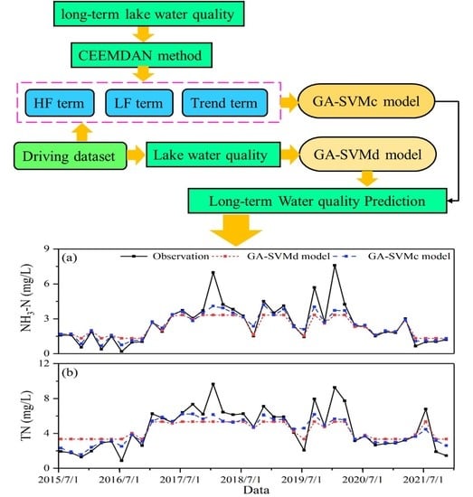
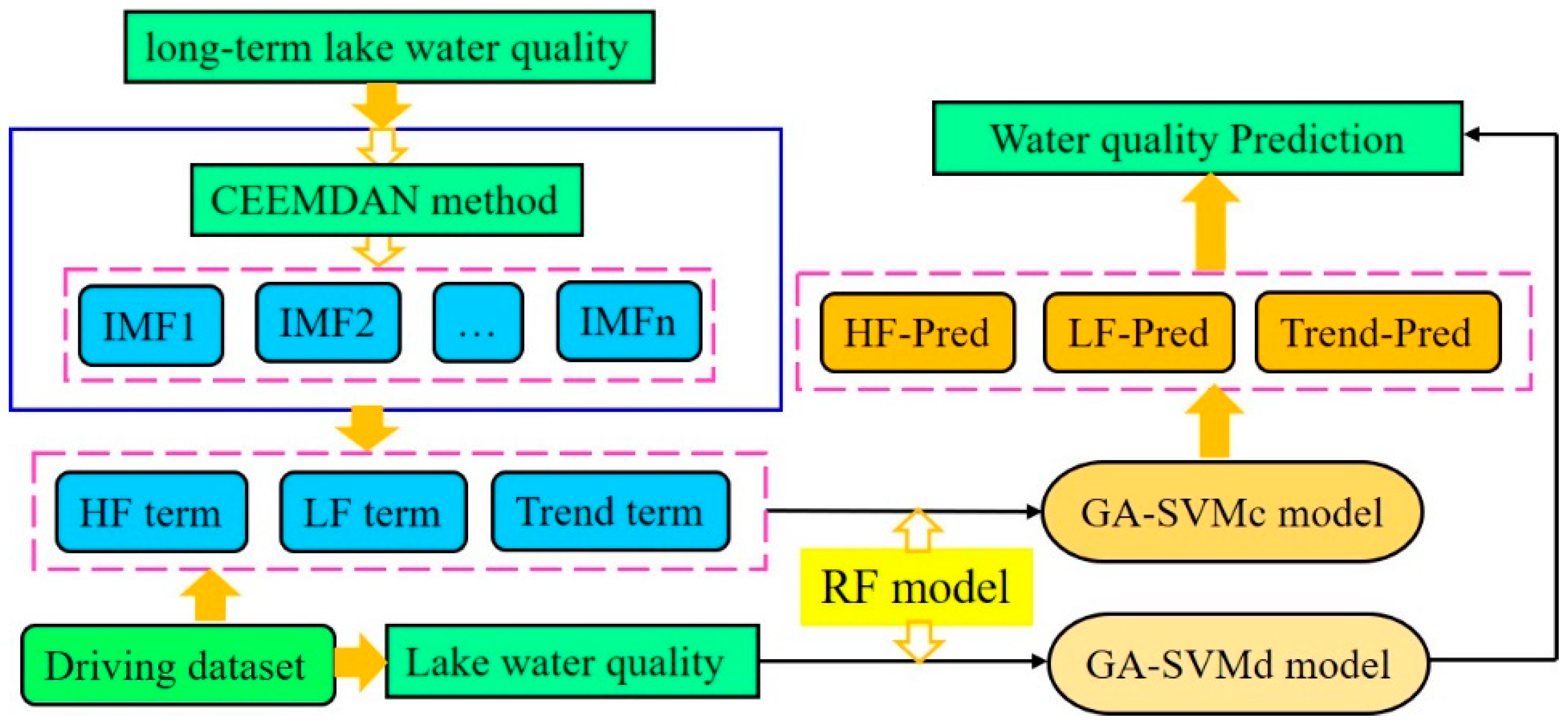
In this study, we integrated a framework that realized the decomposition-reclassification-driving factors identification-prediction for the water quality series. We decomposed the water quality sequences and reclassified them to evaluate the inner dynamic of water quality. Additionally, the water quality and the reclassified terms were set as the inputs for the GA-SVM model. We designed and examined two types of GA-SVM models based on the selected 10 driving factors for each corresponding term (the water quality term, the high-frequency term, the low-frequency term, and the trend term). We named the data-driven GA-SVM model for water quality the GA-SVMd model. More importantly, we used the RF method to identify the corresponding important driving factors for the high-frequency term, the low-frequency term, and the trend term. Then, the GA-SVM model was used to predict each term sequence. Finally, the water quality was obtained by the sum of each predicted term sequence. Thus, this model was defined as the GA-SVMc model (Figure 1).
3. Case Study of Beihu Lake, Wuhan City, China
3.1. Study Area
The Beihu catchment is situated on the eastern expansion edge of the Wuhan City and includes the majority of heavy industrial parks (Figure 2). As a result, the Beihu catchment has a relatively lagging underground pipe network and sewage treatment capacity. Furthermore, sewage water sources, such as industrial, domestic, runoff, and agricultural sources, contribute vastly without reasonable water treatment, and discharge directly in the surface water body. Thus, the multiple sources of sewage have caused the downstream water body of Beihu Lake to be heavily polluted for a long time. Recently, many countermeasures have been performed to control water pollution; however, significant improvement in water quality has not been observed [42].
The Beihu Lake is a semi-natural lake regulated by a pumping station. Furthermore, the Beihu Lake catchment is situated in the rural-urban marginal area. As a result, the complex LULC, urban stormwater network, and multi-source water pollution create a complex urban water system. In the wet season, the high frequency of rainfall events causes a large amount of runoff; moreover, the water level of the outer river is higher than the water table of the Beihu Lake. Therefore, pumping stations are needed to drain the lake water to the outer river. In the dry season, the runoff of the Beihu Lake is quite small, and the water table of the outer river is lower than the water table of the Beihu Lake; therefore, the water of the lake is free to discharge to the outer river. Consequently, the water table of the Beihu Lake level is a key factor, since it is a significant indicator of whether the pumping station needs to drain water from the lake and whether the lake can be discharged into the outer river via free flow. Evapotranspiration (ET) is also a key factor since the lake is an open water body with a large surface.
3.2. Water Quality and Other Monitored Datasets
In this study, the monthly water quality series from 15 January 2014 to 15 November 2021 were collected partly form environmental measurements by water samples and partly from Wuhan Ecological Environment Bureau [43], and the modeling period was set to the same period as the monitoring period. According to the monitored results, NH3-N and TN were confirmed to be the main pollutants in the study area (Table 1); therefore, NH3-N and TN were selected as the main water quality variables in this study. The hourly rainfall data and the water table of the Beihu lake were also monitored. Furthermore, the sums of 5-day, 10-day, 15-day, 20-day, monthly, seasonal, and yearly rainfall were calculated based on the hourly rainfall data. The 5-day, 10-day, 15-day, 20-days, and monthly average water table and accumulated variations of the water table were also calculated based on the hourly water table of the Beihu lake.
3.3. Remote Sensing-Based Data
Remote sensing-based data have significant contributions to the prediction of long-term water quality. In this study, three types of remote sensing data were used: land use and land cover, the ET dataset, and the nighttime light dataset (NTL) (Table 2). In detail, three periods of the Chinese Gaofen (GF)-1 data (resolution of 2 m) were manually identified to obtain the land use and land cover land metrics dataset for the years of 2014, 2017, 2020. The 8-day ET dataset [44], which ranges from 15 June 2015 to 15 November 2021, was downloaded from the MODIS Land Products (Net Evapotranspiration 8-Day L4 Global 500 m) (https://ladsweb.modaps.eosdis.nasa.gov/search/, accessed on 15 December 2021). Then, the monthly potential ET data were obtained by summing the total potential ET data on the 8-day total ET dataset for four periods of every month. Domestic wastewater discharge is a critical point pollutant source to the lake water quality; therefore, accurately evaluating the population has a significant effect on predicting water quality. The NTL dataset has been proven to be an effective dataset to obtain population data [45]. In this study, the yearly Visible Infrared Imaging Radiometer Suite (VIIRS) Day/Night Band (DNB) dataset was chosen to calculate the population [46].
The yearly VIIRS data were first corrected based on the assumption that the NTL value of the previous year is smaller than that of the next year (Equation (8)) [46].
Literature has proven that the NPP-VIIR NTL data can obtain a reasonable estimation of distributed population [46]. The correlation between NPP-VIIR NTL radiance and population follows Equation (9).
The precision of the calculated population and the real population was evaluated by Equation (10). If the calculated population had a relatively large error, the power function was then used to recorrect the calculated population until it obtained a reasonable result (Equation (11)).
where γ indicates the relative error. POPc and POPs indicate the calculated population by the NTL and statistical population. cn and fn indicate the correction and the adjusted DBN. POPn and POPtotal represent the nth yearly statistical population and the total statistical population during the calculated period.
4. Results
4.1. The Main Input Data from the Remote Sensing Dataset
4.1.1. Land Use and Land Cover (LULC), Land Metrics
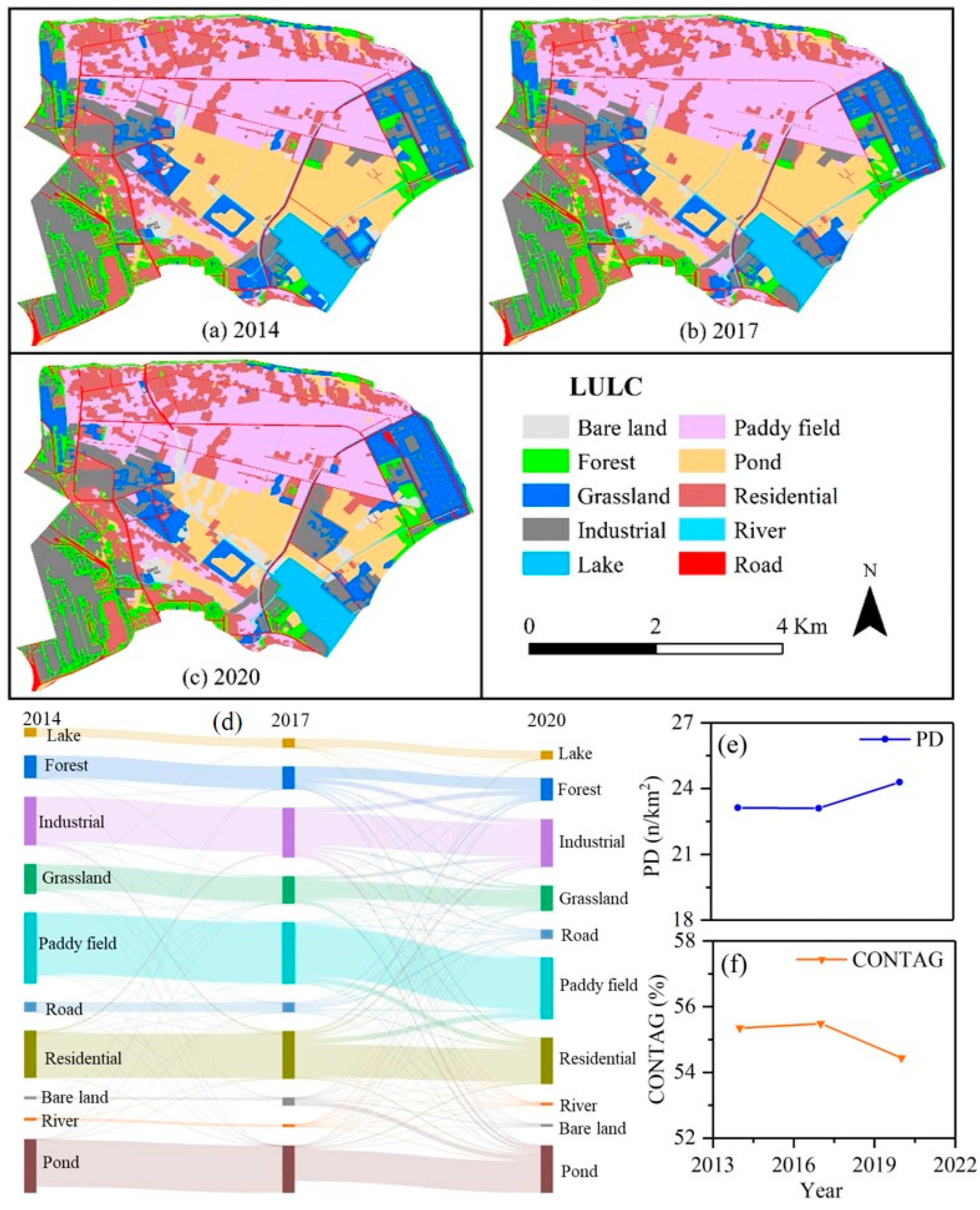
LULC has a remarkable influence on urban water system quality due to different rainfall-runoff response mechanisms and non-point sources pollution generation mechanisms. Especially in urban-rural marginal areas, land use types are significantly altered, changing the effective water amounts, nutrient levels, and surface roughness of the land surface directly, and thus changing the urban hydrological processes and ecological environments. In this study, the years 2014, 2017, 2020 were interpreted for water quality prediction. Results revealed that 11 types of LULC mainly existed in the Beihu catchment, i.e., lake, rivers, roads, grassland, forest land, ponds, paddy fields, bare land, industrial land, and residential land (Figure 3). The area of the ponds and paddy fields slightly declined during the study period, while the area of the industrial land and residential land increased due to the expansion of the urban area (Figure 3a–d). The area of forest/grassland also had a substantial influence on non-point sources, and was chosen as a driving factor in this study. The chosen land metrics were the patch density (PD) and contagion index (CONTAG) due to the high Person’s correlations of the other factors, such as the landscape shape index (LSI) and the largest patch index (LPI).
4.1.2. ET and POP Dataset
The average potential ET of the Beihu catchment exhibited strong seasonal variation (Figure 4a). The population calculated by the NPP-VIIR NTL radiance of Wuhan City performed well. The population of the Beihu catchment tended to decrease slowly in the early period and increase rapidly in the later period (Figure 4b). This might be due to the Beihu catchment being located at the edge of the urban area; people tended to migrate to the urban area in the early period, while when the urban gradually expanded, more areas of the catchment became urban areas; therefore, the population showed a trend of rapid growth in the later period. This result was consistent with the statistical data of Qingshan District, Wuhan City [47].
4.2. Decomposition and Reclassification of the Water Quality Series
All water quality sequences, i.e., the NH3-N and TN monitoring data from 15 January 2014 to 15 November 2021, were decomposed by the CEEMDAN method (Figure 5). Then, the decomposed IMFs terms and trend terms were reclassified based on the t-test (Figure 6).
The decomposed IMFs and the residue term by the CEEMDAN for NH3-N and TN are shown in Figure 5. In this study, 500 trials were implemented and the white noise coefficient was given as 0.2. Results revealed that both NH3-N and TN had four IMFs. From the high-frequency IMF to low-frequency IMF, the frequencies and amplitudes changed significantly and the amplitudes became smaller (Figure 5). The amplitudes of NH3-N and TN were 3 for IMF1 and then declined to 1.5–2 for IMF2-IMF3, while the amplitudes increased to 3 for IMF4 for NH3-N and TN. The residue term for NH3-N and TN increased and had relatively small amplitudes (Figure 5).
The mean period [39], mean values, the variance of each IMF, the percentage of the variance of the IMFs, and the Pearson correlation between each IMF with the water quality series were analyzed in this study (Table 3). Results revealed that IMF1 and IMF2 had more frequent fluctuations and had different mean periods for NH3-N and TN, while IMF3 and IMF4 had larger and similar mean periods (Table 3). The percentage of the variance of the IMFs confirmed that the IMF1 and IMF4 had the greatest proportion of contribution on the water quality.
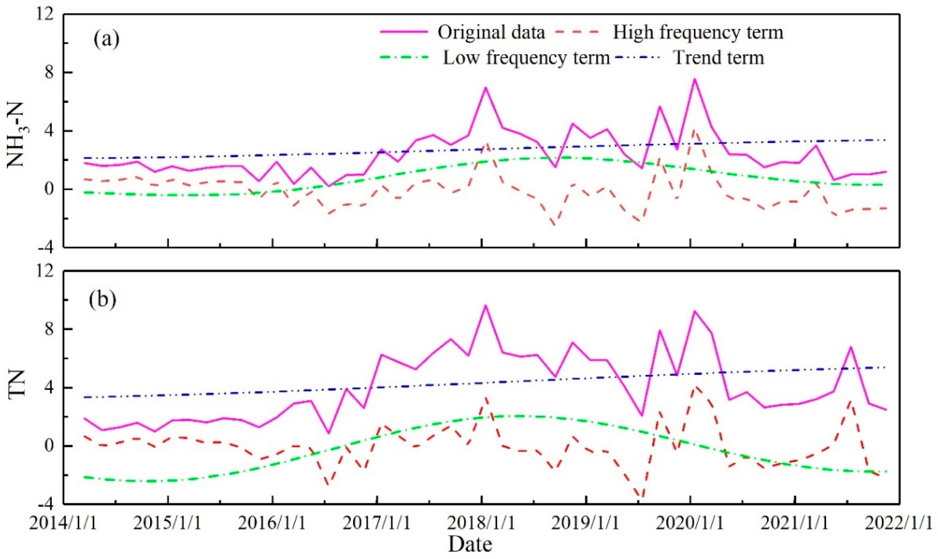
We reclassified the decomposed water quality of IMF1 to IMF4 and residual term based on the t-test in this study. The residual term was set as the trend term, IMF1 to IMF3 were reclassified as the high-frequency term for both NH3-N and TN due to the significant difference among the IMFs, and for IMF4, both NH3-N and TN were reclassified as the low-frequency term. The original water quality series and the reclassified high-frequency, low-frequency, and trend term are shown in Figure 6. Results confirmed that the high-frequency terms for both NH3-N and TN had stronger fluctuation frequencies, which were similar to the water quality series. The low-frequency terms for both NH3-N and TN showed a tendency of first increasing and then decreasing, and the trend of the low-frequency terms was similar to the water quality trend. The trend terms for NH3-N and TN increased in the whole monitoring period and gradually leveled at the end of the monitoring period.
4.3. Evaluation of the Importance of Driving Factors
We used the RF method to estimate the importance of driving factors (determined by the relative importance for all driving factors), which was used for both the GA-SVMd model and the GA-SVMc model. As shown in Figure 7, the relative importance of driving factors significantly varied between the water quality variables and the corresponding data series and different frequencies.
Regarding the NH3-N of the Beihu Lake for the GA-SVMd model, the main driving factors were hydro-meteorological factors, i.e., ET, seasonal rainfall, the cumulative magnitude of change in the lake water table over 10 days, the average lake water table over 10 days, and the sum rainfall over 20 days. Furthermore, population, pond land, and forest/grassland were also relatively important influences. When analyzing the importance of the driving factors on the decomposed and reclassified results of the CEEMDAN, the driving factors of the high-frequency term for NH3-N were dominated by the hydrometeorological factors; only the population had a slight effect. The driving factors on the low-frequency term for NH3-N were dominated by yearly rainfall, the population, LUCC (such as the pond, the forest/grassland, and the paddy field), and land metrics (the PD, the CONTAG). The different days of the cumulative magnitude lake water table also had a relatively significant impact on NH3-N. In detail, field investigation confirmed that the industrial point sources were the main source of NH3-N; therefore, the industrial land area had the most significant effect on the trend term of NH3-N. The impervious surface, the paddy field, the population, and the cumulative magnitude of change in the lake water table over 5, 20, and 10 days were also the main driving factors for the trend term of NH3-N.
Compared to the GA-SVMd model, the driving factors for TN also included many hydro-meteorological factors, i.e., the ET, the yearly rainfall, the sum rainfall over 5 days, and the average lake water table over 30 days. Moreover, paddy field land, impervious surface (defined as the sum of the residential, industrial, and road land), population, and PD also had significant influence on TN (Figure 7). When analyzing the importance of the driving factors on the decomposed and reclassified results of the CEEMDAN, the driving factors also significantly varied from the high-frequency term to trend terms for TN. The driving factors of the high-frequency term for TN were dominated by the hydrometeorological factors; only the population had a slight effect. The driving factors on the low-frequency term for TN were also dominated by yearly rainfall, population, LUCC, and land metrics. The driving factors on the trend term for TN were mainly influenced by the population, the LUCC, land metrics, and yearly rainfall. Residential recharge was proven to be the main source of TN by previous studies (Hwang et al., 2016; Paule et al., 2014), which is related to the most important driving factor (the population) for the trend term of TN (Figure 7).
4.4. Prediction of Water Quality by the GA-SVMd Model and the GA-SVMc Model
The proportion of the calibration period and the validation period was set as 0.7 for both NH3-N and TN; i.e., the period from 1 July 2015 to 15 January 2020 was set as the calibration period, and the period from 15 January 2015 to 15 November 2021 was set as the validation period. The results modeling with the GA-SVMd model and the GA-SVMc model both showed reasonable performance (Figure 8, Table 4). Apparently, the GA-SVMc model performed better in the prediction of water quality. Furthermore, the GA-SVMc model provided more accurate prediction results on the strong variations of water quality. However, the simulation accuracy of GA-SVMd model and the GA-SVMc were poor when the water quality dramatically changed, which may be due to the lack of measured runoff data in the study area. Non-point source pollution was usually the main pollution source during the rainfall-runoff process [48]. Therefore, it is necessary to strengthen the monitoring of runoff and water quality during rainfall in future research.
5. Discussion
5.1. Important Factors Dominating Water Pollution and Different Frequency Terms of Water Quality
The water pollution of urban-rural marginal areas is attributed to many factors, such as LULC, land metrics, hydro-meteorological factors, and point sources recharged by the domestic and industrial [4,33,49]. Land surface runoff is usually set as an essential factor for predicting water quality in data-driven models [33]. The runoff was significantly complex due to the multiple inputs and has not been monitored over a long time series. In this study, the lake water table was affected by the recharge of rainfall-runoff sources, domestic sources and industrial sources; controlled by the pumping gate, it could be set as a substitute factor for runoff to predict water quality and obtain reasonable performance. The factors of the LULC and land metrics for the urban-rural marginal area changed significantly due to the rapid expansion of the urban area, and thus had notable impacts on water quality, as has confirmed by many studies [50,51,52]. In this study, results confirmed that LULC and land metrics had a relatively high impact on the low-frequency and trend term of water quality. Point sources, such as industrial wastewater discharge and domestic wastewater discharge, also had significant impacts on water quality [12]. Our results confirmed that the population was the dominant pollution source of TN, and also had a relative effect on NH3-N. Industrial land had a significant impact on NH3-N and a similar effect on TN. Meteorological conditions, such as rainfall and the ET, also had significant and complex impacts on water quality [51]. For example, the first rainfall was confirmed to have a significant impact on water quality in the urban area, while seasonal rainfall had a greater effect on agricultural land water quality [53,54]. Our results also confirmed that rainfall and the ET had significant effects on water quality, and dominated the high-frequency term of water quality.
5.2. Prediction of the Urban Water Quality by Machine Learning Models
Considering the strongly changing LULC, the complexity of diverse and continuous varied pollution sources and hydro-hydraulic conditions, meteorological conditions with complex dynamic characteristics, and the widespread lack of data in rural-urban marginal areas, developing a prediction model with reasonable performance is still a tremendous challenge [4,33,35,55]. The original data-driven machine learning models seemed to provide a good choice to simulate the urban-rural catchment water quality with complex and data-lacking conditions [33]. In a fact, point sources, such as industrial discharge, have not been well monitored for a long time. Runoff volumes have also not been monitored and the complexity could not easily be modeled. However, the original data-driven machine learning models, i.e., the GA-SVDd model in our study, still performed reasonably due to the substantial data obtained from the remote sensing data and the lake water table (Figure 8).
A successful model could both be used to reveal the inner dynamics and driving mechanisms and provide accurate prediction results. Previous studies have integrated many models to reveal the inner features of the time series data, such as runoff and water quality. The EMD method, the EEMD method, the CEEMDAN method, and the WT method have been widely used to decompose time series data, after which they integrated with machine learning models [25,28,36]. However, not all the integrated models achieve better prediction performance; Zhang et al. [36] confirmed that EMD-based integrated models may perform worse than data-driven models in simulating streamflow. In our study, prediction results from the integrated GA-SVMc model confirmed that the CEEMDAN integrated with the GA-SVM model for water quality can achieve markedly better performance than the original SVM model.
6. Conclusions
Evaluation of the dynamic and influence mechanisms, and the prediction of variations of water quality provide early warning and guidance to reduce water pollution concentration. The limited monitoring data and the complexity of the water system restrict the prediction of long-term water quality. However, the multiple variables derived from remote-sensing data (ET, LULC, etc.) provide scientific data and reasonably reveal the variation mechanism.
In this study, we developed an integrated decomposition-reclassification-prediction method for water quality by integrating the CEEMDAN method, the RF method, and a genetic algorithm-support vector machine model (GA-SVM). The degression of the long-term water quality was decomposed and reclassified into three different frequency terms, i.e., the high-frequency, low-frequency, and trend terms, to reveal the inner mechanisms and dynamics in the CEEMDAN method. The RF method was then used to identify the teleconnection and the significance of the selected driving factors. More importantly, the GA-SVM model was integrated and designed in two types of model schemes, which were the data-driven model (GA-SVMd) and the integrated CEEMDAN-GA-SVM model (defined as GA-SVMc model), in order to predict urban water quality. Results revealed that the high-frequency terms for NH3-N and TN had a major contribution to the water quality and were mainly dominated by the hydrometeorological factors, such as the ET, rainfall, and dynamics of the lake water table. The low-frequency terms for NH3-N and TN were both dominated by yearly rainfall, population, LULC, and land metrics. The trend terms revealed that the water quality continuously deteriorated during the study period and was mainly regulated by the LULC and land metrics factor, population, and yearly rainfall. The prediction results confirmed that the integrated GA-SVMc model achieved better performance than a single data-driven model such as GA-SVM.
Author Contributions
Conceptualization, Z.Y. and L.Z.; methodology, Z.Y. and L.Z.; software, Z.Y.; validation, Z.Y., L.Z. and D.C.; formal analysis, Z.Y., L.Z. and J.X.; investigation, Z.Y. and L.Z.; resources, L.Z.; data curation, L.Z. and Y.Q.; writing—original draft preparation, Z.Y.; writing—review and editing, L.Z.; visualization, Z.Y. and L.Z.; supervision, L.Z.; funding acquisition, J.X. and L.Z.; Data curation, D.C.; Investigation, D.C. All authors have read and agreed to the published version of the manuscript.
Funding
This research was funded by the Strategic Priority Research Program of the Chinese Academy of Sciences (Grant No. XDA23040304) and the National Nature Science Foundation of China (No. 41890823).
Data Availability Statement
Not applicable.
Acknowledgments
We thank the anonymous reviewers for their constructive feedback.
Conflicts of Interest
The authors declare no conflict of interest.
References
- Cheng, F.Y.; Basu, N.B. Biogeochemical hotspots: Role of small water bodies in landscape nutrient processing. Water Resour. Res. 2017, 53, 5038–5056. [Google Scholar] [CrossRef] [Green Version]
- Freni, G.; Mannina, G.; Viviani, G. Assessment of the integrated urban water quality model complexity through identifiability analysis. Water Res. 2011, 45, 37–50. [Google Scholar] [CrossRef] [PubMed]
- Forman, R.; Wu, J. Where to put the next billion people. Nature 2016, 537, 608–611. [Google Scholar] [CrossRef]
- Carey, R.O.; Migliaccio, K.W.; Li, Y.; Schaffer, B.; Kiker, G.A.; Brown, M.T. Land use disturbance indicators and water quality variability in the Biscayne Bay Watershed, Florida. Ecol. Indic. 2011, 11, 1093–1104. [Google Scholar] [CrossRef]
- Mello, K.; de Valente, R.A.; Randhir, T.O.; dos Santos, A.C.A.; Vettorazzi, C.A. Effects of land use and land cover on water quality of low-order streams in Southeastern Brazil: Watershed versus riparian zone. Catena 2018, 167, 130–138. [Google Scholar] [CrossRef]
- Pan, D.; Hong, W.; Kong, F. Efficiency evaluation of urban wastewater treatment: Evidence from 113 cities in the Yangtze River Economic Belt of China. J. Environ. Manag. 2020, 270, 110940. [Google Scholar] [CrossRef] [PubMed]
- Jia, X.; O’Connor, D.; Hou, D.; Jin, Y.; Li, G.; Zheng, C.; Ok, Y.S.; Tsang, D.S.W.; Luo, J. Groundwater depletion and contamination: Spatial distribution of groundwater resources sustainability in China. Sci. Total Environ. 2019, 672, 551–562. [Google Scholar] [CrossRef]
- Dunalska, J.A.; Grochowska, J.; Wiśniewski, G.; Napiórkowska-Krzebietke, A. Can we restore badly degraded urban lakes? Ecol. Eng. 2015, 82, 432–441. [Google Scholar] [CrossRef]
- Freni, G.; Mannina, G. Uncertainty in water quality modelling: The applicability of Variance Decomposition Approach. J. Hydrol. 2010, 394, 324–333. [Google Scholar] [CrossRef]
- Schellart, A.N.A.; Tait, S.J.; Ashley, R.M. Towards quantification of uncertainty in predicting water quality failures in integrated catchment model studies. Water Res. 2010, 44, 3893–3904. [Google Scholar] [CrossRef]
- Dhakal, K.P.; Chevalier, L.R. Urban Stormwater Governance: The Need for a Paradigm Shift. Environ. Manag. 2016, 57, 1112–1124. [Google Scholar] [CrossRef] [PubMed]
- Garnier, J.; Brion, N.; Callens, J.; Passy, P.; Deligne, C.; Billen, G.; Servais, P.; Billen, C. Modeling historical changes in nutrient delivery and water quality of the Zenne River (1790s–2010): The role of land use, waterscape and urban wastewater management. J. Mar. Syst. 2013, 128, 62–76. [Google Scholar] [CrossRef]
- Tong, S.; Li, X.; Zhang, J.; Bao, Y.; Bao, Y.; Na, L.; Si, A. Spatial and temporal variability in extreme temperature and precipitation events in Inner Mongolia (China) during 1960–2017. Sci. Total Environ. 2018, 649, 75–89. [Google Scholar] [CrossRef] [PubMed]
- Ali, R.; Kuriqi, A.; Abubaker, S.; Kisi, O. Long-Term Trends and Seasonality Detection of the Observed Flow in Yangtze River Using Mann-Kendall and Sen’s Innovative Trend Method. Water 2019, 11, 1855. [Google Scholar] [CrossRef] [Green Version]
- Yenilmez, F.; Keskin, F.; Aksoy, A. Water quality trend analysis in Eymir Lake, Ankara. Phys. Chem. Earth Parts A/B/C 2011, 36, 135–140. [Google Scholar] [CrossRef]
- Huang, N.E.; Wu, Z. A review on Hilbert-Huang transform: Method and its applications to geophysical studies. Rev. Geophys. 2008, 46, 228–251. [Google Scholar] [CrossRef] [Green Version]
- Chou, C.-M. Wavelet-Based Multi-Scale Entropy Analysis of Complex Rainfall Time Series. Entropy 2011, 13, 241–253. [Google Scholar] [CrossRef] [Green Version]
- Liu, H.-L.; Bao, A.-M.; Chen, X.; Wang, L.; Pan, X. Response analysis of rainfall-runoff processes using wavelet transform: A case study of the alpine meadow belt. Hydrol. Process. 2011, 25, 2179–2187. [Google Scholar] [CrossRef]
- Ruiming, F. Wavelet based relevance vector machine model for monthly runoff prediction. Water Qual. Res. J. 2018, 54, 134–141. [Google Scholar] [CrossRef]
- Kang, S.; Lin, H. Wavelet analysis of hydrological and water quality signals in an agricultural watershed. J. Hydrol. 2007, 338, 1–14. [Google Scholar] [CrossRef]
- Niu, M.; Wang, Y.; Sun, S.; Li, Y. A novel hybrid decomposition-and-ensemble model based on CEEMD and GWO for short-term PM2.5 concentration forecasting. Atmos. Environ. 2016, 134, 168–180. [Google Scholar] [CrossRef]
- Huang, N.E.; Shen, Z.; Long, S.R. The empirical mode decomposition and the Hilbert spectrum for nonlinear and nonstationary time series analysis. Proc. R. Soc. Lond. 1998, 454, 903–995. [Google Scholar] [CrossRef]
- Xiao, X.; He, J.; Yu, Y.; Cazelles, B.; Li, M.; Jiang, Q.; Xu, C. Teleconnection between phytoplankton dynamics in north temperate lakes and global climatic oscillation by time-frequency analysis. Water Res. 2019, 154, 267–276. [Google Scholar] [CrossRef] [PubMed]
- Ouyang, Q.; Lu, W.; Xin, X.; Zhang, Y.; Cheng, W.; Yu, T. Monthly Rainfall Forecasting Using EEMD-SVR Based on Phase-Space Reconstruction. Water Resour. Manag. 2016, 30, 2311–2325. [Google Scholar] [CrossRef]
- Yuan, R.; Cai, S.; Liao, W.; Lei, X.; Zhang, Y.; Yin, Z.; Dingm, G.; Wang, J.; Xu, Y. Daily Runoff Forecasting Using Ensemble Empirical Mode Decomposition and Long Short-Term Memory. Front. Earth Sci. 2021, 9, 621780. [Google Scholar] [CrossRef]
- Fijani, E.; Barzegar, R.; Deo, R.; Tziritis, E.; Konstantinos, S. Design and implementation of a hybrid model based on two-layer decomposition method coupled with extreme learning machines to support real-time environmental monitoring of water quality parameters. Sci. Total Environ. 2018, 154, 267–276. [Google Scholar] [CrossRef]
- Huan, J.; Cao, W.; Qin, Y. Prediction of dissolved oxygen in aquaculture based on EEMD and LSSVM optimized by the Bayesian evidence framework. Comput. Electron. Agric. 2018, 150, 257–265. [Google Scholar] [CrossRef]
- Zhang, J.; Tang, H.; Tannant, D.D.; Lin, C.; Xia, D.; Liu, X.; Zhang, Y.; Ma, J. Combined forecasting model with CEEMD-LCSS reconstruction and the ABC-SVR method for landslide displacement prediction. J. Clean. Prod. 2021, 293, 126205. [Google Scholar] [CrossRef]
- Joshi, P.; Leitão, J.P.; Maurer, M.; Bach, P.M. Not all SuDS are created equal: Impact of different approaches on combined sewer overflows. Water Res. 2021, 191, 116780. [Google Scholar] [CrossRef] [PubMed]
- Van Daal-Rombouts, P.; Sun, S.; Langeveld, J.; Bertrand-Krajewski, J.-L.; Clemens, F. Design and performance evaluation of a simplified dynamic model for combined sewer overflows in pumped sewer systems. J. Hydrol. 2016, 538, 609–624. [Google Scholar] [CrossRef] [Green Version]
- Coutu, S.; Del Giudice, D.; Rossi, L.; Barry, D.A. Parsimonious hydrological modeling of urban sewer and river catchments. J. Hydrol. 2012, 464–465, 477–484. [Google Scholar] [CrossRef] [Green Version]
- Tan, K.M.; Seow, W.K.; Wang, C.L.; Kew, H.J.; Parasuraman, S.B. Evaluation of performance of Active, Beautiful and Clean (ABC) on stormwater runoff management using MIKE URBAN: A case study in a residential estate in Singapore. Urban Water J. 2019, 16, 156–162. [Google Scholar] [CrossRef]
- Zhi, W.; Feng, D.; Tsai, W.-P.; Sterle, G.; Harpold, A.; Shen, C.; Li, L. From Hydrometeorology to River Water Quality: Can a Deep Learning Model Predict Dissolved Oxygen at the Continental Scale? Environ. Sci. Technol. 2021, 55, 2357–2368. [Google Scholar] [CrossRef]
- Qiao, Z.; Sun, S.; Jiang, Q.; Xiao, L.; Wang, Y.; Yan, H. Retrieval of Total Phosphorus Concentration in the SurfaceWater of Miyun Reservoir Based on Remote Sensing Data and Machine Learning Algorithms. Remote Sens. 2021, 13, 4662. [Google Scholar] [CrossRef]
- Mohammadpour, R.; Shaharuddin, S.; Chang, C.K.; Zakaria, N.A.; Ghani, A.A.; Chan, N.W. Prediction of water quality index in constructed wetlands using support vector machine. Environ. Sci. Pollut. Res. 2014, 22, 6208–6219. [Google Scholar] [CrossRef] [PubMed]
- Zhang, X.; Peng, Y.; Zhang, C.; Wang, B. Are hybrid models integrated with data preprocessing techniques suitable for monthly streamflow forecasting? Some experiment evidences. J. Hydrol. 2015, 530, 137–152. [Google Scholar] [CrossRef]
- Wu, Z.; Huang, N.E. Ensemble empirical mode decomposition: A noiseassisted data analysis method. Adv. Adapt. Data Anal. 2009, 1, 1–41. [Google Scholar] [CrossRef]
- Yeh, J.R.; Shieh, J.S.; Huang, N.E. Complementary ensemble empirical mode decomposition: A novel noise enhanced data analysis method. Adv. Adapt. Data Anal. 2010, 2, 135–156. [Google Scholar] [CrossRef]
- Zhang, X.; Lai, K.K.; Wang, S.-Y. A new approach for crude oil price analysis based on Empirical Mode Decomposition. Energy Econ. 2008, 30, 905–918. [Google Scholar] [CrossRef]
- Wu, C.; Fang, C.; Wu, X.; Zhu, G. Health-Risk Assessment of Arsenic and Groundwater Quality Classification Using Random Forest in the Yanchi Region of Northwest China. Expo. Health 2020, 12, 761–774. [Google Scholar] [CrossRef]
- Marler, R.; Arora, J. Survey of multi-objective optimization methods for engineering. Struct. Multidiscip. Optim. 2004, 26, 369–395. [Google Scholar] [CrossRef]
- Wuhan Ecological Environment Bureau. Report of Water Quality of Centralized Drinking Water Sources in Urban and County Level of Wuhan City. 2021. Available online: http://hbj.wuhan.gov.cn/hjsj/ (accessed on 15 December 2021). (In Chinese)
- Wuhan Ecological Environment Bureau. Hubei Province Pollution Source Environmental Information Release System. 2021. Available online: http://113.57.151.5:4504/EAFMS/Guest.aspx (accessed on 15 December 2021). (In Chinese)
- Mu, Q.; Zhao, M.; Running, S.W. Improvements to a MODIS global terrestrial evapotranspiration algorithm. Remote Sens. Environ. 2011, 115, 1781–1800. [Google Scholar] [CrossRef]
- Yu, M.; Guo, S.; Guan, Y.; Cai, D.; Zhang, C.; Fraedrich, K.; Liao, Z.; Zhang, X.; Tian, Z. Spatiotemporal Heterogeneity Analysis of Yangtze River Delta Urban Agglomeration: Evidence from Nighttime Light Data (2001–2019). Remote Sens. 2021, 13, 1235. [Google Scholar] [CrossRef]
- Elvidge, C.D.; Baugh, K.; Zhizhin, M.; Hsu, F.C.; Ghosh, T. VIIRS night-time lights. Int. J. Remote Sens. 2017, 38, 5860–5879. [Google Scholar] [CrossRef]
- Wuhan Municipal Bureau of Statistics; NBS Survey Office in Wuhan. Wuhan Statistical Yearbook; China Statistics Press Co., Ltd.: Wuhan, China, 2021. Available online: http://tjj.hubei.gov.cn/tjsj/sjkscx/tjnj/gsztj/whs/202201/P020220125601159778648.pdf (accessed on 15 January 2022). (In Chinese)
- Huang, F.; Wang, X.; Lou, L.; Zhou, Z.; Wu, J. Spatial variation and source apportionment of water pollution in Qiantang River (China) using statistical techniques. Water Res. 2010, 44, 1562–1572. [Google Scholar] [CrossRef] [PubMed]
- Seeboonruang, U. A statistical assessment of the impact of land uses on surface water quality indexes. J. Environ. Manag. 2012, 101, 134–142. [Google Scholar] [CrossRef] [PubMed]
- Yang, K.; Luo, Y.; Chen, K.; Yang, Y.; Shang, C.; Yu, Z.; Xu, J.; Zhao, Y. Spatial–Temporal variations in urbanization in Kunming and their impact on urban lake water quality. Land Degrad. Dev. 2020, 31, 1392–1407. [Google Scholar] [CrossRef]
- Mello, K.; de Taniwaki, R.H.; Paula FR de Valente, R.A.; Randhir, T.O.; Macedo, D.R.; Leal, C.G.; Rodrigues, C.B.; Hughes, R.M. Multiscale land use impacts on water quality: Assessment, planning, and future perspectives in Brazil. J. Environ. Manag. 2020, 270, 110879. [Google Scholar] [CrossRef] [PubMed]
- Zhang, J.; Li, S.; Jiang, C. Effects of land use on water quality in a River Basin (Daning) of the Three Gorges Reservoir Area, China: Watershed versus riparian zone. Ecol. Indic. 2020, 113, 106226. [Google Scholar] [CrossRef]
- Lewis, W.M. Physical and Chemical Features of Tropical Flowing Waters. Trop. Stream Ecol. 2008, 1–21. [Google Scholar] [CrossRef]
- Shi, P.; Zhang, Y.; Li, Z.; Li, P.; Xu, G. Influence of land use and land cover patterns on seasonal water quality at multi-spatial scales. Catena 2017, 151, 182–190. [Google Scholar] [CrossRef]
- Jia, Q.M.; Li, Y.P.; Liu, Y.R. Modeling urban eco-environmental sustainability under uncertainty: Interval double-sided chance-constrained programming with spatial analysis. Ecol. Indic. 2020, 115, 106438. [Google Scholar] [CrossRef]
Figure 1.
The two designed integrated experimental schemes. HF term and LF term represent the high-frequency and low-frequency terms. HF-Pre, LF-Pre, and Trend-Pre indicate the prediction of the high-frequency, low-frequency, and trend terms.
Figure 1.
The two designed integrated experimental schemes. HF term and LF term represent the high-frequency and low-frequency terms. HF-Pre, LF-Pre, and Trend-Pre indicate the prediction of the high-frequency, low-frequency, and trend terms.

Figure 2.
The study area of the Beihu catchment.

Figure 3.
Land use and land change (a–d); land metrics (e,f).

Figure 4.
The potential monthly ET (a); the yearly population of the Beihu catchment (b).

Figure 5.
The decomposition of water quality sequences by the CEEMDAN method. (a) NH3-N; (b) TN.

Figure 6.
The reclassified terms and the original water quality series. (a) NH3-N; (b) TN.

Figure 7.
The relative importance of the driving factors. The R5DS, R10DS, R20DS, RS, and RY represent the sum rainfall over 5 days, 10 days, 20 days, seasonally, and yearly. The WT5DAc, WT10DAc, WT15DAc, WT20DAc, and WT30DAc indicate the cumulative magnitude of change in the lake water table over 5 days, 10 days, 15 days, 20 days, and 30 days. The WT5Av, WT10Av, WT15Av, WT20Av, and WT30Av indicate the average lake water table over 5 days, 10 days, 15 days, 20 days, and 30 days. FG represents forest/grassland. POP represents the population. IMPS indicates impervious surface.

Figure 8.
The prediction results of the GA-SVMd model and GA-SVMc model. (a) NH3-N; (b) TN.


Table 1.
Statistics of the water quality in the Beihu catchment.
| Water Quality Variable | Units | Mean | Standard Deviation |
|---|---|---|---|
| NH3-N | mg/L | 2.59 | 1.69 |
| TN | mg/L | 4.56 | 2.29 |
Table 2.
Statistics of the related data details.
| No. | Data | Unit | Temporal and Spatial Resolution | Data Sources |
|---|---|---|---|---|
| 1 | Rainfall | mm | 1 h | Field investigation |
| 2 | Lake water table | m | 1 h | |
| 3 | Annual District Population | people | 1 year | Statistical yearbook |
| 4 | Land use and land cover | m | 2 m | Chinese Gaofen (GF)-1 |
| 5 | ET | mm | 8 days, 500 m | https://ladsweb.modaps.eosdis.nasa.gov/search/, accessed on 15 December 2021 |
| 6 | Nighttime light | m | 1 year, 500 m | https://eogdata.mines.edu/products/vnl/, accessed on 15 December 2021 |
Table 3.
The IMFs and the residue values for the decomposed long-term water quality data.
| Variable | IMF1 | IMF2 | IMF3 | IMF4 | Residue | |
|---|---|---|---|---|---|---|
| Mean period (Month) | NH3-N | 1.31 | 2.94 | 7.83 | 23.5 | 47 |
| TN | 1.47 | 3.92 | 7.83 | 23.5 | 47 | |
| Mean | NH3-N | −0.054 | −0.030 | −0.024 | 0.796 | 2.742 |
| TN | −0.052 | 0.038 | −0.018 | −0.273 | 4.348 | |
| Variance | NH3-N | 0.83 | 0.52 | 0.65 | 0.89 | 0.41 |
| TN | 1.15 | 0.83 | 0.57 | 1.55 | 0.65 | |
| Variance as % of (ΣIMFs + residual) | NH3-N | 25.17 | 15.86 | 19.70 | 26.96 | 12.31 |
| TN | 24.15 | 17.56 | 12.08 | 32.57 | 13.64 | |
| Pearson correlation | NH3-N | 0.50 | 0.46 | 0.44 | 0.65 | 0.27 |
| TN | 0.46 | 0.32 | 0.28 | 0.74 | 0.42 |
Table 4.
The modeled accuracy results in the calibration period and the validation period.
| Water Quality Variables | Evaluation Function | Calibration Period | Validation Period | ||
|---|---|---|---|---|---|
| GA-SVMd | GA-SVMc | GA-SVMd | GA-SVMc | ||
| NH3-N | NSE | 0.63 | 0.81 | 0.51 | 0.62 |
| RMSE | 0.97 | 1.28 | 1.7 | 1.14 | |
| TN | NSE | 0.57 | 0.77 | 0.55 | 0.61 |
| RMSE | 1.46 | 1.07 | 1.57 | 1.48 | |
Publisher’s Note: MDPI stays neutral with regard to jurisdictional claims in published maps and institutional affiliations. |
© 2022 by the authors. Licensee MDPI, Basel, Switzerland. This article is an open access article distributed under the terms and conditions of the Creative Commons Attribution (CC BY) license (https://creativecommons.org/licenses/by/4.0/).
Share and Cite
MDPI and ACS Style
Yang, Z.; Zou, L.; Xia, J.; Qiao, Y.; Cai, D. Inner Dynamic Detection and Prediction of Water Quality Based on CEEMDAN and GA-SVM Models. Remote Sens. 2022, 14, 1714. https://doi.org/10.3390/rs14071714
AMA Style
Yang Z, Zou L, Xia J, Qiao Y, Cai D. Inner Dynamic Detection and Prediction of Water Quality Based on CEEMDAN and GA-SVM Models. Remote Sensing. 2022; 14(7):1714. https://doi.org/10.3390/rs14071714
Chicago/Turabian StyleYang, Zhizhou, Lei Zou, Jun Xia, Yunfeng Qiao, and Diwen Cai. 2022. "Inner Dynamic Detection and Prediction of Water Quality Based on CEEMDAN and GA-SVM Models" Remote Sensing 14, no. 7: 1714. https://doi.org/10.3390/rs14071714
Note that from the first issue of 2016, this journal uses article numbers instead of page numbers. See further details here.