
Detection of Tree Decline (Pinus pinaster Aiton) in European Forests Using Sentinel-2 Data


1
CITEUC, Department of Earth Sciences, University of Coimbra, 3030-790 Coimbra, Portugal
2
Centre for Functional Ecology, Department of Life Sciences, University of Coimbra, 3000-456 Coimbra, Portugal
*
Author to whom correspondence should be addressed.
Remote Sens. 2022, 14(9), 2028; https://doi.org/10.3390/rs14092028
Submission received: 7 March 2022
/
Revised: 18 April 2022
/
Accepted: 19 April 2022
/
Published: 23 April 2022
(This article belongs to the Special Issue Remote Sensing and Smart Forestry)
Abstract
:Moderate-resolution satellite imagery is essential to detect conifer tree decline on a regional scale and address the threat caused by pinewood nematode (PWN), (Bursaphelenchus xylophilus. This is a quarantine organism responsible for pine wilt disease (PWD), which has caused substantial ecological and economic losses in the maritime pine (Pinus pinaster) forests of Portugal. This study describes the first instance of a pre-operational algorithm applied to Sentinel-2 imagery to detect PWD-compatible decline in maritime pine. The Random Forest model relied on a pre-wilting and an in-season image, calibrated with data from a 24-month long field campaign enhanced with Worldview-3 data and the analysis of biological samples (hyperspectral reflectance, pigment quantification in needles, and PWN identification). Independent validation results attested to the good performance of the model with an overall accuracy of 95%, particularly when decline affects more than 30% of the 100 m2 pixel of Sentinel-2. Spectral angle mapper applied to hyperspectral measurements suggested that PWN infection cannot be separated from other drivers of decline in the visible-near infrared domain. Our algorithm can be employed to detect regional decline trends and inform subsequent aerial and field surveys, to further investigate decline hotspots.
1. Introduction
Multiple causal agents lead to temporary or irreversible tree decline in European temperate forests. Abiotic and biotic agents often act in synergy [1], disrupting ecosystems and value chains, thus creating both tangible and intangible losses to local communities [2]. Purposeful or accidental introduction of alien species, a common issue in a world of global trade, can also severely compromise the stability of ecosystems. This was the case in the years following the detection of the pinewood nematode (PWN), Bursaphelenchus xylophilus (Steiner and Bührer, 1934) Nickle, 1970 in Europe [3].
PWN is native to North America but it is now found in Asian and European countries [4], including Portugal (mainland) [3], Spain [5,6], and the Madeira Island [7]. Given the threat posed by this nematode to conifers, it is listed as a quarantine organism by the European and Mediterranean Plant Protection Organization [8]. Specific rules and regulations have also been adopted by national and international organisms to contain this biotic agent. These included several directives issued by the European Commission, designed to curb the spread of PWN beyond the borders of Portugal.
PWN is the causal agent of the pine wilt disease (PWD), which is spread by pine beetles mainly belonging to the genus Monochamus. In Portugal and Spain, the only Monochamus species known as a vector is M. galloprovincialis (Olivier) [9,10]. Even though several conifers are vulnerable to PWN infection, maritime pine (Pinus pinaster Aiton) is the most susceptible host tree in Portugal. This species was once the most abundant in the country, but recent estimates now rank it as the third most common species due to widespread wildfires and PWD [11].
PWN transmission can occur in two ways: (i) primary transmission through feeding wounds, in which nematodes carried by beetles move into the tree [4,12], and; (ii) secondary transmission, during oviposition under the bark of stressed trees [4,13]. PWN causes a decrease in photosynthesis, xylemic dysfunction, water transport blocking, and affects cortex anatomy. Ultimately, it leads to parenchyma cell senescence, cambium destruction and a quick death (within weeks to months) [14]. However, symptoms are non-specific and include a decrease in resin exudation, needle browning and wilting, and drying of the crown. From a management perspective, the earliest and most obvious symptom is the discoloration of needles, which sets in early in the decline process and is associated with a reduction of photosynthetic pigments [15].
Since the symptoms are non-specific, field surveys must be focused on monitoring conifer trees showing decline symptoms, particularly a totally or partially dried crown or an unusual coloration of leaves [16]. This approach was followed by regulatory bodies, with mandates requiring the removal of all declining trees being adopted in Europe. As such, research on the remote detection of PWD has surged in recent years because of the complexity of traditional surveying methods, the area that must be covered (i.e. 714,000 ha of maritime pine forest in Portugal alone), and legal requirements. Previous studies, which were mostly exploratory, encompassed the analysis of spectral changes in the needles of PWN-infected trees using portable systems [17,18], sensors onboard remotely piloted aerial systems (RPAS) [19,20] or aircraft [21], and satellite imagery [22].
In [17] a hyperspectrometer was used to analyze leaf reflectance after P. thunbergii PWN inoculation. In this controlled setting, several known vegetation indices were used and a new one was proposed. The green-red spectral area index (GRASI) leveraged the area under the reflectance values between 500 nm and 670 nm and the increase in red wavelengths as infection progressed. The same study also reported other potentially useful changes in the spectral signature of infected trees in the shortwave infrared (SWIR) domain. Furthermore, a 2015 feasibility study by the Joint Research Center (JRC) [21] acquired hyperspectral imagery in the 400–1000 nm interval, along with thermal and high-resolution commercial satellite imagery. Fifty-nine spectral indices were evaluated, with all hyperspectral indices showing statistically significant differences between healthy and infected trees. However, the co-occurrence of discoloration and defoliation created difficulties to discriminate between meaningful levels of chlorosis.
The launch of Copernicus’ Sentinel-2 satellites in 2015 (S-2A) and 2017 (S-2B) heralded a new era in forest monitoring, upgrading the virtual constellation of medium resolution satellites, which was until then led by Landsat [23]. Data became available with improved spatial, temporal, and spectral characteristics (e.g., [24]), which enabled innovative data-intensive solutions to detect biotic forest disturbance [25,26,27,28]. This opportunity was explored in a study by Zarco-Tejada et al. [29], which highlighted the relevance of the red edge bands to detect and monitor tree decline, particularly in the temporal domain. The models published in the study paved the way for the future use of Sentinel-2 imagery to operationally monitor conifer decline over large swaths of land. However, the study also emphasizes the challenges inherent to real-world monitoring, caused by natural variability and heterogeneous forest cover.
Mapping chlorophyll content using Sentinel-2 data was also proposed by [22] as a solution to monitor conifer disturbance and decline. Needle chlorophyll (Ca+b) content was successfully retrieved from an Iberian sparse pine forest. Red Edge bands were found to be particularly useful to estimate Ca+b, through the application of the R750/R710 Chlorophyll Index (CI), CI-Gitelson, Normalized Difference of Red-Edge bands (NDRE1 and NDRE2). The non-linear relations were, however, strongly affected by seasonal variability, with a poorer (but significant) performance in the winter.
It is also important to emphasize the wealth of information available on the detection of conifer decline (unrelated to PWD), including the evaluation of established and new indices (e.g., [30]). These papers contributed to an increasing body of knowledge on the spectral and structural response to biotic and abiotic stressors by a wide range of Pinus species.
Project FOCUS (European Commission H2020 GA 776026, http://focus.uc.pt, available at the time of writing) addressed the challenge of detecting declining trees due to PWD under a three-tier approach including field, airborne, and satellite imagery. This approach covered user needs and requirements while consistently advancing decline detection using multiple remote systems supported by field campaigns.
A previous study published by the FOCUS team [19] described the most conclusive use of very high resolution hyper- and multispectral imagery acquired from remotely piloted aerial systems (RPAS) to detect declining/symptomatic trees. The described methods provided a highly reliable solution to map and characterize tree decline at stand or tree level. However, given the known constraints surrounding RPAS operation, we hypothesize that moderate resolution satellite imagery may be adequate to determine the location of decline hotspots at a regional level, especially when time series are employed. If verified, the outputs of the regional assessment maps could be used to select areas for subsequent high resolution (aerial) and field surveys. To test this hypothesis, we developed a machine-learning method to detect pixels containing declining maritime pine trees using Sentinel-2, 10-m bands. It was not the objective of this work to develop a PWN-specific decline detection algorithm, which was deemed unfeasible given the unspecific nature of the symptoms.
To accomplish this purpose, a comprehensive study was designed covering three regions in central Portugal. Firstly, we mapped declining maritime pine trees from two seasons (2018 and 2019), through monthly field campaigns supported by the analysis of Worldview-3 imagery. These data were used to generate a reference grid covering all test plots. A set of extensive laboratory measurements was also compiled to inform algorithm development and characterize decline trajectories (spectral signature of needles, photosynthetic pigment concentration). Finally, the spectra retrieved from Sentinel-2 imagery collocated with the reference grid used to calculate spectral indices before the construction of a Random Forest classifier (binary, declining/healthy).
2. Materials and Methods
2.1. Study Area
Three test areas (Troviscal (TRV), Sertã (SER), and Condeixa-a-Nova (CAN)) were selected in central Portugal (Figure 1), comprising nearly 300 km2 of heterogeneous land cover. Site selection was designed to maximize the diversity of conditions including topography, climate, and management practices. A total of 11 test plots were maintained throughout the study, as detailed in the next section.
The three regions were located at the boundary between Csa (hot-summer Mediterranean climate) and Csb (warm-summer Mediterranean climate) climates, according to the Köppen-Geiger classification [31]. Under available climate scenarios, a northward expansion of the Csa climate region is likely, which will possibly encompass the entire country by 2100. This climate shift will increase the relevance of abiotic stressors, including temperature and drought, which are known to cause widespread decline trends in Mediterranean forests [32]. The new climate extremes are likely to affect P. pinaster populations differently, based on their genetic and phenotypic variability [33].
Land cover across all three test regions is dominated by forest and shrubland and characterized by low human population density. Forest cover consists of large swaths of monoculture, most often maritime pine and eucalypt (Eucalyptus spp.). Smaller, interspersed patches of broadleaf species occur, but these are of marginal relevance in the studied areas. Frequent forest fires affect the entire region and have caused an increase in the area covered by shrublands and invasive species (e.g., Acacia spp.).
Management practices in the maritime pine forests of the region are quite variable. Natural regeneration followed by thinning is the preferred method including in previously burned or clear-cut areas. However, an aging population and migratory trends towards coastal areas create insurmountable labor and investment shortages that hinder robust forest management efforts. Moreover, the three test regions are considered as PWD-affected areas [34].
One of the regions (Condeixa-a-Nova) was strongly disturbed by the post-tropical cyclone Leslie (October 2018), destroying several of the monitored trees and compromising the continuity of the time series. From this site, only data collected before the storm were used.
2.2. Field Campaign
An extensive 24-month long field campaign was conducted to locate, map, and characterize healthy and declining maritime pine trees. Field campaigns were initiated in January 2018, with the first three months dedicated to mapping the region of interest, defining the test plots, and selecting groups of trees for monthly monitoring. Overall, we selected 11 large plots with an average area of 110,055 m2, which were mapped using a 1 m2 grid. These plots were equally distributed among the three test regions (3 in Condeixa-a-Nova, 4 in Sertã, 4 in Troviscal). For each cell in the grid, we compiled information on land cover attributes, vegetation structure and composition, management activities, canopy cover, and the presence of declining maritime pine trees. Map production and surveillance were supported by the regular acquisition of very high-resolution imagery (WorldView-3) as detailed in a later section.
One hundred four (104) individual tree specimens in 26 groups (at least 3 trees per group within 50 m of each other) were monitored throughout the project. Data from these trees were used to define the baseline conditions for healthy maritime pine trees and capture the differences observed in declining specimens. The monitoring effort was designed to include the collection of initial standard measurements (diameter at breast height (DBH); height, and health status) and a regular set of laboratory measurements conducted on needles (reflectance and photosynthetic pigments). Not all trees were monitored throughout the entire campaign with several of them dying or being destroyed by fire or cut before its conclusion. Several trees were also added to the dataset when new cases of decline (and healthy controls) were detected. A core dataset of approximately 36 trees was continuously sampled across the entire period. Twenty-four declining trees were sampled for PWN detection. Neighboring trees displaying symptoms with the same onset date were classified as PWN-probable.
To detect the presence of PWN, pine wood samples were collected at 1.5 m from the base of the trunk, using a low-speed drill, and stored inside plastic bags. Nematodes were extracted from the wood samples by the tray method [7,35,36], and Bursaphelechus xylophilus was identified and quantified under stereoscopic and light microscopes based on the main morphological diagnostic characters: male spicules form, female tail terminus shape and vulval flap presence. Morphological identification was confirmed molecularly by the polymerase chain reaction of internal transcribed spacers regions (PCR-ITS) and restriction fragment length polymorphism (RFLP) analysis using five restriction endonucleases [36].
2.3. Needle Reflectance and Photosynthetic Pigments Measurement
Hyperspectral data of needles from healthy and declining maritime pine trees were used to (1) determine whether there were spectral differences between PWN-infected and other declining trees, (2) characterize decline trajectories and compare them to pigment concentration, and (3) assess the usefulness of channels from medium and high-resolution space-borne sensors. A summary of the workflow adopted in the study is described in Figure 2.
Needles were collected from different parts of the crown using the methods described in [30]. Needle reflectance was recorded in the visible-near infrared (VNIR) range (400–1000 nm, 1 nm sampling interval) using a fiber optic spectrometer (StellarNet Silver-Nova) coupled to an integration sphere [37]. Three replicates were made on each random sample of healthy and declining trees, totaling 2400 spectra (14% of samples from declining trees, with over 20% of these being infected with PWN). Infection was confirmed by laboratory analysis as described in Section 2.2. The samples covered the entire range of decline stages, a wide interval of pigment concentration values, and the seasonal variability found in healthy trees. Reflectance values were normalized, averaged, and stored in a database for subsequent comparison with laboratory and remote measurements.
Spectral angle mapper (SAM) [38] was used to compare samples from PWN-infected trees and others showing similar decline symptoms but caused by different agents. SAM calculates the distance between spectra, treating each band as a n-dimensional vector, for a total number of bands n. Each comparison yields a spectral angle that is lower for similar samples. To determine the separability of classes, the distance values are compared and possibly classified, based on a pre-defined threshold set by the user. This approach provided important insights into the potential separability of PWN-infected trees in the VNIR domain and informed subsequent development steps. SAM was calculated using the ‘hsdar’ package available on R [39]. Furthermore, common red edge parameters (i.e. R0, l0, lp, Rs) were also calculated using the same library for comparison with pigment concentration and general decline trends.
All needle samples were scanned using a flatbed scanner for later reference. Hsdar was also used to convert the hyperspectral measurements into simulated Sentinel-2 and Worldview-3 bands. The simulated data were used to inform a pre-selection of spectral indices for decline detection, which were later applied to real satellite imagery.
Destructive laboratory analysis included the quantification of photosynthetic pigments such as chlorophyll a and b (Chla and Chlb) and, carotenoids. Chlorophyll concentration was measured using the methods by [40]. To this end, 50 mg of frozen needles were macerated in 2 ml of acetone buffer and then placed in a vortex (30 s) and centrifuged (4800 rpm, 10 min, 4 °C). In dark conditions, the supernatant was decanted, and 3 ml of acetone was added, after which the sample is returned to the vortex and centrifuged. An acetone buffer was added to a final volume of 6 ml. Absorbance at 663, 537, 647, and 470 nm were measured (along with blank acetone buffers) in silica fused cells using a Jenway model 7300 spectrophotometer. Chla, Chlb concentration is given in g.ml−1 upon the application of the equations included in [40].
A similar protocol was made for anthocyanin extraction, except the extraction buffer, where we used cold methanol (MeOH):H2O:HCl (90:1:1 v:v:v) to prevent anthocyanin hydrolysis, and the absorbances were taken at 559 and 650 nm. Anthocyanin corrected absorbance at 529 nm from what was calculated, then the concentration was estimated using the Beer-Lambert relation with a molar absorption coefficient of 30,000 b/mol·cm [41].
Lastly, total carotenoid content was estimated using the concentration of Chla, Chlb, and anthocyanin using the equation proposed by [40].
2.4. Satellite Imagery
Freely available Copernicus Sentinel-2 data were used to test whether medium-resolution imagery was adequate to detect the decline in maritime pine forests at a regional level. Sentinel-2 consists of a constellation of 2 similar satellites (launched in 2015 and 2017), which are equipped with the wide-swath MultiSpectral instrument (MSI). This instrument collects information in 13 bands in the visible, near-infrared, and shortwave infrared wavelengths. The bands are available in 3 spatial resolutions including 10, 20, and 60 m. With a combined revisiting period at the equator of 5 days, Sentinel-2 is ideal for forest health monitoring.
Sentinel-2 data were acquired for the days in which field campaigns (and subsequent laboratory analyses) were conducted (±24 h) and image quality was high (e.g., no cloud cover). Table 1 summarizes the imagery used. Data were downloaded from the European Space Agency’s Open Hub as Level 2 files (tiles T29TNE and T29TME).
The imagery was processed using the open software SNAP (version 8.0). All images were co-registered to a reference date (29 July 2018) using a bicubic interpolation. This is an important step to guarantee the coherence of Sentinel-2 time series. The lower resolution bands were interpolated to 10-m using SNAP’s Sen2Res tool [42].
To support the development of a model capable of identifying the presence of maritime pine decline in Sentinel-2 pixels, 35 spectral indices were calculated upon a selection based on the interpretation of hyperspectral data (Table 2). Preference was given to formulations relying exclusively on the 10-m bands (native). Reflectance values and derived indices were retrieved for all pixels overlapping monitored trees and test plots.
The model training dataset was enhanced by the analysis of regular acquisitions of WorldView-3 imagery obtained through the Copernicus Space Component Data Access quota. The imagery was acquired as level-1 products, which were then processed to surface reflectance using ENVI’s FLAASH. The imagery enabled a detailed mapping (1 m2 resolution) of the field plots, including the manual mapping of the healthy and declining tree crowns identified in the field surveys.
The detailed Worldview-enhanced field plot maps were resampled to match the 10-m Sentinel-2 grid creating a collocated dataset of land cover and crown decline percentage cover. A 10-m land cover product provided by Project ‘Monitorizar para Decidir e Valorizar’ (MDV) (BPI/La Caixa Foundation), provided the necessary information to mask irrelevant cover classes. The methods were only applied to the pixels identified as ‘Pine Forest’ in the maps, which were available for 2016, 2018, and 2020.
2.5. Machine-Learning Classifier
A Random Forest model [68] was trained with the aforementioned worldview-enhanced field data. The classifier was built on Weka [69] using predefined parameterization. Weka outputs were converted into map layers (Geotiff format) using a custom Python script for ArcGIS 10.8.
A total of 7482 training pixels (22% declining trees) were used in the development of the model, applying the combined approach (WorldView-3-enhanced field data) described in the previous section. These pixels were selected from a larger initial set using the extent of maritime pine cover (>90%) and the need to create a balanced dataset as the main selection criteria. Balancing the training data was relevant to avoid the ‘accuracy paradox’, as mentioned in [19]. Validation was conducted on a random independent set comprising 30% (3200 pixels) of the complete database.
Model performance was assessed using standard metrics including overall accuracy (OA), producer Accuracy (PA), user accuracy (UA), Cohen’s Kappa, and recall.
The spatial distribution of cases was analyzed in the region of ‘Pinhal Interior Sul’ (former nomenclature of territorial units for statistics, level III). The data were aggregated using a hex polygon grid, created in the context of the aforementioned project MDV. The grid was used to convey information to stakeholders on multiple variables and was adopted as a reference framework to share PWN data as well. Spatial autocorrelation in the aggregated decline detection data was tested by applying Global Moran’s I [70].
3. Results and Discussion
3.1. Implementation of the Field Campaign
The 24-month long field campaign starting in 2018 allowed the detailed mapping of declining maritime pine trees across the test regions. From the batch of regularly (monthly) monitored trees, 24 entered decline at some stage of the field campaign, and 4 were positive for PWN infection. Additionally, 10 trees within 10 m of the PWN-infected trees entered decline at the same time and were labeled as PWN-probable. It should be noted that the number of declining trees in the test regions and the vicinity greatly exceeded this number, which accounts only for the trees being monitored monthly.
The test regions of Sertã and Troviscal (Central Portugal) were particularly informative since the number of declining trees in 2017 was negligible when the test plots and sampling groups were defined. However, during the 2018 season, especially after September, the distribution of declining trees became widespread. Declining trees were found in both dense clusters (e.g., in the vicinity of sawmills and along main roads) and smaller, isolated groups or single trees. Since systematic sampling and laboratory analysis of all trees in the sites would be impractical, only monitored trees were tested for the presence of PWN, as aforementioned.
The plot distribution strategy was successful (medium-sized plots spread across the landscape, some of which were on theoretically hazardous areas) and allowed the detection and characterization of natural infection of several trees by PWN in 2018 and 2019. This coincidence enabled the construction of time series summarizing natural variability in the physiologic and spectral properties and subsequent decline trajectories. This is, to the best of our knowledge, the first time such a time series of spectral measurements and ancillary data of maritime pine was recorded, without the deliberate or controlled infection of trees in the wild.
3.2. Reflectance Signature of Declining Maritime Pine Trees
The hyperspectral data were used threefold to (1) assess whether unique traits were discernible in PWN-infected trees, (2) characterize decline trajectories, and (3) to determine the usefulness of available channels in spaceborne sensors. A separate paper will describe the seasonal and inter-annual variability of pigment concentration and other parameters measured throughout the field campaign. A total of 2400 spectra were collected from needle samples from healthy and declining trees (14% of the total).
SAM analysis applied to the subset of declining trees using three labels (PWN-infected, PWN-probable, other agents) showed these classes were not separable in the VNIR domain. SAM values were below the pre-defined threshold of 0.1 and, it was not possible to classify the hyperspectral measurements according to the causal agent of decline. By comparison, random controls from healthy trees (n = 60) returned an average SAM value of 0.04 ± 0.03.
Furthermore, a visual inspection also failed to identify unique traits in the spectra of needles from PWN-infected trees even across decline stages. These results stressed the need to focus on decline detection instead of seeking the remote identification of PWN infection. The finding is in line with requirements outlined in applicable legislation and technical guidance for the removal of all declining trees, irrespective of the cause. Moreover, the findings supported the use of the complete set of samples (PWN-positive and otherwise) to develop the decline detection model.
The information provided by hyperspectral measurements was important to understanding decline trajectories and optimum bands or indices for algorithm development (Table 2). Consistent spectral trends included an increase in reflectance values in the visible range and a decrease in the NIR range. The changes take place around a breakpoint centered in the interval found between 660 and 675 nm (Figure 3, Table 3). It is important to note that decline was only considered to be taking place when visual symptoms were recorded.
The findings agree with previous reports, which demonstrated the feasibility of using spectral data to identify the decline in PWN-infected trees [17]. The study by [19] is also in agreement with our findings. The spectral similarities to those from previous studies suggest that the findings made on the decline trajectories at needle level are transferable to very high-resolution data collected from drones and, possibly satellites.
As in the paper by [19], pre-visual spectral changes were also recorded in naturally infected trees. Figure 4 illustrates the PWN-driven decline trajectory as shown by scanned needles and matching spectra (tree code ITR 49). The analysis of the data demonstrated the occurrence of pre-visual spectral changes in the visible and NIR ranges. To the best of our knowledge, this is the first time such time series are reported for naturally PWN-infected maritime pine trees with matching physiological analysis. However, the small set available calls for the collection of additional information to build longer time series and establish the timelines of infection, spectral or physiologic changes, and the onset of visible symptoms.
Table 3 summarizes pigment concentration and red edge parameters for the samples represented in Figure 4. Notice that as Ca+b declined rapidly so did the red edge parameter, lo, which denotes the position of the lowest reflectance value in the red range of the spectrum. In a previous study, the reflectance at 688 nm was considered an important indicator of decline [71]. In our study, we extend this knowledge and determined the trajectory of l0 as decline sets in, providing a window for physiologic status assessment. In fact, Ca+b is significantly correlated in a linear way with l0, for a subset comprising 200 samples (needles) from healthy and PWN infected trees (60% healthy, 40% infected; m = 0.07, r2 = 0.90, p < 0.01).
As noted by [29], the use of spectral indices is more appropriate for the development of operational monitoring solutions than the use of inversion models. To select an initial set of spectral indices to be applied to real satellite imagery, the hyperspectral measurements were converted to simulated Sentinel-2 and Worldview-3 bands. The set of pre-defined spectral indices is presented in Table 2. Later analysis would allow for the detection of the final set of indices to be used to create the Random Forest model, based on the information gain offered by each option when using real Sentinel-2 data.
The use of simulated bands allows the rapid assessment of the capabilities of different sensors and their ability to contribute to multi-platform and multi-sensor monitoring solutions. The Multispectral Instrument (MSI) of Sentinel-2 clearly covers spectral ranges of interest for decline detection, as highlighted by the preliminary assessment made on hyperspectral and simulated bands. However, simulated data did not offer any indication of the successful retrieval of decline signatures in real-world contexts. Differing vegetation cover, structure, and homogeneity could create significant obstacles [29].
The analysis of real Sentinel-2 data provided important insights into the decline dynamics as viewed from the medium resolution sensor. Figure 3B shows the entire set of Sentinel-2 (pixel) spectra, classified as either declining (11% of total) or healthy. The same trends seen in the hyperspectral data (Figure 3A) are present in the satellite imagery. Nonetheless, there was some (expected) overlap between both classes, which can be caused by different reasons including the subjective nature of the classification, pre-visual symptoms, and clutter caused by heterogeneous vegetation cover.
Differences in the percentage of the declining canopy in the pixel were also an important variable influencing spectral trajectories. Figure 5 compares the decline trajectory across three timestamps (early, mid, and late-season) for Sentinel-2 and matching WorldView-3 imagery. The pixels cover a homogenous forested area of maritime pine, to reduce the uncertainty associated with mixed land cover. In one of the instances, decline covers 43% of the Sentinel-2 pixel, while in the other only healthy vegetation was imaged. The decline signature in the Sentinel-2 pixel is evident but still less conspicuous than the median values obtained from the WordView-3 images. In fact, the decline is visible in high-resolution images even without the application of complex techniques. A total of 78% of the monitored trees that underwent decline during the project could be detected using WorldView-3 imagery without advanced processing or classification methods (at late-season timestamps).
This result strongly suggests that the acquisition of large datasets of high-resolution satellite imagery covering important regions (e.g., the buffer zone on the Spanish border) could be relevant for the development of operational monitoring solutions. Worldview-like (or Planet, for instance) imagery, would offer a bridge between Sentinel-2 regional datasets and very high-resolution drone data, providing stakeholders with accurate data at stand level or better.
However, Sentinel-2 remains the best option for country-wide detection and monitoring of decline given the favorable balance between technical (bands, spatial resolution) and financial (free imagery, easy access) characteristics. Given the preliminary results, the development of a Sentinel-2 based model for decline detection was pursued.
3.3. Sentinel-2 Decline Detection Model
The Sentinel-2 decline detection algorithm (hereafter referred to as the “decline model”) was designed after the analysis of the aforementioned results, which informed the initial selection of indices and acquisition dates. The final configuration used a pre-season reference image (July) and an in-season acquisition. A parsimonious development approach was adopted to reduce computational costs and simplify the future operationalization of the solution. Late season images, from November or later months, were found to be sub-optimal for decline detection in rugged terrain. Topographic shadows have a significant impact on the (relatively faint) spectral signatures of pixels containing declining trees. Furthermore, of the pixel subset labeled as ‘declining’, only 15.4% of the pixels included specimens showing decline symptoms in December that were not visible in early October. Even in these cases, declining trees were generally part of clusters, which can still be detected in earlier time stamps.
Figure 6 depicts the relative mean change of assessed indices in pre- and mid-season images, highlighting the variable competence of each to capture decline manifestations. Based on this information and mean decrease in impurity (MDI), a set of 12 indices, along with the spectral bands, were selected for model development. Of these, the most informative indices were the early/mid-season difference of the NDVI, Macc, CI, mSR and mSR2, Gitelson, and SAVI, all with MDI values exceeding 0.5. Using the full set of indices is also possible but would make the process computational more expensive and add redundancy, making it less practical for operational use as well as prone to error.
The resulting decline maps generated by the Random Forest model were subjected to a quantitative performance assessment using independent data. Table 4 summarizes these performance results, including the confusion matrix, accuracies, recall, and Kappa. Furthermore, the receiving operator curves (ROC) are displayed in Figure 7.
The performance of the model exceeded initial expectations, which were conservative in face of the heterogeneous makeup of the Portuguese forest. Given the requirements of the model, the forest mask developed in the MDV Project was essential to guarantee its application to suitable areas. Ongoing efforts by the Portuguese government to launch a nationwide LiDAR campaign may aid in the future development of enhanced land cover and change detection datasets for the country.
With a successful quantitative performance assessment complete, we continued the analysis through visual comparison with WorldView-3 data supplemented by field surveys over regions not used for calibration purposes. Representative examples of the model output are depicted in Figure 8, where it is compared against very high-resolution data. The high spatial resolution of Worldview-3 imagery enabled the visual detection and delineation of declining crowns, as aforementioned. The assessment, supported by fieldwork, could then be compared against the detections made by the model applied to moderate spatial resolution Sentinel-2 imagery. The comparison confirmed the good agreement between the decline detection model and WorldView-3 visual analysis supported by fieldwork.
Some issues were also identified during the detailed quality assessment. False positives were detected along the edges of forested areas and where the low-density forest was present. In these areas, understory vegetation often senesces in late Summer, mimicking the spectral trajectories of declining pine trees. However, the ability to detect clusters of declining maritime pines was successfully validated upon the visual inspection.
Performance was also found to be strongly correlated with the percentage of the pixel exhibiting decline (as calculated from WorldView-3-enhanced ground truth data). Figure 9 illustrates the frequency of false negatives as a function of the percentage of decline found in the pixel. The model tends to underperform in pixels with a low percentage of decline cover (<20%). However, above the threshold of 30% of decline cover, the frequency of false negatives drops to under 10%. This means that isolated, young trees will be harder to detect with Sentinel-2 data, further justifying the use of multi-mission data and different service layers in an integrated solution.
3.4. Spatial Analysis
The potential for a non-random spatial distribution of declining pine trees was analyzed in the region of ‘Pinhal Interior Sul’ (former Nomenclature of Territorial Units for Statistics (NUTS), level III). A tessellated hex grid was deemed suitable for the analysis and to communicate the results, as highlighted by discussions with end-users supporting project development. To this end, pixels of the Sentinel-2 model showing decline were summed up for each hex grid cell. The resulting value provides a summarized visualization of decline at the local level, at a user-relevant scale. Results of Moran’s I Index applied to the hex grid indicated there is less than a 1% likelihood that the clustered pattern could be the result of random chance (z-score: 6.65, Moran’s I: 0.39, p = 0.0) (Figure 10).
Burned areas within the study region influenced the distribution (and density) of detections creating the first layer of spatial inhomogeneity. After a fire, surrounding trees become vulnerable to xylophagous insects, including the PWN insect vector, M. galloprovincialis. This may even further affect the vigor of surviving trees [72]. These insects are attracted to woody plants that are severely stressed, often near to death, by fire, drought, or by the action of other organisms [73,74,75,76]. Together with the aforementioned drivers, the proximity to urban areas and roads seems to be another driving force influencing the number of detections in the grid. The presence of sawmills and wood depots was also an important factor, as recognized by previous studies [77]. Around all such facilities identified in the study region, a high density of declining trees (not exclusively caused by PWN infections; see the lower image of Figure 8, for an example) were found both in the field surveys and commercial satellite imagery. However, these very local hotspots do not seem to be always correlated with the number of detections in the grid.
Anecdotal observations, compiled during the field campaign, suggested a higher incidence in the vicinity of roads, especially in areas subject to fuel management operations. The results obtained were not sufficient to validate this potential connection, as more data, especially the locations and timing of management actions, would be necessary. For these reasons no attempts at building temporal and spatial trends analyses were conducted.
3.5. Potential for Operational Monitoring of Tree Decline Using Sentinel-2
Detecting tree decline in a timely manner and disseminating that information to stakeholders is critical to enhancing stewardship. The solution presented here provides an important step toward the operational deployment of a Sentinel-2 based model capable of detecting and tracking declining maritime pine trees at a national or regional scale.
The effort required to monitor large swaths of land, sometimes in rugged terrain with poor access is no trivial pursuit. The labor required to identify, map, and sample symptomatic trees using traditional methods was blatant throughout the field campaign. As such, it is urgent to assess the feasibility of using free and open satellite data to detect and monitor tree decline in vulnerable ecosystems on a large scale.
The results now reported, support the use of Sentinel-2 data to detect the gradual change connected with maritime pine decline due to PWN infection. The results expand on findings previously reported by [21,22,29]. The previous works laid an important foundation to the field, which was now extended through the development of an operational algorithm for regional assessment of maritime pine decline.
Unlike previous works, the hyperspectral measurements collected in the VNIR range were used for guidance purposes only. The model was developed using native Sentinel-2 imagery, using a large training dataset constructed from a successful combination of field and very high-resolution imagery.
Hyperspectral data highlighted several key aspects of the decline trajectories, made obvious by the discoloration of needles. As reported by [19], pre-visual detection of decline is possible in the hyperspectral domain. Increasing reflectance values in the visible range and a decrease in the NIR were also observed in our study, even in needles with no apparent discoloration (Figure 4). Our results and those of [19] strongly suggest early detection is possible using either portable or aerial systems. The spectral trajectory is strongly linked to pigment dynamics and in particular to chlorophyll content. The decreasing concentration of the pigment is highly correlated with the red edge parameter l0, which could probably be leveraged in the development of expedite field sampling systems adjusted to maritime pine (and possibly other similar conifers). Nonetheless, and despite the advances, early detection of decline by Sentinel-2 is hardly feasible. This barrier is suggested by the challenges in detecting visibly symptomatic trees, whenever the declining crowns cover less than 30% of the pixel area.
Furthermore, the training dataset (and the guidance spectral database) is still dominated by end-members, with a large number of samples classified as healthy or clearly declining. The classification is based on a visual interpretation of symptoms in the tree, which do not provide any indication on the date of infection. As sampling to determine the presence of PWN is only conducted when the decline is already installed, determining the lag between infection and the onset of visual and pre-visual symptoms is challenging. Without a known date of infection, more research is warranted on the exact spectral trajectories and timings of visual and pre-visual decline breakpoints at different scales.
Symptomatology (severity and timings) is also influenced by environmental conditions and tree phenotypes, adding a layer of complexity to the development of flexible but reproducible solutions. Increases in temperatures and the onset of drought conditions can directly affect the extension of PWD-affected areas [78]. Such conditions can alter the interactions among PWN, vector insects, and pine trees [79], making automated decline potentially vulnerable to interannual variability. However, such variability must be considered in future operational solutions, in the context of climate change. The expected degradation accompanied by changes to phenology and overall trends in maritime pine forests in the Mediterranean region [80,81] calls for climate-aware decline detection models capable of incorporating variability while maintaining a consistent performance.
Previous studies were mostly focused on studying the impact of conifer decline over specific spectral and structural indices. Forest and canopy heterogeneity as well as seasonal variability are consistently reported as barriers to temporal approaches using satellite data [22,30]. The use of multiple images, as employed in this study, greatly reduces the chances of false positives or negatives created by spurious changes in the reflectance values and seasonal minima, solar angle, and other artifacts.
Further enhancements could stem from the integration of climate data (e.g., precipitation, temperature). The potential advantages are twofold and include the enhancement of spectral time series available for analyses and smooth inter-annual changes due to natural variability [82]. It is also important to emphasize that remote methods can only be used to detect decline, and not to determine its cause. PWD is characterized by a set of non-exclusive symptoms, which call for a laboratory confirmation of PWN infection. SAM results highlighted the lack of specific traits and separability of PWN infection in maritime pine trees.
Lastly, we also lack accurate information on the proportion of asymptomatic trees, which may still constitute important reservoirs of PWN while escaping detection using traditional surveys and remote methods. These trees will play a critical role in the subsequent spread of PWD to non-affected areas. Studies on asymptomatic infection in pine trees show that asymptomatic infected trees may remain infected for up to a year without displaying wilting symptoms such as the yellowing of needles. Asymptomatic but infected trees can thus lead to an increase in the number of infested vectors, which can cause additional infections in the region [15,83].
For these reasons, the proposed solution does not focus on early detection but provides a single seasonal map of decline, which can be leveraged by stakeholders to plan for follow-up surveys (e.g., unmanned aerial vehicle (UAV) flights) or containment actions. This approach also helps avoid the seasonal impact of shadows and varying understory vegetation cover reported by [29].
Overall, if previous works highlighted the potential of Sentinel-2 data to detect PWD-driven decline, our findings reinforce it, under a pre-operational setting but based on a robust set of field data and the classification of real satellite imagery. The development of integrated product suites including land cover, phenology, and persistent decline can support the introduction of new, integrated management practices. The development process emphasized the need for communication between projects and the establishment of comprehensive long-term test sites managed by multidisciplinary teams. This approach contributed to the development of the decline model and its validation by stakeholders in the course of Project FOCUS.
4. Conclusions
We studied the spectral trajectories of PWN-infected maritime pine trees in Southwest Europe (Portugal) and developed the first pre-operational decline detection model (Random Forest) based on Sentinel-2 imagery and a large ground-truth database.
The following conclusions can be extracted from the present study.
- (1)
- PWD generates a non-specific spectral signature in the VNIR domain.
The analysis of hyperspectral measurements from needles of declining maritime pine trees demonstrated that the changes taking place in the VNIR domain are centered around the region comprised between 660 and 675 nm and are not specific to PWN infection (according to SAM). This supports the development of decline-detection models using larger and more robust datasets.
- (2)
- A machine-learning (Random-forest) model based on Sentinel-2 imagery can detect declining maritime pine trees.
Sentinel-2 (A and B) bands and derived indices can capture decline trajectories and the frequency of image acquisition is suitable to detect the changes taking place throughout the typical wilting season of Southwest Europe. The proposed Random Forest model uses a pre- and an in-season image to detect meaningful change. The exact dates are flexible within a fortnight, to accommodate for the stochastic nature of image availability (i.e., cloud-free acquisitions).
- (3)
- The decline detection model performs well and provides information at user-relevant scales.
The model performed well, with an overall accuracy of 95% as verified by independent test data built on satellite-enhanced field data. The detected decline cannot be assigned to specific causal agents in the output maps, given the non-specific nature of symptoms in cases of PWN infection. Performance is particularly good when trees exhibiting decline symptoms account for over 30% of the 100 m2 pixel of Sentinel-2. This renders the identification of small, isolated trees more challenging. The detection of decline under extreme environmental conditions (e.g., drought) and mixed land cover is also demanding and additional research is required.
- (4)
- Sentinel-2 can be used to detect regional decline hotspots for further study using conventional and/or aerial surveys.
The outputs of the decline detection model can be used to conduct follow-up surveys using traditional observation methods or aerial campaigns, as described in [19]. This allows for a parsimonious use of resources and addresses specific user needs mapped during the project. Even though more research is required, the results were useful to determine the non-random nature of the decline hotspots, as highlighted by Moran’s I Index. Resources can be allocated preferentially to decline hotspots for maximum efficiency of containment actions. These hotspots include areas near urbanized zones, main roads, and timber processing infrastructures.
- (5)
- Stakeholder involvement is required, and permanent test sites are useful for the construction of reliable long-time series.
The maintenance of multi-year and multidisciplinary test plots that are not discontinued after the conclusion of funded projects is important to inform the development of robust methods to study forest degradation. To this purpose, the development of stable consortia engaging stakeholders is recommended.
Our future activities include the deployment of the model for regional or nationwide operational monitoring and the transfer of relevant technologies and skills to stakeholders.
Author Contributions
Conceptualization, V.M. and L.F.; methodology, V.M.; software, V.M.; validation, V.M., E.B. and L.F.; formal analysis, V.M., E.B., L.F., J.C. and I.A.; investigation, V.M., E.B. and L.F.; resources, V.M., L.F., I.A. and J.C.; data curation, V.M., E.B. and L.F.; writing—original draft preparation, V.M. and L.F.; writing—review and editing, V.M., L.F., E.B., J.C. and I.A.; visualization, V.M.; supervision, V.M.; project administration, V.M.; funding acquisition, V.M. All authors have read and agreed to the published version of the manuscript.
Funding
This research was funded by Project FOCUS (Forest Operational monitoring using Copernicus and UAV hyperSpectral data), funded by the European Commission under Horizon 2020 (Grant Agreement 776026). Additional funding was obtained from project ‘Monitorizar para Decidir e Valorizar’, funded by Programa PROMOVE of BPI/Fundação La Caixa. Funding was also received from “Fundação para a Ciência e a Tecnologia” (FCT, Portugal), through the project POINTERS (PTDC/ASP-SIL/31999/2017) and ReNATURE (Centro-01-0145-FEDER-000007). We also acknowledge the support from FCT through the strategic project UIDB/04004/2020 granted to CFE, respectively and to “Instituto do Ambiente, Tecnologia e Vida”.
Institutional Review Board Statement
Not applicable.
Informed Consent Statement
Not applicable.
Acknowledgments
We acknowledge the continuous support of all stakeholders engaged in the projects that supported the development of the study. We also acknowledge the work of the anonymous reviewers and journal editors, who provided important contributes to enhancing the original manuscript.
Conflicts of Interest
The authors declare no conflict of interest.
References
- Hennon, P.E.; Frankel, S.J.; Woods, A.J.; Worrall, J.J.; Norlander, D.; Zambino, P.J.; Warwell, M.V.; Shaw, C.G. A framework to evaluate climate effects on forest tree diseases. For. Pathol. 2020, 50, 1–10. [Google Scholar] [CrossRef]
- Macpherson, M.F.; Kleczkowski, A.; Healey, J.R.; Hanley, N. Payment for multiple forest benefits alters the effect of tree disease on optimal forest rotation length. Ecol. Econ. 2017, 134, 82–94. [Google Scholar] [CrossRef] [PubMed] [Green Version]
- Mota, M.M.; Braasch, H.; Bravo, M.A.; Penas, A.C.; Burgermeister, W.; Metge, K.; Sousa, E. First report of Bursaphelenchus xylophilus in Portugal and in Europe. Nematology 1999, 1, 727–734. [Google Scholar] [CrossRef]
- EPPO Bursaphelenchus xylophilus. EPPO Datasheets on Pests Recommended for Regulation 2022. Available online: https://gd.eppo.int (accessed on 1 February 2022).
- Abelleira, A.; Picoaga, A.; Mansilla, J.; Aguin, O. Detection of Bursaphelenchus xylophilus, Causal Agent of Pine Wilt Disease on Pinus pinaster in Northwestern Spain. Plant Dis. 2011, 95, 776. [Google Scholar] [CrossRef] [PubMed]
- Robertson, L.; Cobacho Arcos, S.; Escuer, M.; Santiago Merino, R.; Esparrago, G.; Abelleira, A.; Navas, A. Incidence of the pinewood nematode Bursaphelenchus xylophilus Steiner & Buhrer, 1934 (Nickle, 1970) in Spain. Nematology 2011, 13, 755–757. [Google Scholar] [CrossRef]
- Fonseca, L.; Cardoso, J.; Lopes, A.; Pestana, M.; Abreu, F.; Nunes, N.; Mota, M.; Abrantes, I. The pinewood nematode, Bursaphelenchus xylophilus, in Madeira Island. Helminthologia 2012, 49, 96–103. [Google Scholar] [CrossRef] [Green Version]
- EPPO List A2. Available online: https://www.eppo.int/ACTIVITIES/plant_quarantine/A2_list (accessed on 1 February 2022).
- Sousa, E.; Bravo, M.A.; Pires, J.; Naves, P.; Penas, A.C.; Bonifácio, L.; Mota, M. Bursaphelenchus xylophilus (Nematoda; Aphelenchoididae) associated with Monochamus galloprovincialis (Coleoptera; Cerambycidae) in Portugal. Nematology 2001, 3, 89–91. [Google Scholar] [CrossRef]
- David, G.; Giffard, B.; Piou, D.; Jactel, H. Dispersal capacity of Monochamus galloprovincialis, the European vector of the pine wood nematode, on flight mills. J. Appl. Entomol. 2014, 138, 566–576. [Google Scholar] [CrossRef]
- Inácio, M.L.; Nóbrega, F.; Vieira, P.; Bonifácio, L.; Naves, P.; Sousa, E.; Mota, M. First detection of Bursaphelenchus xylophilus associated with Pinus nigra in Portugal and in Europe. For. Pathol. 2015, 45, 235–238. [Google Scholar] [CrossRef]
- Fielding, N.J.; Evans, H.F. The pine wood nematode Bursaphelenchus xylophilus (Steiner and Buhrer) Nickle (=B. lignicolus Mamiya and Kiyohara): An assessment of the current position. For. Int. J. For. Res. 1996, 69, 35–46. [Google Scholar] [CrossRef] [Green Version]
- Naves, P.M.; Sousa, E.; Rodrigues, J.M.; Florestal, E. Biology of Monochamus galloprovincialis (Coleoptera, Cerambycidae) in the Pine Wilt Disease Affected Zone, Southern Portugal. Silva Lusit. 2008, 16, 133–148. [Google Scholar]
- Fukuda, K. Physiological process of the symptom development and resistance mechanism in Pine Wilt Disease. J. For. Res. 1997, 2, 171–181. [Google Scholar] [CrossRef]
- Futai, K. Role of asymptomatic carrier trees in epidemic spread of pine wilt disease. J. For. Res. 2003, 8, 253–260. [Google Scholar] [CrossRef]
- Rodrigues, J.M.; Sousa, E.; Abrantes, I. Pine wilt disease historical overview. In Pine Wilt Disease in Europe—Biological Interactions and Integrated Management; Sousa, E., Vale, F., Abrantes, I., Eds.; FNAPF: Lisbon, Portugal, 2007; pp. 13–32. [Google Scholar]
- Kim, S.R.; Lee, W.K.; Lim, C.H.; Kim, M.; Kafatos, M.C.; Lee, S.H.; Lee, S.S. Hyperspectral analysis of pine wilt disease to determine an optimal detection index. Forests 2018, 9, 115. [Google Scholar] [CrossRef] [Green Version]
- Kim, M.I.; Lee, W.K.; Kwon, T.H.; Kwak, D.A.; Kim, Y.S.; Lee, S.H. Early detecting damaged trees by pine wilt disease using DI ( Detection Index ) from portable near infrared camera. J. Korean For. Sci. 2011, 100, 374–381. [Google Scholar]
- Iordache, M.D.; Mantas, V.; Baltazar, E.; Pauly, K.; Lewyckyj, N. A machine learning approach to detecting Pine Wilt Disease using airborne spectral imagery. Remote Sens. 2020, 12, 2280. [Google Scholar] [CrossRef]
- Deng, X.; Tong, Z.; Lan, Y.; Huang, Z. Detection and location of dead trees with pine wilt disease based on deep learning and UAV remote sensing. AgriEngineering 2020, 2, 294–307. [Google Scholar] [CrossRef]
- Beck, P.; Zarco-Tejada, P.J.; Strobl, P.; San-Miguel-Ayanz, J. The feasibility of detecting trees affected by the pine wood nematode using remote sensing. In EUR—Scientific and Technical Research Reports; Publications Office of the European Union: Luxembourg, 2015; pp. 1831–9424. ISBN 978-92-79-48946-4. [Google Scholar]
- Zarco-Tejada, P.J.; Hornero, A.; Beck, P.S.A.; Kattenborn, T.; Kempeneers, P.; Hernández-Clemente, R. Chlorophyll content estimation in an open-canopy conifer forest with Sentinel-2A and hyperspectral imagery in the context of forest decline. Remote Sens. Environ. 2019, 223, 320–335. [Google Scholar] [CrossRef]
- Wulder, M.A.; Hilker, T.; White, J.C.; Coops, N.C.; Masek, J.G.; Pflugmacher, D.; Crevier, Y. Virtual constellations for global terrestrial monitoring. Remote Sens. Environ. 2015, 170, 62–76. [Google Scholar] [CrossRef] [Green Version]
- Senf, C.; Pflugmacher, D.; Hostert, P.; Seidl, R. Using Landsat time series for characterizing forest disturbance dynamics in the coupled human and natural systems of Central Europe. ISPRS J. Photogramm. Remote Sens. 2017, 130, 453–463. [Google Scholar] [CrossRef]
- Huo, L.; Persson, H.J.; Lindberg, E. Early detection of forest stress from European spruce bark beetle attack, and a new vegetation index: Normalized distance red & SWIR (NDRS). Remote Sens. Environ. 2021, 255, 112240. [Google Scholar] [CrossRef]
- Hornero, A.; Hernández-Clemente, R.; North, P.R.J.; Beck, P.S.A.; Boscia, D.; Navas-Cortes, J.A.; Zarco-Tejada, P.J. Monitoring the incidence of Xylella fastidiosa infection in olive orchards using ground-based evaluations, airborne imaging spectroscopy and Sentinel-2 time series through 3-D radiative transfer modelling. Remote Sens. Environ. 2020, 236, 111480. [Google Scholar] [CrossRef]
- Löw, M.; Koukal, T. Phenology modelling and forest disturbance mapping with sentinel-2 time series in austria. Remote Sens. 2020, 12, 4191. [Google Scholar] [CrossRef]
- Fernandez-Carrillo, A.; Patočka, Z.; Dobrovolný, L.; Franco-Nieto, A.; Revilla-Romero, B. Monitoring bark beetle forest damage in central europe. A remote sensing approach validated with field data. Remote Sens. 2020, 12, 3634. [Google Scholar] [CrossRef]
- Zarco-Tejada, P.J.; Hornero, A.; Hernández-Clemente, R.; Beck, P.S.A. Understanding the temporal dimension of the red-edge spectral region for forest decline detection using high-resolution hyperspectral and Sentinel-2a imagery. ISPRS J. Photogramm. Remote Sens. 2018, 137, 134–148. [Google Scholar] [CrossRef]
- Hernández-Clemente, R.; Navarro-Cerrillo, R.M.; Suárez, L.; Morales, F.; Zarco-Tejada, P.J. Assessing structural effects on PRI for stress detection in conifer forests. Remote Sens. Environ. 2011, 115, 2360–2375. [Google Scholar] [CrossRef]
- Rubel, F.; Kottek, M. Observed and projected climate shifts 1901-2100 depicted by world maps of the Köppen-Geiger climate classification. Meteorol. Zeitschrift 2010, 19, 135–141. [Google Scholar] [CrossRef] [Green Version]
- Camarero, J.; Gazol, A.; Sangüesa-Barreda, G.; Oliva, J.; Vicente-Serrano, S. To die or not to die: Early warnings of tree dieback in response to a severe drought. J. Ecol. 2015, 103, 44–57. [Google Scholar] [CrossRef] [Green Version]
- Zas, R.; Sampedro, L.; Solla, A.; Vivas, M.; Lombardero, M.J.; Alía, R.; Rozas, V. Dendroecology in common gardens: Population differentiation and plasticity in resistance, recovery and resilience to extreme drought events in Pinus pinaster. Agric. For. Meteorol. 2020, 291, 108060. [Google Scholar] [CrossRef]
- ICNF. Available online: https://www.icnf.pt/florestas/fitossanidade/nematododamadeiradopinheiro (accessed on 1 February 2022).
- Fonseca, L.; Dos Santos, M.C.V.; Santos, M.S.N.d.A.; Curtis, R.H.C.; Abrantes, I.M.d.O. Morpho-biometrical characterisation of Portuguese Bursaphelenchus xylophilus isolates with mucronate, digitate or round tailed females. Phytopathol. Mediterr. 2008, 47, 223–233. [Google Scholar] [CrossRef]
- EPPO, Diagnostics. PM 7/4 (3) Bursaphelenchus xylophilus. EPPO Bull. 2013, 43, 105–118. [Google Scholar] [CrossRef]
- Moorthy, I.; Miller, J.R.; Noland, T.L. Estimating chlorophyll concentration in conifer needles with hyperspectral data: An assessment at the needle and canopy level. Remote Sens. Environ. 2008, 112, 2824–2838. [Google Scholar] [CrossRef]
- Kruse, F.A.; Lefkoff, A.B.; Boardman, J.W.; Heidebrecht, K.B.; Shapiro, A.T.; Barloon, P.J.; Goetz, A.F.H. The spectral image processing system (SIPS)—interactive visualization and analysis of imaging spectrometer data. Remote Sens. Environ. 1993, 44, 145–163. [Google Scholar] [CrossRef]
- Lehnert, L.W.; Meyer, H.; Obermeier, W.A.; Silva, B.; Regeling, B.; Bendix, J. Hyperspectral data analysis in R: The hsdar Package. J. Stat. Softw. 2019, 89, 1–23. [Google Scholar] [CrossRef] [Green Version]
- Sims, D.A.; Gamon, J.A. Relationships between leaf pigment content and spectral reflectance across a wide range of species, leaf structures and developmental stages. Remote Sens. Environ. 2002, 81, 337–354. [Google Scholar] [CrossRef]
- Murray, J.; Hackett, W. Dihydroflavonol reductase activity in relation to differential anthocyanin accumulation in juvenile and mature phase Hedera helix L. Plant Physiol. 1991, 97, 343–351. [Google Scholar] [CrossRef] [Green Version]
- Brodu, N. Super-Resolving Multiresolution Images With Band-Independent Geometry of Multispectral Pixels. IEEE Trans. Geosci. Remote Sens. 2016, 55, 4610–4617. [Google Scholar] [CrossRef] [Green Version]
- Kim, M.S.; Daughtry, C.S.T.; Chappelle, E.W.; McMurtrey, J.E.; Walthall, C.L. The use of high spectral resolution bands for estimating absorbed photosynthetically active radiation (A par). In Proceedings of the 6th International Symposium on Physical Measurements and Signatures in Remote Sensing, Val d’Isere, France, 17–21 January 1994; CNES: Toulouse, France, 1994; pp. 299–306. [Google Scholar]
- Zarco-Tejada, P.J.; Pushnik, J.C.; Dobrowski, S.; Ustin, S.L. Steady-state chlorophyll a fluorescence detection from canopy derivative reflectance and double-peak red-edge effects. Remote Sens. Environ. 2003, 84, 283–294. [Google Scholar] [CrossRef]
- Oppelt, N.; Mauser, W. Hyperspectral monitoring of physiological parameters of wheat during a vegetation period using AVIS data. Int. J. Remote Sens. 2004, 25, 145–159. [Google Scholar] [CrossRef]
- Datt, B. Visible/near infrared reflectance and chlorophyll content in Eucalyptus leaves. Int. J. Remote Sens. 1999, 20, 2741–2759. [Google Scholar] [CrossRef]
- Huete, A.R.; Liu, H.Q.; Batchily, K.; van Leeuwen, W. A comparison of vegetation indices over a global set of TM images for EOS-MODIS. Remote Sens. Environ. 1997, 59, 440–451. [Google Scholar] [CrossRef]
- Gitelson, A.A.; Gritz, Y.; Merzlyak, M.N. Relationships between leaf chlorophyll content and spectral reflectance and algorithms for non-destructive chlorophyll assessment in higher plant leaves. J. Plant Physiol. 2003, 160, 271–282. [Google Scholar] [CrossRef] [PubMed]
- Gitelson, A.A.; Kaufman, Y.J.; Merzlyak, M.N. Use of a green channel in remote sensing of global vegetation from EOS-MODIS. Remote Sens. Environ. 1996, 58, 289–298. [Google Scholar] [CrossRef]
- Maccioni, A.; Agati, G.; Mazzinghi, P. New vegetation indices for remote measurement of chlorophylls based on leaf directional reflectance spectra. J. Photochem. Photobiol. B 2001, 61, 52–61. [Google Scholar] [CrossRef]
- Daughtry, C.S.T.; Walthall, C.L.; Kim, M.S.; de Colstoun, E.C.B.; McMurtrey, J.E. Estimating corn leaf chlorophyll concentration from leaf and canopy reflectance. Remote Sens. Environ. 2000, 74, 229–239. [Google Scholar] [CrossRef]
- Qi, J.; Chehbouni, A.; Huete, A.R.; Kerr, Y.H.; Sorooshian, S. A modified soil adjusted vegetation index. Remote Sens. Environ. 1994, 48, 119–126. [Google Scholar] [CrossRef]
- Chen, J.M. Evaluation of Vegetation Indices and a Modified Simple Ratio for Boreal Applications. Can. J. Remote Sens. 1996, 22, 229–242. [Google Scholar] [CrossRef]
- Dash, J.; Curran, P.J. The MERIS terrestrial chlorophyll index. Int. J. Remote Sens. 2004, 25, 5403–5413. [Google Scholar] [CrossRef]
- Haboudane, D.; Miller, J.R.; Tremblay, N.; Zarco-Tejada, P.J.; Dextraze, L. Integrated narrow-band vegetation indices for prediction of crop chlorophyll content for application to precision agriculture. Remote Sens. Environ. 2002, 81, 416–426. [Google Scholar] [CrossRef]
- Hardisky, M.; Klemas, V.; Smart, R.M. The influence of soil salinity, growth form, and leaf moisture on the spectral radiance of Spartina Alterniflora canopies. Photogramm. Eng. Remote Sens. 1983, 48, 77–84. [Google Scholar]
- Tucker, C.J. Red and photographic infrared linear combinations for monitoring vegetation. Remote Sens. Environ. 1979, 8, 127–150. [Google Scholar] [CrossRef] [Green Version]
- Gandia, S.; Fernández, G.; García, J.; Moreno, J. Retrieval of vegetation biophysical variables from CHRIS/PROBA data in the SPARC campaign. In Proceedings of the 2nd CHRIS/PROBAWorkshop, Frascati, Italy, 28–30 April 2004. ESA SP2004, 12. [Google Scholar]
- Rondeaux, G.; Steven, M.; Baret, F. Optimization of soil-adjusted vegetation indices. Remote Sens. Environ. 1996, 55, 95–107. [Google Scholar] [CrossRef]
- Wu, C.; Niu, Z.; Tang, Q.; Huang, W. Estimating chlorophyll content from hyperspectral vegetation indices: Modeling and validation. Agric. For. Meteorol. 2008, 148, 1230–1241. [Google Scholar] [CrossRef]
- Blackburn, G.A. Quantifying chlorophylls and caroteniods at leaf and canopy scales: An evaluation of some hyperspectral approaches. Remote Sens. Environ. 1998, 66, 273–285. [Google Scholar] [CrossRef]
- Roujean, J.-L.; Bréon, F.-M. Estimating PAR absorbed by vegetation from bidirectional reflectance measurements. Remote Sens. Environ. 1995, 51, 375–384. [Google Scholar] [CrossRef]
- Huete, A.R. A soil-adjusted vegetation index (SAVI). Remote Sens. Environ. 1988, 25, 295–309. [Google Scholar] [CrossRef]
- Peñuelas, J.; Baret, F.; Filella, I. Semiempirical indexes to assess carotenoids/chlorophyll-a ratio from leaf spectral reflectance. Photosynthetica 1995, 31, 221–230. [Google Scholar]
- Vincini, M.; Frazzi, E.; Alessio, P. Angular dependence of maize and sugar beet VIs from directional CHRIS/Proba data. In Proceedings of the 4th ESA CHRIS PROBA Workshop, ESRIN, Frascati, Italy, 19–21 September 2006; pp. 19–21. [Google Scholar]
- Hunt, E.R.; Doraiswamy, P.C.; McMurtrey, J.E.; Daughtry, C.S.T.; Perry, E.M.; Akhmedov, B. A visible band index for remote sensing leaf chlorophyll content at the canopy scale. Int. J. Appl. Earth Obs. Geoinf. 2013, 21, 103–112. [Google Scholar] [CrossRef] [Green Version]
- Vogelmann, J.E.; Rock, B.N.; Moss, D.M. Red edge spectral measurements from sugar maple leaves. Int. J. Remote Sens. 1993, 14, 1563–1575. [Google Scholar] [CrossRef]
- Breiman, L. Random Forests. Mach. Learn. 2001, 45, 5–32. [Google Scholar] [CrossRef] [Green Version]
- Frank, E.; Hall, M.; Holmes, G.; Kirkby, R.; Witten, I.H. Weka WEKA: A machine learning workbench for data mining. In Data Mining and Knowledge Discovery Handbook; A Complete Guide for Practicioners and Researchers; Springer: Berlin/Heidelberg, Germany, 2005; pp. 1269–1277. [Google Scholar]
- Getis, A.; Ord, J.K. The analysis of spatial association by use of distance statistics. Geogr. Anal. 1992, 24, 189–206. [Google Scholar] [CrossRef]
- Lee, J.-B.; Kim, E.-S.; Lee, S. An analysis of spectral pattern for detecting pine wilt disease using ground-based hyperspectral camera. Korean J. Remote Sens. 2014, 30, 665–675. [Google Scholar] [CrossRef]
- Álvarez, G.; Ammagarahalli, B.; Hall, D.R.; Pajares, J.A.; Gemeno, C. Smoke, pheromone and kairomone olfactory receptor neurons in males and females of the pine sawyer Monochamus galloprovincialis (Olivier) (Coleoptera: Cerambycidae). J. Insect. Physiol. 2015, 82, 46–55. [Google Scholar] [CrossRef] [PubMed]
- Pajares, J.A.; Ibeas, F.; Díez, J.J.; Gallego, D. Attractive responses by Monochamus galloprovincialis (Col., Cerambycidae) to host and bark beetle semiochemicals. J. Appl. Entomol. 2004, 128, 633–638. [Google Scholar] [CrossRef]
- Gandhi, K.J.K.; Gilmore, D.W.; Katovich, S.A.; Mattson, W.J.; Spence, J.R.; Seybold, S.J. Physical effects of weather events on the abundance and diversity of insects in North American forests. Environ. Rev. 2007, 15, 113–152. [Google Scholar] [CrossRef]
- Catry, F.; Branco, M.; Sousa, E.; Caetano, J.; Naves, P.; Nóbrega, F. Presence and dynamics of ambrosia beetles and other xylophagous insects in a Mediterranean cork oak forest following fire. For. Ecol. Manag. 2017, 404, 45–54. [Google Scholar] [CrossRef]
- Ray, C.; Cluck, D.R.; Wilkerson, R.L.; Siegel, R.B.; White, A.M.; Tarbill, G.L.; Sawyer, S.C.; Howell, C.A. Patterns of woodboring beetle activity following fires and bark beetle outbreaks in montane forests of California, USA. Fire Ecol. 2019, 15, 21. [Google Scholar] [CrossRef]
- Schenk, M.; Loomans, A.; Kinkar, M.; Vos, S. Pest survey card on non-European Monochamus spp. EFSA Support. Publ. 2020, 17, 1781E. [Google Scholar] [CrossRef]
- Ramos, M.; Chozas, S.; Mendes, A.; Colwell, F.; Abrantes, I.; Fonseca, L.; Fernandes, P.; Costa, C.; Máguas, C.; Correia, O.; et al. Differential impact of the pinewood nematode on Pinus species under drought conditions. Front. Plant Sci. 2022, 13, 841707. [Google Scholar] [CrossRef]
- Gao, R.; Wang, Z.; Wang, H.; Hao, Y.; Shi, J. Relationship between pine wilt disease outbreaks and climatic variables in the Three Gorges Reservoir Region. Forests 2019, 10, 816. [Google Scholar] [CrossRef] [Green Version]
- Hirata, A.; Nakamura, K.; Nakao, K.; Kominami, Y.; Tanaka, N.; Ohashi, H.; Takano, K.T.; Takeuchi, W.; Matsui, T. Potential distribution of pine wilt disease under future climate change scenarios. PLoS ONE 2017, 12, e0182837. [Google Scholar] [CrossRef] [PubMed] [Green Version]
- Moreno-Fernández, D.; Viana-Soto, A.; Camarero, J.J.; Zavala, M.A.; Tijerín, J.; García, M. Using spectral indices as early warning signals of forest dieback: The case of drought-prone Pinus pinaster forests. Sci. Total Environ. 2021, 793, 148578. [Google Scholar] [CrossRef] [PubMed]
- Yu, W.; Li, J.; Liu, Q.; Zhao, J.; Dong, Y.; Zhu, X.; Lin, S.; Zhang, H.; Zhang, Z. Gap filling for historical landsat ndvi time series by integrating climate data. Remote Sens. 2021, 13, 484. [Google Scholar] [CrossRef]
- Takeuchi, Y.; Futai, K. Asymptomatic carrier trees in pine stands naturally infected with Bursaphelenchus xylophilus. Nematology 2007, 9, 243–250. [Google Scholar] [CrossRef]
Figure 1.
Location of the test regions (Troviscal (TRV), Sertã (SER), and Condeixa-a-Nova (CAN)) overlaid to Corine land cover.
Figure 1.
Location of the test regions (Troviscal (TRV), Sertã (SER), and Condeixa-a-Nova (CAN)) overlaid to Corine land cover.

Figure 2.
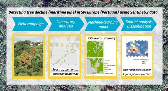
Workflow of the research project, which combines the analysis of field and satellite imagery for the development of a decline detection model focused on maritime pine occurring in Southwest Europe. PWN: Pinewood nematode; SAM: spectral angle mapper.
Figure 2.
Workflow of the research project, which combines the analysis of field and satellite imagery for the development of a decline detection model focused on maritime pine occurring in Southwest Europe. PWN: Pinewood nematode; SAM: spectral angle mapper.

Figure 3.
(A) Comparison of (unitless) normalized reflectance values (and standard deviation) of needles collected from healthy (green, n = 2140) and declining (red, n = 260) maritime pine trees. Samples were collected throughout the year and analyzed for the spectral range 400–1000 nm. (B) Sentinel-2 surface reflectance (490–2200 nm) of pixels containing healthy (green) and declining (red) maritime pine trees.

Figure 4.
Average needle reflectance and scans of a maritime pine tree with confirmed natural infection by Bursaphelenchus xylophilus (ITR49). Notice the pre-visual spectral changes noticeable in the spectra recorded on 25 July.
Figure 4.
Average needle reflectance and scans of a maritime pine tree with confirmed natural infection by Bursaphelenchus xylophilus (ITR49). Notice the pre-visual spectral changes noticeable in the spectra recorded on 25 July.

Figure 5.
Representative comparison of WorldView-3 (average) and Sentinel-2 (pixel) spectra for different percentages of decline cover across 3 key months in the wilting season (pre, -mid, and late-season). (A–C) Sentinel-2 reflectance for a pixel with 0% (green) and 43% (brown) canopy cover in decline. (D–F) Median WorldView-3 reflectance within the area covered by the Sentinel-2 pixel with healthy maritime pine trees. (G–I) Median WorldView-3 reflectance within the area covered by the Sentinel-2 pixel with declining maritime pine trees (43%) (Sentinel-2 and Worldview-3 imagery have different spectral ranges).

Figure 6.
Radar plot of the average values of selected indices (green line and shade: June data, healthy; brown line: November data, declining). The plot supported the identification of useful indices for further exploration and use in the Random Forest model (Compare with results of [19]). Index numbers can be found on Table 2.

Figure 7.
Receiving Operator Characteristics (ROC) curves for each class (A: declining; B: healthy).
Figure 7.
Receiving Operator Characteristics (ROC) curves for each class (A: declining; B: healthy).

Figure 8.
(Left): Output of the decline model applied to Sentinel-2 imagery (at the end of the 2018 decline season) and (Right): comparison with WorldView-3 True Color RGB. The location of declining trees can be detected visually in the high-resolution imagery (orange circles) and compared against the Sentinel-2-based detections.

Figure 9.
Histogram of false negative detections in Sentinel-2 imagery (2018/2019) as a function of percentage of decline symptoms in the canopy.
Figure 9.
Histogram of false negative detections in Sentinel-2 imagery (2018/2019) as a function of percentage of decline symptoms in the canopy.

Figure 10.
The number of detections in the Sentinel-2 model (declining trees), at a regional level, calculated for a reference tessellated hex grid for the 2020 season. Percent cover of conifers (mostly maritime pine) is represented as well as main roads, major population centers, and sawmills/wood depots (dark squares). S: Sertã; P: Proença-a-Nova; C: Cernache do Bonjardim (main urban centers).


Table 1.
Dates of acquisition of imagery used in the study for the development of the decline model and analysis of spectral trajectories.
Table 1.
Dates of acquisition of imagery used in the study for the development of the decline model and analysis of spectral trajectories.
| Sentinel-2 Imagery Dates | Worldview-3 Imagery Dates |
|---|---|
| 2017/06/14 (pre-study reference) | 2017/06/21 |
| 2018/06/19 (pre-season) | 2018/07/11 |
| 2018/07/29 (pre-season reference #1) | 2018/07/23 |
| 2018/09/22 (in-season #1) | 2018/09/11 |
| 2018/12/06 (late season #1) | 2018/12/06 |
| 2019/07/14 (pre-season reference #2) | 2019/07/15 |
| 2019/10/22 (in-season #2) | 2019/10/25 |
| 2020/01/05 (late season #2) | 2019/12/07 |
Table 2.
List of spectral indices calculated using the Sentinel-2 imagery and employed in the development of the decline detection model. Selected indices used to build the Random Forest model are listed.
Table 2.
List of spectral indices calculated using the Sentinel-2 imagery and employed in the development of the decline detection model. Selected indices used to build the Random Forest model are listed.
| Index Number | Index | Selected | Reference |
|---|---|---|---|
| 1 | CARI | [43] | |
| 2 | CI | Yes | [44] |
| 3 | CIAInt | [45] | |
| 4 | Datt | [46] | |
| 5 | EVI | [47] | |
| 6 | Gitelson2 | Yes | [48] |
| 7 | GreenNDVI | [49] | |
| 8 | Maccioni | Yes | [50] |
| 9 | MCARI | [51] | |
| 10 | MCARI2 | [52] | |
| 11 | mND705 | [40] | |
| 12 | mNDVI | [40] | |
| 13 | MPRI | [30] | |
| 14 | MSAVI | [52] | |
| 15 | mSR | Yes | [40] |
| 16 | mSR2 | Yes | [53] |
| 17 | mSR705 | Yes | [40] |
| 18 | MTCI | Yes | [54] |
| 19 | MTVI | [55] | |
| 20 | NDII | [56] | |
| 21 | NDVI | Yes | [57] |
| 22 | NDVI2 | Yes | [49] |
| 23 | NDVI3 | [58] | |
| 24 | OSAVI | [59] | |
| 25 | OSAVI2 | [60] | |
| 26 | PSND | [61] | |
| 27 | RDVI | [62] | |
| 28 | SAVI | Yes | [63] |
| 29 | SIPI | [64] | |
| 30 | SIPI+ | [64] | |
| 31 | SPVI | [65] | |
| 32 | TCARI | [55] | |
| 33 | TCARI_OSAVI | [55] | |
| 34 | TCARI2 | [60] | |
| 35 | TGI | [66] | |
| 36 | Vogelmann2 | [67] | |
| 37 | Vogelmann4 | [67] | |
| B4/B3 | Yes | ||
| NDVIpre–NDVImid-season | Yes |
Table 3.
Pigment values and Red Edge parameters for the needles represented in Figure 4 (June 2018 to January 2019).
Table 3.
Pigment values and Red Edge parameters for the needles represented in Figure 4 (June 2018 to January 2019).
| 24 June | 25 July | 2 October | 6 November | 3 January | |
|---|---|---|---|---|---|
| Chlorophyll-a+b (g·mL−1) | 1.1 | 0.84 | 0.41 | 0.07 | 0.08 |
| Carotenoids (g·mL−1) | 0.07 | 0.08 | 0.06 | 0.04 | 0.03 |
| Red Edge l0 (nm) | 675 | 671 | 668 | 660 | 660 |
Table 4.
Summarized performance results of the Sentinel-2 decline detection model, based on the assessment conducted using independent validation data.
Table 4.
Summarized performance results of the Sentinel-2 decline detection model, based on the assessment conducted using independent validation data.
| Class | Symptomatic | Healthy | Total (Map) | User Accuracy | Kappa | Mean Absolute Error (MAE) |
|---|---|---|---|---|---|---|
| Symptomatic | 274 | 64 | 338 | 81% | 0.79 | 0.053 |
| Healthy | 83 | 2779 | 2862 | 97% | ||
| Total (reference) | 357 | 2843 | ||||
| Producer accuracy | 77% | 98% | ||||
| Overall accuracy: | 95% | |||||
Publisher’s Note: MDPI stays neutral with regard to jurisdictional claims in published maps and institutional affiliations. |
© 2022 by the authors. Licensee MDPI, Basel, Switzerland. This article is an open access article distributed under the terms and conditions of the Creative Commons Attribution (CC BY) license (https://creativecommons.org/licenses/by/4.0/).
Share and Cite
MDPI and ACS Style
Mantas, V.; Fonseca, L.; Baltazar, E.; Canhoto, J.; Abrantes, I. Detection of Tree Decline (Pinus pinaster Aiton) in European Forests Using Sentinel-2 Data. Remote Sens. 2022, 14, 2028. https://doi.org/10.3390/rs14092028
AMA Style
Mantas V, Fonseca L, Baltazar E, Canhoto J, Abrantes I. Detection of Tree Decline (Pinus pinaster Aiton) in European Forests Using Sentinel-2 Data. Remote Sensing. 2022; 14(9):2028. https://doi.org/10.3390/rs14092028
Chicago/Turabian StyleMantas, Vasco, Luís Fonseca, Elsa Baltazar, Jorge Canhoto, and Isabel Abrantes. 2022. "Detection of Tree Decline (Pinus pinaster Aiton) in European Forests Using Sentinel-2 Data" Remote Sensing 14, no. 9: 2028. https://doi.org/10.3390/rs14092028
Note that from the first issue of 2016, this journal uses article numbers instead of page numbers. See further details here.