Determining the Influence of Long Term Urban Growth on Surface Urban Heat Islands Using Local Climate Zones and Intensity Analysis Techniques

Abstract

Urban growth, typified by conversion from natural to built-up impervious surfaces, is known to cause warming and associated adverse impacts. Local climate zones present a standardized technique for evaluating the implications of urban land use and surface changes on temperatures of the overlying atmosphere. In this study, long term changes in local climate zones of the Bulawayo metropolitan city were used to assess the influence of the city’s growth on its thermal characteristics. The zones were mapped using the World Urban Database and Access Portal Tool (WUDAPT) procedure while Landsat data were used to determine temporal changes. Data were divided into 1990 to 2005 and 2005 to 2020 temporal splits and intensity analysis used to characterize transformation patterns at each interval. Results indicated that growth of the built local climate zones (LCZ) in Bulawayo was faster in the 1990 to 2005 interval than the 2005 to 2020. Transition level intensity analysis showed that growth of built local climate zones was more prevalent in areas with water, low plants and dense forest LCZ in both intervals. There was a westward growth of light weight low rise built LCZ category than eastern direction, which could be attributed to high land value in the latter. Low plants land cover type experienced a large expansion of light weight low rise buildings than the compact low rise, water, and open low-rise areas. The reduction of dense forest was mainly linked to active expansion of low plants in the 2005 to 2020 interval, symbolizing increased deforestation and vegetation clearance. In Bulawayo’s growth, areas where built-up LCZs invade vegetation and wetlands have increased anthropogenic warming (i.e., Surface Urban Heat Island intensities) in the city. This study demonstrates the value of LCZs in among others creating a global urban land use land cover database and assessing the influence of urban growth pattern on urban thermal characteristics.

1. Introduction

Urban areas continue to expand in population and built-up extent, with faster rates in developing countries [1,2,3,4,5,6]. Whereas urban growth is often considered as a sign of economic vitality [3], its adverse impacts that include increased air pollution, Surface Urban Heat Islands, dust and haze, significantly influence urban micro- and macro-climate and affect urban environmental quality and human health [7,8]. Globally, urbanization has caused climate modifications, most evident in higher temperatures in urbanized than the non-urbanized surroundings [9,10,11,12,13]. Such growth often exacerbates heat stress in the already warming (due to global climate change) urban areas, leading to deterioration of outdoor thermal comfort [14]. Urban growth and associated surface changes induce near-surface warming, which increases energy and water demand due to search for indoor and outdoor thermal comfort [15,16,17,18]. Hence, urban growth assessment techniques that consider both surface and near surface characteristics and atmospheric gas/pollutant emissions are valuable in determining the influence of anthropogenic processes on the urban thermal emissions to inform sustainable urban growth.

Remote sensing offers a variety of data for analyzing spatial and temporal effects of urban land surface changes on the urban thermal environment. This has largely been facilitated by advances in sensor development that has improved the quality and availability of remotely sensed data. For instance, missions such as Landsat offer large archival data spanning as far back as 1972 at reasonable and improved radiometric, spectral and spatial resolution, valuable for assessing both large scale and localized temporal and multi-temporal landscape and environmental patterns [19,20,21,22,23]. A large body of literature has investigated the impact of land use land cover (LULCs) changes on surface and near surface temperature, e.g., Kumar and Shekar [24] and Uddin et al. [25]. These studies have indicated that impervious, bare and built-up surfaces result in urban warming while vegetation and water bodies act as thermal sinks. However, whereas LULC-based techniques and surface characterization schemes account for the contributions of land surface changes to temperature dynamics, they often exclude other anthropogenic contributions such as emission, which are key drivers of temperature changes associated with urban growth. Hence, schemes that account for both land surface characteristics and gas emissions/pollutants as drivers of changes in the thermal environment are necessary to adequately explain climatic changes in such complex environments.

Due to the dependence on LULC schemes, studies on effects of urbanization on temperature have mostly defined Surface Urban Heat Island (SUHI) as the difference between “urban” and “rural” temperature [26,27,28,29,30,31]. In such studies, rural and urban are vaguely defined by differences in population and built-up extent in a manner that is not universal [32,33,34]. However, this separation is no longer always clear cut as traditional and non-traditional urban and rural land uses increasingly continue to coexist [33]. The traditional classification scheme is area specific, making it difficult to make global comparisons as LULC characteristics vary between cities of the same country and between countries. However, analysis based on Local Climate Zones (LCZ) provide understanding of urban structures and land uses in a globally standardized manner, useful for understanding the influence of urbanization on urban climate [33,34,35]. The LCZ scheme is local and climatic in nature considering surface cover, three dimensional surface structures (such as height and density of buildings and vegetation) as well as anthropogenic thermal emissions [8,35,36,37,38,39]. LCZs provide useful information for assessing adherence of cities to the 2030 agenda for sustainable development Goal 11 [40] both in the form of LULC transitions and anthropogenic emissions effects on climate. Hence, LCZ provide a standard basis upon which the impacts of urban growth on the thermal environment can be monitored and assessed.

The LCZ scheme emphasizes the difference in temperature among the categories within and between cities, thus directly linked to climate of an area, while contributing to the creation of the global urban database [11,32]. Close association between LCZ and LST shows that LCZs are helpful for examination of evolution of SUHI over time [41]. LCZs are more conducive to analysis and less prone to confusion because they highlight common exposure characteristics and invite physically based explanations of SUHI magnitude [42,43,44,45,46,47,48,49]. Studies which used LCZs in SUHI analysis mostly focused on short temporal scales such as diurnal, seasonal and annual, e.g., United Nations General Assembly [40] and Ardiyansyah et al. [49]. Focus on long term interactions between LCZs and SUHI have remained understudied, especially in Africa. Furthermore, although Stewart and Oke [33] showed the effectiveness of LCZs in defining SUHI in cities, application of inter-LCZ temperature difference to define SUHI has remained minimal, especially in the analysis of long-term changes. Most of the studies that analyzed the relationship between LCZs and SUHI either used LST to directly represent SUHI [33,46,49], reclassified LST into different SUHI categories [45], converted LST into other forms such as Distribution Index [41] or normalized temperatures [47,50], or used urban to rural temperature gradient [29,48,51,52]. Of the few studies that used temperature difference between LCZ types to quantify SUHI, most of them used the Low plants LCZ as a reference against which LSTs of other LCZs were compared [50,53,54,55]. A number of studies on LCZ have mainly focused on the current state and short-term variations as well as contributing to World Urban Database and Access Portal Tool (WUDAPT), e.g., Cai et al. [32], Cai et al. [36], Danylo et al. [37], Qiu et al. [39], and Demuzere et al. [56], with little effort towards understanding and explaining their long term changes that affect a city’s SUHI intensity. In long term analysis, single date imageries are commonly used to develop static LCZ for each year, ignoring the value of combining multi-seasonal data for the same analysis. Long term changes provide a better understanding of the contribution of human activities to local climate change and assessment of adherence of city growth patterns to Agenda 2030 for Sustainable Development Goal 11 [39]. Hence, there is a need to use multi-season imageries to generate LCZ and LCZ-based SUHI to determine long term effects of urban growth on a city’s thermal environment.

Cities in developing countries have been experiencing growth characterized by massive changes in land surface characteristics and intensification of activities, which have the potential to pollute the atmosphere and exacerbate changes in local thermal environments. Although the trends have been observed in different parts of the world, actual changes vary between and within countries, triggering the need for detailed and city-specific assessments. Hence, in-depth understanding of a city’s specific influences on LCZ is important for ensuring that further development is climate smart and sustainable. However, available literature on long term LCZ changes [52,57,58,59] uses the traditional “from to” change detection approach which lacks in depth analysis to provide detailed understanding of long term LCZ transitions and their potential impacts on local climate. Although not yet applied to understand long term LCZ transitions, in depth analysis of changes based on transition matrices of different periods is better done using intensity analysis than the traditional “from to” change detection approach. Intensity analysis is useful for effecting classifications of different time intervals to understand sizes and intensities of temporal changes among categories [60,61,62,63], as it provides details on whether transition from one category to another deviates from a uniform process [61]. It also identifies time intervals when rate of change was fast or slow, identifies whether category changes were active or dormant in a time interval and whether a category was targeted or avoided by changes during an interval [62,64,65]. Furthermore, it analyzes land changes relative to size of category to identify systematic transitions over time [62]. As such, it reveals information such as underlying processes associated with changes which ordinary change detection conceals [66]. For instance, Alo and Pontius [67] revealed that protected areas in Ghana experienced systematic transitions from closed forest to bare and bush fires, while Ekumah et al. [66] revealed that between 1985 and 2017, human induced LULCs grew at the expense of natural categories in the Densu Delta, Sukumo II and Muni Pomodze Ramssar sites in Ghana. Intensity analysis is thus valuable for obtaining an in-depth and detailed analysis and understanding of long term LCZ changes, especially for cities such as Bulawayo where spatial and temporal temperature patterns are not yet documented. Combining intensity analysis and SUHI retrieval in the context of LCZ will therefore provide a detailed understanding of the effect of urban growth patterns on the thermal environment of cities.

Hence, the aim of this study was to integrate intensity analysis and LCZ-based SUHI retrieval to provide detailed analysis of the impact of urban growth on the thermal environment in Bulawayo metropolitan city in Zimbabwe. Specifically, this study sought to determine long term effect of urban growth on the thermal environment using LCZ between 1990 and 2020 in Bulawayo city, Zimbabwe. The study also utilized intensity analysis for an in-depth assessment of the changes in LCZ in Bulawayo between 1990 and 2020. Additionally, and contrary to the broad literature that uses the between rural–urban difference in temperature, this study enhanced the use of inter-LCZ temperature difference approach to quantify SUHI intensity and their long term changes.

2. Methodology

2.1. Description of the Study Area

Bulawayo is the second largest city in Zimbabwe (Figure 1). It is located to the southeast of the country (Figure 1a) at an elevation of approximately 1358 m above sea level. The period between October and March is hot and wet with a minimum of 16 °C and maximum of 30 °C, with an average temperature of 25 °C, while the rest of the year is cool and dry, with a minimum of 10 °C, maximum of 25 °C and average temperature of 15 °C [68]. Generally, the area receives erratic rainfall, with annual average precipitation of 600 mm that ranges from 199.3 mm to 1258.8 mm, typical of a semi-arid climate. Bulawayo (Figure 1b) lies in the subtropical steppe (Bsh) according to Koppen climate classification. The period from December to February is the wettest. Most rain falls from December to February and the area is vulnerable to droughts due to proximity to the Kalahari Desert [69,70].

2.2. Field Observations of Local Climate Zones in Bulawayo

Since the WUDAPT places little emphasis on field data collection, a survey to identify and obtain ground truth samples of LCZ categories in the study area was important to guide digitizing of training polygons in Google Earth Field observations, which allowed for identification of inter- and intra-category variabilities that could not be adequately captured from Google Earth. The sample coordinates of each LCZ category (ground truth data) were obtained between 18 and 27 October in 2020. This experience also guided selection of training areas for the historical periods using Google Earth in the absence of field measurements for that period. Field observations increased the validity of the analysis instead of exclusive reliance on Google Earth retrievals. Generally, 8 LCZ categories were identified in the study area that fit into the description of LCZs provided by Stewart and Oke [33]. The categories were three land use-based LCZs, namely Compact low rise (LCZ3), Open low rise (LCZ6) and Light weight low rise (LCZ7), as well as three land cover-based LCZs, which were Dense forest (LCZA), Low plants (LCZD) and Water (LCZ G). The study used LCZs definitions and pictorials provided by Stewart and Oke [33] as reference to identify similar classes in the study area for global comparability.

2.3. Multi-Temporal Remotely Sensed Datasets

Multi-temporal Landsat 5, Landsat 7 and Landsat 8 Operational Land Imager datasets were downloaded from the United States Geological Survey’s (USGS) earth explorer website for analysis. Cloud free imageries for the wet and dry vegetation periods were downloaded to minimize compromising effects of atmospheric noise on image radiometric values and LCZ mapping accuracy.

Table 1. Multi-temporal and multi-spectral remote sensing imagery used in the study.

Imagery	Date	Season	Days to Recent Precipitation before Overpass (Days)	Rainy Days in 10 Days before Overpass (Days)	Precipitation in 10 before Overpass (mm)
Landsat 5	27 April 1990	Post rain	1.0	1.0	4.8
Landsat 7	12 April 2005	Post rain	4.0	6.06	13.1
Landsat 7	21 April 2020	Post rain	1.0	10.0	16.9
Landsat 5	14 June 1990	Cool	27.0	0.0	10.0
Landsat 5	7 June 2005	Cool	22.0	0.0	0.0
Landsat 7	24 June 2020	Cool	2.0	4.0	1.4
Landsat 5	20 October 1990	Hot	1.0	1.0	7.0
Landsat 7	21 October 2005	Hot	99.0	0.0	0.0
Landsat 8 OLI	15 October 2020	Hot	3.0	5.0	6.5

shows the imageries used for 1990, 2005 and 2020. In this study, Landsat thermal, panchromatic as well as bands for monitoring cirrus clouds and coastal aerosols were not used for analysis. For each year, dry and wet periods were selected in order to capture seasonal variations in LCZ, especially in areas with vegetation. The post rain period was chosen to represent the wet biomass period because during that period, trees and grasses are vibrant after a rainy season. The rainy season was avoided to attain both temporal and multi-temporal cloud free imagery. Amorim [71] indicated that Surface Urban Heat Island intensity is influenced by responses of vegetation to rainfall patterns before the imagery date. Amorim [71] observed that Heat Island Intensities increased during periods of high biomass, which reduce temperatures in vegetation areas. Therefore, precipitation patterns of up to 10 days prior to overpass (amounts and rainy days) are shown in Table 1. Generally, the number of rainy days prior to overpass was higher in the post-rain than other seasons, with the lowest number in the cool season. Cumulative rainfall amounts in 10 days before overpass were also low in all seasons (less than 20 mm).

2.4. Mapping of LCZ Using Dry and Wet Season Imagery

The advantage of the LCZ scheme is that their mapping follows an easy and standardized approach for mapping LCZ, which involves downloading of imagery, digitizing of training sites (for classification and accuracy assessment) on Google Earth and supervised classification using the random forest (RF) classifier [37,72,73]. Local Climate Zones for Bulawayo were thus mapped following the WUDAPT L0 procedure [8,36,56,73,74]. The procedure involves downloading suitable imagery of the study area, on-screen selection and digitizing of training areas on Google Earth, supervised image classification using the Random Forest (RF) Classifier and post classification accuracy assessment in SAGA GIS. The procedure was adopted due to its use of readily available and freely downloadable imageries as well as easy access to the SAGA GIS software for implementation. Additionally, the steps have been followed in different parts of the world, making it very easy to follow. Use of the RF classifier makes the procedure attractive as it can perform bootstrapping analysis which is used to assess quality of the LCZ database [56,75]. The RF model is a collection of decision trees and each tree is made up of a subset of training dataset for a subset of predictors [73,76,77]. It is termed RF because its subsets are randomly formed. In RF classification, the predicted value is the mode of the predictions from all trees. Main advantages of RF are the use of both categorical and numerical values, the evaluation of the precision of prediction, the robustness in the presence of outliers, noise, and overfitting. The RF model can quantify the contribution of each predictor to the total spatial variability of the target and assigns a variable importance score to each predictor. Random forest requires a small amount of training data, yet provides competitive results and can handle a large volume of input data without deletion, while still capable of identifying important variables for classification [78,79,80,81,82,83]. In addition, RF is not sensitive to over-training or noise and is desirable for multi-source remote sensing and geographical information systems data [75,81]. LCZ maps were produced for the years 1990, 2005 and 2020 using the same training areas. These were collected from locations whose LULC category did not change over time in order to eliminate the effect of differences in ground truth data on mapping accuracy. The use of the same training areas was made possible by availability of historical Google Earth imagery where the areas could be clearly identified at different periods. In order to adhere to the definition of LCZ, which requires that they cover at least a hundred meters to several kilometers to influence temperature [8,11,41], the maps were resampled using a 5 by 5 pixels window. A LCZ must be large enough to influence temperature of an area. In order to quantify the effect of seasonality on mapping accuracy, LCZ maps were also produced using data for the hot and dry season for comparison with analysis based on a combination of data from the post rain, cool dry and hot dry periods. Figure 2 provides a summary of the procedure followed. The broken arrow in the figure shows the approach taken by previous studies which largely skip the iterative step of qualitative accuracy assessment, further improving accuracy before change detection.

2.5. Accuracy Assessment

The WUDAPT procedure automatically splits training areas into 50% for classification and 50% for accuracy assessment. A confusion matrix is formulated in a tabular form for the purposes of comparing reference class labels (ground truth) with labels for corresponding pixels on a derived classification of remote sensing imagery [83]. The diagonal values on the matrix indicate where categories assigned on the classified map correctly corresponded with ground truth. For example, the matrix shows the number of pixels which were assigned same LCZ value as observed on the ground as well as those that are misallocated following classification of remote sensing data. The confusion matrix was used to generate indicators of accuracy at class level (Producer Accuracy and User Accuracy) as well as at entire study area level (Overall Accuracy—OA—and Kappa—K). The use of OA and K with the inclusion of ground data is the most common and reliable way of assessing accuracy [84]. Accuracy assessment is important for the separation of real changes from changes due to errors for LCZ maps of different periods. Error analysis was done for all the study years. Accuracy was also assessed qualitatively by overlaying the produced LCZ maps with a corresponding Google Earth imagery in combination with expert judgement. The number of training areas was objectively and iteratively increased in areas where marked mismatches were observed to capture for intra- and inter-class variabilities using Google Earth.

2.6. Detection of Long-Term Changes in LCZ in Bulawayo

A 30-year period (1990 to 2020) was selected, as the study aimed at using LCZ dynamics as a proxy for temperature changes in Bulawayo. The World Meteorology Organization (WMO) recommends a minimum of 30 years for a representative climate change analysis. The period was further split into two 15 year periods (i.e., 1990 to 2005 and 2005 to 2020) for understanding of rapid changes that occur at local scale and for intensity analysis purposes. Additionally, Coppin and Bauer [85] recommended a period of at least 3 years for change detection involving forests and other vegetation types. In an urban setting, there is a mix of rapid and slow LCZ making a period of at least 15 years enough to detect effect of all change trajectories on the climate of an area. A post classification change detection approach was used. The approach produces a change matrix/table which shows the number of pixels which were converted to other LCZ types or remained in the same categories in the considered interval. For instance, the table indicated the number of pixels which were in LCZ1 at the beginning and remained in the same as well as those that were changed to other LCZ categories during the same time interval. Although the change matrix is useful in depicting the quantities and directions of change, it does not adequately explain the changes [60,85,86], hence the need for intensity analysis.

2.7. Intensity Analysis for In-Depth Characterization of LCZ Changes

Intensity analysis was used to obtain a better understanding of LCZ transitions between 1990 and 2020 in Bulawayo. It was used to assess locations and intensities of temporal changes among categories. The analysis was done at the interval, category and transition levels [87,88,89,90] using freely available software on Pontius Clarke University web page (https://www2.clarku.edu/faculty/rpontius/ (accessed on 15 April 2021)). The site provides an easy to use Excel sheet where the change matrix for a given time interval is entered. Varga et al. [91] provide descriptions and defining equations used in the analysis that were adopted in this study.

2.7.1. Interval Level Intensity Analysis

Interval level was used to determine overall changes per time period for the 1990 to 2005 and 2005 to 2020 time intervals. Overall changes in the interval 1990 to 2005 were compared with those for the interval 2005 and 2020. This was important to identify which interval had changes characterized as fast or slow. The change percentage for an interval t is defined as in Equation (1) [91]:

$$S_t=\frac{\left(size of changes during interval t\right)\times 100\%}{size of studyarea in which changes are occurring}$$

(1)

S_t is the uniform intensity in interval t. An interval change is fast if it exceeds uniform intensity and slow if otherwise.

2.7.2. Category Level Analysis

Changes in gross loss or gain in intensity among different categories was described by category level intensity analysis during time interval t (where t separately represents the two interval periods—1990 to 2005 and 2005 to 2020). Category level loss (L_ti) and gain (G_tj) during the interval t are obtained using Equations (2) and (3) as

$$L_{ti}=\frac{\left(size of loss of category i during interval t\right)\times 100}{size of i at the start of interval t}$$

(2)

$$G_{tj}=\frac{\left(size of gain of category j during interval t\right)\times 100}{size of category j at the end of interval t}$$

(3)

According to [64], calculation of category persistence (P_ti) is done using Equation (4):

$$P_{ti}=\frac{\left(size that has maintained category i during interval\right)\times 100\%}{size of spatial extent}$$

(4)

$S_t=L_{ti}=G_{tj}$ for all categories i and j if changes are uniformly distributed across spatial extent. Uniform transition assumes category i uniformly changes to other categories during the time interval. If $L_{it}>S_t$ then the loss of category i is active in the interval t while loss is dormant if $L_{it}<S_t$. Dormant implies that the loss of category i slowed down or stopped within the interval t. Similarly, gain of category j in the interval t is active if $G_{tj}>S_t$ and dormant if $G_{tj}>S_t$. When two intervals are considered and the status of a change as dormant or active is same in both intervals, then the category’s loss or gain is said to be stationary.

2.7.3. Transition Level Analysis

The analysis describes the variation in intensity with which the gain of a particular category transitions from other categories within a time interval [60]. Transition level intensity analysis was used to determine whether change of a category avoids or targets other categories. If the intensity of the change from category i to category j exceeds uniform intensity, then category i targets j otherwise it avoids.

2.7.4. Retrieval of Changes in SUHI in Response to Long Term LCZ Dynamics

Thermal data of Landsat 5, 7 and 8 were used to compute land surface temperature (LST) for 1990, 2005 and 2020. Initially, the data were corrected of differences in solar zenith angles. While Landsat 8 has two thermal infrared bands, a single channel technique was applied for all the periods to minimize effects of differences in computation algorithms on LST variations between time periods. Digital numbers of thermal data were converted to radiances, which were then used to determine brightness temperature (T_b) and surface temperature (T_s) using Equations (4) and (6), respectively [91,92,93,94].

$${\mathrm{T}}_{\mathrm{b}}=\frac{{\mathrm{K}}_2}{\ln \left(\frac{{\mathrm{K}}_1}{{\mathrm{L}}_{\mathsf{\lambda }}}+1\right)}$$

(5)

where K₁ takes a values of 607.76, 666.09 and 774.89 W/(m² srμm), while K₂ has values of 1260.56, 1282.71 and 1321.08 W/(m² srμm), using Landsat 5, Landsat 7 and Landsat 8 data, respectively. A method based on spectral and blackbody radiance of the thermal infrared band was used to obtain pixel-based land surface emissivity map ($\mathsf{\epsilon }$) [95]. Emissivity correction was applied on brightness temperature to obtain actual land surface temperature using Equation (6) [96].

$${\mathrm{T}}_{\mathrm{s}}=\frac{{\mathrm{T}}_{\mathrm{B}}}{1+\left(\frac{{\mathsf{\lambda }\mathrm{T}}_{\mathrm{B}}}{\mathsf{\rho }}\right)\ln \mathsf{\epsilon }}$$

(6)

where $\mathsf{\lambda }$ is the central wavelength of emitted thermal radiance (11.5 μm for Landsat 5 and Landsat 7 and 10.9 μm for band 10 of Landsat 8) and $\mathsf{\rho }$ is equal to 1.438 × 10⁻² mK. The procedure above was used to retrieve LST on two different dates so that independent sets were used for training and accuracy assessment of the developed estimation algorithm. The spatial structure of LST intensities were used for visual and quantitative analysis of changes which occurred between 1990 and 2020.

Stewart and Oke [33] defined SUHI as the difference in LST between LCZs. In this study, we adopted an approach by Dimitrov [97], which defined SUHI as the maximum temperature difference between LCZs. For each year, the Surface Urban Heat Island was computed as the difference between the average T_s of LCZ category and the mean surface temperature of the water LCZ (LCZ G), which was identified as giving the highest LST difference with other LCZs consistently in all years using Equation (7).

$${\mathrm{SUHI}}_{\mathrm{LCZ}}={\mathrm{LST}}_{\mathrm{LCZ}\mathrm{X}}-{\mathrm{LST}}_{\mathrm{LCZ}\mathrm{Y}}$$

(7)

SUHI_LCZ is the SUHI derived from LST difference between other LCZs (X) and the Water LCZ (Y). Although studies such as Stewart and Oke [33] used LCZ D as reference, it was not applicable in this study due to the varying and opposing effects of the LCZ in different places and seasons for daytime analysis. For instance, agricultural areas had thermal values that vary in space and time and between seasons, rendering them as heat sinks in some instances and heat sources in others. As such, during the growing season, they acted as heat sinks while in the dry season, their heat mitigation value was reduced. In other areas, they were completely removed, as they turned to dry biomass or bare soil areas. Similarly, grasslands (also in LCZ D) vary in heat mitigation value depending on season and maintenance, making them another example of inconsistency of LCZ D. The LCZ G was chosen as a reference since it was the coolest and more stable than the vegetation based categories, which have broad seasonal and long term variations in characteristics. Mean LST per LCZ category was obtained using the Zonal Statistics overlay function in ArcGIS version 10.2 for each year. Changes in SUHI per LCZ strata were monitored and linked with observed changes in LCZ from 1990 to 2020 in 15-year intervals.

3. Results

3.1. LCZ Maps Based on Multi-Seasonal Image Analysis

The use of imagery for the wet and dry vegetation periods reduced the confusion between light weight low rise and low plants in the western areas (Figure 3). The overall classification accuracies were 98%, 98.2% and 95%, for 1990, 2005 and 2020, respectively. Visual inspection shows that between 1990 and 2020, light weight low rise LCZ was spread westwards into areas formerly occupied by low plants. All built local climate zones increased in spatial coverage while low plants and dense forest LCZ decreased in coverage. The water LCZ also decreased in coverage during the study period.

Compact low rise increased by 4.33 km² between 1990 and 2005 and by 2.50 km² between 2005 and 2020 (

Table 2. Coverage of LCZ categories in 1990, 2005 and 2020.

LCZ Category	Coverage of LCZ Categories in km2 (% in Bracket)
	1990	2005	2020
Compact low rise	12.84 (3.0)	17.17 (4.0)	19.67 (4.5)
Dense Forest	38.41 (8.9)	41.32 (9.5)	26.07 (6.0)
Light weight low rise	39.60 (9.1)	60.87 (14.0)	75.12 (17.3)
Open low rise	45.13 (10.4)	74.00 (17.1)	88.56 (20.4)
Water	2.06 (0.5)	1.45 (0.3)	1.26 (0.3)
Low plants	295.42 (68.2)	238.66 (55.1)	222.77 (51.4)

). Similarly, light weight low rise expanded by 21.27 km² between 1990 and 2005 and by 14.25 km² between 2005 and 2020. The open low rise LCZ also showed the same pattern of larger increase in the 1990 to 2005 interval than in the 2005 to 2020 interval. On the other hand, the expansion rate of dense forest between 1990 and 2005 (2.91 km² in 15 years) was smaller than the depletion rate of the LCZ between 2005 and 2020 (15.25 km² in 15 years). Low coverage diminished faster in the 1990 to 2005 interval than in the 2005 to 2020 interval.

3.2. Changes in LCZs for Bulawayo Using Multi-Temporal (Dry and Wet) Datasets

Table 3. LCZ changes from 1990 to 2020 in Bulawayo.

LCZ Category	LCZ Category Changes in km2 (% in Bracket)
	1990 to 2005	2005 to 2020	1990 to 2020
Compact low rise	4.33 (33.7)	2.50 (14.6)	6.83 (53.2)
Dense Forest	2.91 (7.6)	−15.26 (−37.0)	−12.35 (−32.1)
Light weight low rise	21.27 (53.7)	14.27 (23.5)	35.54 (89.7)
Open low rise	28.88 (64.0)	14.50 (19.7)	43.43 (96.2)
Water	−0.61 (−29.8)	−0.19 (−13.2)	−0.81 (−39.1)
Low plants	−56.77 (−19.2)	−15.89 (−6.7)	−72.66 (−24.6)

shows that Compact low rise increased by 1.5% between 1990 and 2005 and a further 2.2% between 2005 and 2020, giving a 30-year expansion of 3.7%. A significant decrease in coverage was observed in the dense forest LCZ, which experienced a net reduction of 42% between 1990 and 2020, with greater change in the 1990 to 2005 than 2005 to 2020 periods. Generally, all built-up LCZ increased in coverage between 1990 and 2020, with larger expansion in the light weight low rise than other built-up LCZs. Sustained contraction was recorded in dense forest and water LCZs. The low plants LCZ, which in this study included croplands, grasslands and parks increased by 4.3% over the entire period, except a 0.9% decrease recorded between 2005 and 2020.

3.3. Intensity Analysis

3.3.1. Category Level Intensity Analysis for 1990 to 2005 and 2005 to 2020 Intervals

All other LCZs except compact low rise were gainers or losers in the 1990 to 2005 and 2005 to 2020 intervals (Figure 4a,b). The gain in Compact low rise LCZ was dormant in the 1990 to 2005 interval, implying the gain stopped or slowed along the interval. In the interval 2005 to 2020, the gain of compact low rise was active in the 2005 to 2020 interval. Low plants were active losers in the 1990 to 2005 interval and became dormant losers (the loss of the class was slow or stopped along the interval) in the 2005 to 2020. The water LCZ was an active loser in both intervals. The light weight low rise LCZ was a dormant gainer in the initial interval, but turned into an active gainer in the interval 2005 to 2020.

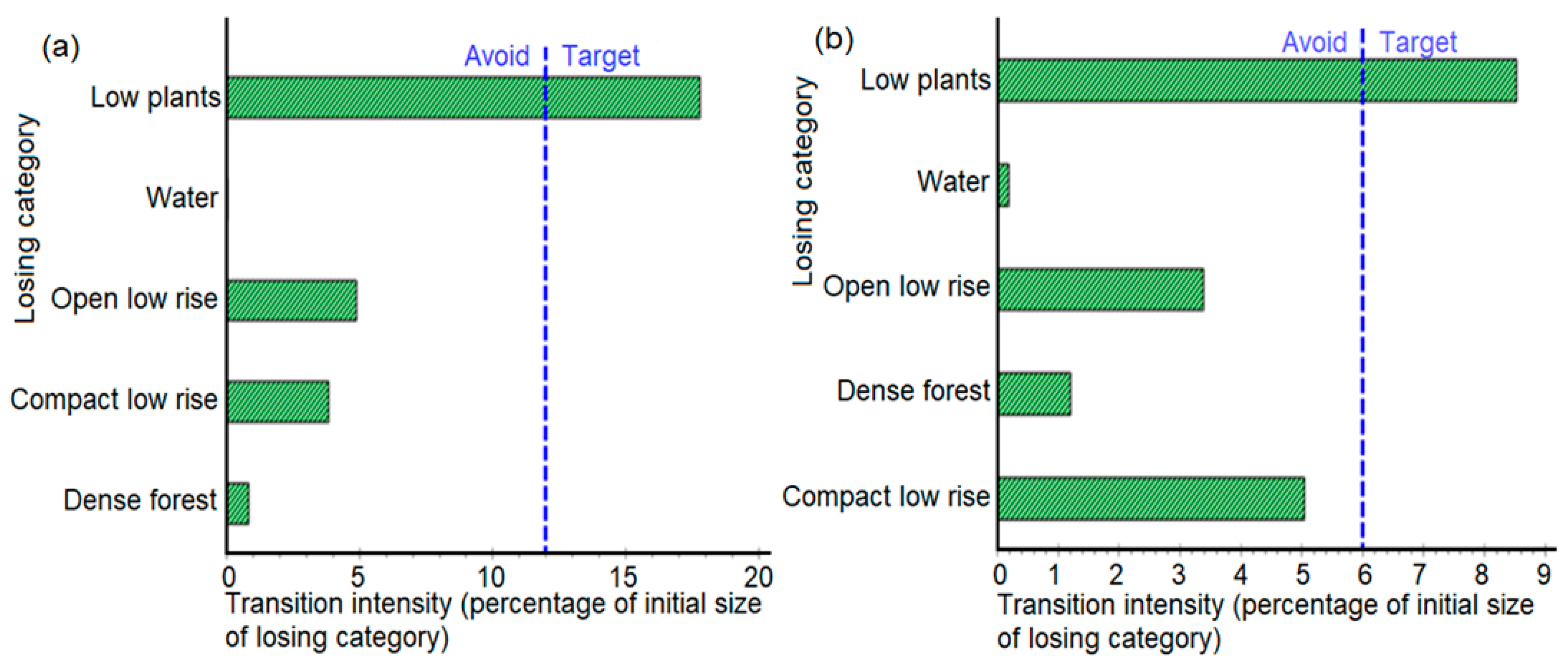
3.3.2. Transition Intensity of Gaining Categories Encroaching into Losing Categories

The expansion of compact low rise LCZ targeted water, open low rise and light weight low rise between 1990 and 2005 with open low rise LCZ as the most intensely targeted (Figure 5a). The growth of compact low rise avoided low plants and vegetation LCZs during the same period. In the 2005 to 2020 interval, the Compact low rise LCZ continued to target open low rise and lightweight low rise areas (Figure 5b). The intensity of transition of water to compact low rise was greater in the interval 1990 to 2005 than 2005 to 2020. In both intervals, the gain of compact low rise avoided low plants and dense forest LCZ areas.

The gain of light weight low rise between 1990 and 2005 targeted low plants and avoided dense forests and open low rise water and compact low rise LCZ areas (Figure 6a). Between 2005 and 2020, the gain of Light weight low rise LCZ continued to target low plants while avoiding other LCZs (Figure 6b).

The gain of the dense forest LCZ in the 1990 to 2005 interval targeted low plants (Figure 7a). This could imply growth of trees in grasslands such as parks in addition to other tree planting efforts. The expansion of low plants LCZ targeted dense forest, open low rise and light weight low rise, while it avoided water and compact low rise in the 2005 to 2020 interval (Figure 7b). The study also noticed slight spectral confusion between light weight low rise and low plants, especially in the western parts of the study area.

The gain of open low rise LCZ in the 1990 to 2005 interval targeted low plants (Figure 8a), while in the interval 2005 to 2020 it targeted low plants, water, dense forest and compact low rise (Figure 8b). The gain targeted dense forest more than low plants LCZ, which could be due to the nature of the LCZ that consists of a few and well-spaced buildings surrounded by trees and grass. Expansion into water reveals an adverse environmental impact, with growth intrusion into wetland areas.

3.4. Long Term Changes in the Two Dimensional LST in Response to LCZ Changes

Figure 9 shows expansion of high temperature surfaces between 1990 and 2015. In 1990, LSTs in the 37.8 to 43.8 °C range (Figure 9a) dominated the city, while LSTs below 43.8 °C became uncommon in 2005 (Figure 9b). Visual inspection shows that in 2020, the LSTs became even higher, with most areas recording values above 46.8 °C (Figure 9c). The water areas were the most stable, with LSTs in the 16.8 to 37.8 °C range in 1990, 2005 and 2020.

In each year, SUHI intensities between the Compact low rise and Low plants LCZs were comparable, although in 2020 the Low plants were slightly warmer (Figure 10). SUHI intensities increased with built-up density as well as density of tall buildings evidenced by largest intensity in Compact low rise (e.g., 11.7 °C in 2020) and lowest in Open low rise (10 °C). Dense vegetation LCZ areas were cooler than built LCZ in all the periods.

4. Discussion

Mapping accuracy was very high, exceeding 95% for 1990, 2005 and 2020 LCZ maps. Accuracy of at least 95% in LCZ mapping were also recorded by Danylo et al. [37] in Kyiv and Lviv in Ukraine for city specific analysis, which was higher than the below 75% accuracy they achieved using training data for multiple city mapping. The differences in accuracy between city level and large scale LCZ mapping approaches demonstrate that better LCZ maps are generated with city specific efforts than when training areas of another city are used for LCZ mapping [55]. The high accuracy achieved stresses the high performance of random forest classifier in comparison to other classifiers such as support vector machine [75,80,81,83]. RF uses a set of classifiers that make it superior to individual classifier based approaches [81]. The use of multi-seasonal data also enhanced discriminability of LCZs in this study, which resulted in high yearly accuracies. LCZ maps did not show most of the linear features such as roads and rivers due to the large filter used. As noted by Kotharkar and Bagade [8] and Gal et al. [72], an LCZ must be large enough to affect an area’s temperature, while use of a large filter removes linear features and expands urban area. According to Kotharkar and Bagade [8] and Gal et al. [72], shifting to a coarser scale results in loss of a number of LCZs.

Consistent with global trends, there was a general increase in built LCZ in Bulawayo between 1990 and 2020. This is a characteristic of city growth globally typified by conversion from natural land covers to urban fabric. For instance, in Kigali, Rwanda, Akinyemi et al. [60] observed an increase in built area from 1% in 1981 to 19% in 2002, followed by a slight decrease to 18% in 2014. Similar to Bulawayo, and indeed other global cities trends, Akinyemi et al. [60] showed a general increase in built-up area over a 33 year period. Whereas the expansion of Built LCZ continued throughout the study period, it was faster between 1990 and 2005 than between 2005 and 2020. For instance, expansion of compact low rise, which coincides with the Central Business District, was slower than other built LCZs in both intervals. Between 1990 and 2020, lightweight low rise LCZ expanded faster than other built LCZ. Generally, in Bulawayo, other built LCZ grow around the Central Business District with light weight low rise spreading to the west and spacious built-up LCZ spreading to the east. This limits space for further expansion of the Central Business District (CBD), which explains slowed growth of the corresponding LCZ between 2005 and 2020.

All other LCZs were gainers or losers in the 1990 to 2005 and 2005 to 2020 intervals, except compact low rise LCZ that was dormant in the 1990 to 2005 interval, implying the gain stopped or slowed along the interval. In the 2005 to 2020 interval, the gain of compact low rise was active. Low plants were active losers in the 1990 to 2005 interval and became dormant losers (the loss of the class was slow or stopped along the interval) in the 2005 to 2020. The water LCZ was an active loser in both intervals. The light weight low rise LCZ was a dormant gainer in the initial interval, but was an active gainer in the 2005 to 2020 interval. Sustained contraction was recorded in dense forest and water LCZs. The low plants LCZ, which in this study included croplands, grasslands and parks increased over the entire period (by 4.3%), although they experienced a decrease (by 0.9%) between 2005 and 2020. This shows that although the LCZ had expanded due to activities such as deforestation, it was affected by the expansion of built-up between 2005 and 2020.

The expansion of built LCZs between 1990 and 2005 was most prevalent in the open low rise LCZ. The growth of compact low rise avoided low plants and vegetation LCZs during the 1990 to 2005 period. In the interval 2005 to 2020, the Compact low rise LCZ continued to target open low rise and lightweight low rise areas. This may signify growth of the industrial and CBD to serve the surrounding residential areas, which were also expanding. The intensity of transition of water to compact low rise was greater in the interval 1990 to 2005 than 2005 to 2020. In both intervals, the gain of compact low rise also avoided low plants and dense forest LCZ areas. This may signify adherence to the Environmental Management Act, which was signed into law in 2013 [98]. The Act has increased protection of wetlands and the general environment with non-compliance, especially of business enterprises attracting heavy fines. Avoidance of water areas by expansion of compact low rise may also be a result of costs associated with construction in wetlands.

The gain of light weight low rise between 1990 and 2005 targeted low plants and avoided dense forests, open low rise water and compact low rise LCZ areas. Between 2005 and 2020, the gain of Light weight low rise LCZ continued to target low plants while avoiding other LCZ. The shift from low plant to light weight low rise indicates the change from primary production to industry based economy as the city grows. This may have resulted in expansion of low-income residential areas, which comprise the Light weight low rise occupied by most of the people who work in the industries and Central Business District (Compact low rise). The expansion of light weight low rise affecting low plant LCZ in the western direction may also indicate spreading of low income residential areas from the Central Business District (compact low rise area), where cost of land is high. Beside the agricultural land, grasslands are also part of the low plants that were targeted by the expansion of the densely built-up light weight low rise. Although transition level shows avoidance, the expansion of light weight low rise into open low rise areas during both intervals (1990 to 2005 and 2005 to 2020) could indicate increase in built-up density in an area which previously had few buildings surrounded by enough vegetation to be classified as open low rise. Such areas have few buildings during early stages of land allocation with densities increasing with time, thus changing from an open to a densely packed built-up setting.

The gain of the dense forest LCZ in the 1990 to 2005 interval which targeted low plants could imply growth of trees in grasslands such as parks in addition to other tree planting efforts. Over a period of 15 years, the planted and naturally growing trees can increase in canopy size, density and leaf area, enough to be separable from low plants. The expansion of low plants LCZ targeted dense forest, open low rise and light weight low rise, while it avoided water and compact low rise in the 2005 to 2020 interval. The spread into dense forests indicates deforestation, which turns formerly dense forest LCZ into low plants areas such as grasslands and croplands. As the light weight low rise occupied formerly low plant areas, demand for areas such as peri-urban agriculture increased. This may cause communities to spread activities into unused areas by clearing some of the dense forests. Low plants targeting light weight low rise areas could be associated with growth of vegetation within the built-up LCZ. The vegetation includes edible vegetation in small gardens as well as lawns around households. The study also noticed slight spectral confusion between light weight low rise and low plants, especially in the western parts of the study area. However, most of the confusion was eliminated through the use of multi-season data, which increased inter-class discriminability in supervised classification.

The gain of open low rise LCZ in the 1990 to 2005 interval targeted low plants while in the 2005 to 2020 interval it targeted low plants, water, dense forest and compact low rise. The gain targeted dense forest more than low plants LCZ, which could be due to the nature of the LCZ that consists of a few well-spaced buildings surrounded by trees and grass. Expansion into water demonstrates adverse environmental impact with growth intrusion into wetlands. The expansion of open low rise into low plant areas could indicate development of spacious settlements into formerly grassland, bare and agricultural areas. Furthermore, the expansion into other LCZs could indicate the advantage of wealth, as this LCZ is mostly occupied by medium to high income strata which can afford land and develop in any area. The expansion of this spacious LCZ could also be a sign of economic emancipation which enables residence of the city to purchase tracts of large land. In Zimbabwe, this includes existing land owners in densely built-up low income areas but who prefer accommodation in low density built-up areas. Due to increased demand for such spacious settings, developments encroach into formerly protected LCZs such as wetlands and dense forests.

Intensity analysis provided details of LCZ transitions in Bulawayo between 1990 and 2020 beyond the usual “from to” change detection analysis. It revealed the tendency of built-up growth, which was at the expense of vegetation areas, especially low plants. The analysis also showed that the growth of light weight low rise targeted low plant areas and completely avoided compact low rise and open low rise areas. This could be associated with the cost of land in the compact low rise and open low rise, mainly found in the central business district and low-medium density residential (largely occupied by medium to high income strata), respectively. The findings of this study emphasize the argument by Niya et al. [63] that intensity analysis clarifies substantial causes and processes of land use changes. Additionally, in agreement with Huang et al. [66], intensity analysis can assess evidence of a particular change and help develop hypothesis concerning processes of change.

High temperature surfaces expanded while LST temperatures increased between 1990 and 2015. According to Nayak and Mandal [99], urbanization causes temperature change due to both alteration of land use land cover and greenhouse gas concentrations. Similarly, in this study, we attributed surface warming to both LCZ transitions and background cause by anthropogenic activities such as industrial emissions. Blake et al. [100] also reported that Harare was warming, despite cooling in the decade from 1900 to 2002. The expansion of high LST areas and increase in LST intensities was largely due to replacement of natural land covers with built-up LCZs. Buildings and impervious surfaces have high heat absorption capacities which cause elevation of LSTs, especially where vegetation fraction and surface wetness are low. High LSTs were recorded in compact low rise areas especially as their coverage increased over time. This is in agreement with the sentiment that large areas of densely packed buildings create homogeneous areas with high LST [49]. Therefore, the growth patterns of Bulawayo have caused warming due to massive replacement of natural surfaces with buildings and impervious surfaces.

Each year, SUHI intensities between the Compact low rise and Low plants LCZs were comparable, although in 2020, the Low plants were slightly warmer. This is because field observations showed that during the hot and dry seasons, low plant LCZ areas are characterized by dry vegetation and even bare or close to bare ground in areas that are cleared at the end of farming seasons. On the other hand, the link between heat stress and built-up extent is also complex, as buildings also provide shading while on the other hand reducing ventilation leading to opposite effects on thermal comfort [100,101]. Additionally, vegetation within built-up LCZs has a heat mitigation effect, which can reduce differences in SUHI intensities between built-up and natural (land cover based) LCZs.

Surface Urban Heat Island intensities increased with built-up density as well as density of tall buildings evidenced by largest intensity in Compact low rise. According to Stewart and Oke [33], built-up LCZs vary in air temperature depending on factors that include density and height of buildings as well as type and density of vegetation within built-up areas. Consistent with this study, Lelovics et al. [11] stressed that LCZ2 is warmer than LCZ3, which is warmer than LCZ6. They also concluded that LCZ maps can distinguish areas based on degree of LULC modification. Contrasts in temperature between classes with differences in geometry/cover can exceed 10 °C, while classes with few physical differences can be less than 2 °C [33]. Similarly, Lau et al. [14] recorded the highest temperature (38.9 °C) and lowest (29.9 °C) in land cover LCZs in Hong Kong. According to Qiu et al. [39], LCZ scheme considers three-dimensional surface structure and anthropogenic parameters such as heat from human activities that influence temperature. Based on this understanding, comparatively very high land surface temperatures and SUHI were observed in the compact low rise area of the city, followed by the densely packed light weight low rise while the open low rise LCZ was the coolest of the built LCZ.

Dense vegetation LCZ areas were cooler and had lower SUHI intensities than built LCZ in all the periods. Even as vegetation cover declined, their heat mitigation value remained remarkably high within artificial LCZs that cause SUHI intensification as the city grows. Low plants LCZ areas were warmer than Open low rise areas in all the periods. This could be due to the fact that the Open low rise areas constitute residents of the middle to high income strata who have resources to ensure that vegetation around their homes is well-maintained and healthy throughout the year. This is because vegetation in urban areas serves as temperature refugees in streets and parks providing cooling effect through evapotranspiration and shading [14]. According to Lu et al. [59], vegetation within buildings reduces patch sizes of built-up LCZs thus lowering their thermal effect on the surrounding LCZs. High SUHI in low plants LCZ contradicted with other studies such as Shi et al. [102] and Lu et al. [59] which had low plants as heat sinks. The disparity was because open low rise includes natural grassland areas, which in Bulawayo experienced drying of vegetation during the hot dry season. Low plants also include bare areas and croplands whose cover during the dry season could be bare or dry vegetation, reducing the surface cooling effect of latent heat transfer. Therefore, spatial and temporal variations in the thermal characteristics of low plants significantly reduced their heat mitigation value in Bulawayo. Higher UHI in 2005 and 2020 may partly be explained by higher average precipitation around satellite overpass dates in those years than in 1990. This is also in tandem with Amorim [71], that the heat mitigation value of urban greenery and SUHI varies with seasons and are increased during wet periods around overpass when the vegetation biomass is increased.

5. Conclusions

In order to understand the effect of urban growth on the thermal environment, the study used multi-temporal Landsat data to map LCZ with very high accuracy and retrieve SUHI for Bulawayo metropolitan city in Zimbabwe for 1990, 2005 and 2020. LST of the water LCZ were used as reference for quantifying SUHI intensities instead of the subjective traditional “rural-urban” LST difference. The high LCZ mapping accuracies were attributed to precise generation of training data and the robustness of the RF classifier, an ensemble based technique, compared to single classifier-based approaches. Furthermore, the use of dry and wet biomass periods significantly improved LCZ mapping accuracy in all years. In both intervals, i.e., 1990 to 2005 and 2005 to 2020, built LCZs monotonically expanded at the cost of vegetation- and water-based LCZs. Intensity analysis showed that the growth of lightweight low rise mainly targeted low plant areas. Deforestation in the city was expressed by the gain of low plants, which targeted dense forests. Intensity analysis also showed that the growth of compact low rise occupied mostly by low income strata avoided eastern direction where there are compact low rise and open low rise generally characterized by high cost per land unit. Due to expansion of built and polluting LCZs, the SUHI intensities rose monotonically during the study period. SUHI intensities varied between LCZs as they intensified with built-up proportion and density of tall building while decreasing with abundance of healthy vegetation. Based on the findings, the study concluded that human activities and growth induced LCZ changes have continued to trigger warming in Bulawayo. SUHI retrieval based on LCZ scheme proved effective in determining effects of urban growth on the thermal environment.

References

1. Ahmed, B.; Ahmed, R. Modeling urban land cover growth dynamics using multioral satellite images: A case study of Dhaka, Bangladesh. ISPRS Int. J. Geo-Inf. 2012, 1, 3–31. [Google Scholar] [CrossRef] [Green Version]
2. Grimmond, S. Urbanization and global environmental change: Local effects of urban warming. Geogr. J. 2007, 173, 83–88. [Google Scholar] [CrossRef]
3. Hegazy, I.R.; Kaloop, M.R. Monitoring urban growth and land use change detection with GIS and remote sensing techniques in Daqahlia governorate Egypt. Int. J. Sustain. Built Environ. 2015, 4, 117–124. [Google Scholar] [CrossRef] [Green Version]
4. McDonald, R.I.; Green, P.; Balk, D.; Fekete, B.M.; Revenga, C.; Todd, M.; Montgomery, M. Urban growth, climate change, and freshwater availability. Proc. Natl. Acad. Sci. USA 2011, 108, 6312–6317. [Google Scholar] [CrossRef] [Green Version]
5. Nyamekye, C.; Kwofie, S.; Ghansah, B.; Agyapong, E.; Appiah, L. Land Use Policy Assessing urban growth in Ghana using machine learning and intensity analysis: A case study of the New Juaben Municipality. Land Use Policy 2020, 99, 105057. [Google Scholar] [CrossRef]
6. Seto, K.C.; Güneralp, B.; Hutyra, L.R. Global forecasts of urban expansion to 2030 and direct impacts on biodiversity and carbon pools. Proc. Natl. Acad. Sci. USA 2012, 109, 16083–16088. [Google Scholar] [CrossRef] [Green Version]
7. Heaviside, C.; Vardoulakis, S.; Cai, X.M. Attribution of mortality to the urban heat island during heatwaves in the West Midlands, UK. Environ. Health A Glob. Access Sci. Source 2016, 15, 49–59. [Google Scholar] [CrossRef] [Green Version]
8. Kotharkar, R.; Bagade, A. Urban Climate Local Climate Zone classification for Indian cities: A case study of Nagpur. Urban Clim. 2018, 24, 369–392. [Google Scholar] [CrossRef]
9. Bektaş Balçik, F. Determining the impact of urban components on land surface temperature of Istanbul by using remote sensing indices. Environ. Monit. Assess. 2014, 186, 859–872. [Google Scholar] [CrossRef]
10. Chow WT, L.; Brennan, D.; Brazel, A.J. Urban heat island research in Phoenix, Arizona. Bull. Am. Meteorol. Soc. 2012, 93, 517–530. [Google Scholar] [CrossRef] [Green Version]
11. Lelovics, E.; Unger, J.; Gál, T.; Gál, C.V. Design of an urban monitoring network based on Local Climate Zone mapping and temperature pattern modelling. Clim. Res. 2014, 60, 51–62. [Google Scholar] [CrossRef] [Green Version]
12. Odindi, J.O.; Bangamwabo, V.; Mutanga, O. Assessing the value of urban green spaces in mitigating multi-seasonal urban heat using MODIS land surface temperature (LST) and Landsat 8 data. Int. J. Environ. Res. 2015, 9, 9–18. [Google Scholar]
13. Saaroni, H.; Ben-Dor, E.; Bitan, A.; Potchter, O. Spatial distribution and microscale characteristics of the urban heat island in Tel-Aviv, Israel. Landsc. Urban Plan. 2000, 48, 1–18. [Google Scholar] [CrossRef]
14. Lau, K.K.; Ching, S.; Ren, C. Outdoor thermal comfort in different urban settings of sub-tropical high- density cities: An approach of adopting local climate zone (LCZ) classification. Build. Environ. 2019, 154, 227–238. [Google Scholar] [CrossRef]
15. Ormandy, D.; Ezratty, V. Thermal discomfort and health: Protecting the susceptible from excess cold and excess heat in housing. Adv. Build. Energy Res. 2016, 10, 84–98. [Google Scholar] [CrossRef]
16. Radhi, H.; Sharples, S. Quantifying the domestic electricity consumption for air-conditioning due to urban heat islands in hot arid regions. Appl. Energy 2013, 112, 371–380. [Google Scholar] [CrossRef]
17. Radhi, H.; Fikry, F.; Sharples, S. Impacts of urbanisation on the thermal behaviour of new built up environments: A scoping study of the urban heat island in Bahrain. Landsc. Urban Plan. 2013, 113, 47–61. [Google Scholar] [CrossRef]
18. Zhou, Y.; Weng, Q.; Gurney, K.R.; Shuai, Y.; Hu, X. Estimation of the relationship between remotely sensed anthropogenic heat discharge and building energy use. ISPRS J. Photogramm. Remote Sens. 2012, 67, 65–72. [Google Scholar] [CrossRef] [Green Version]
19. Jianya, G.; Haigang, S.; Guorui, M.; Qiming, Z. A review of multi-temporal remote sensing data change detection algorithms. Int. Arch. Photogramm. Remote Sens. Spat. Inf. Sci. 2008, 37, 757–762. [Google Scholar]
20. Lee, L.; Chen, L.; Wang, X.; Zhao, J. Use of Landsat TM/ETM+ data to analyze urban heat island and its relationship with land use/cover change. In Proceedings of the 2011 International Conference on Remote Sensing, Environment and Transportation Engineering, Nanjing, China, 24–26 June 2011; pp. 922–927. [Google Scholar] [CrossRef]
21. Gobakis, K.; Kolokotsa, D.; Synnefa, A.; Saliari, M.; Giannopoulou, K.; Santamouris, M. Development of a model for urban heat island prediction using neural network techniques. Sustain. Cities Soc. 2011, 1, 104–115. [Google Scholar] [CrossRef]
22. Keramitsoglou, I.; Kiranoudis, C.T.; Ceriola, G.; Weng, Q.; Rajasekar, U. Identification and analysis of urban surface temperature patterns in Greater Athens, Greece, using MODIS imagery. Remote Sens. Environ. 2011, 115, 3080–3090. [Google Scholar] [CrossRef]
23. Kolokotsa, D.; Psomas, A.; Karapidakis, E. Urban heat island in southern Europe: The case study of Hania, Crete. Sol. Energy 2009, 83, 1871–1883. [Google Scholar] [CrossRef]
24. Kumar, D.; Shekhar, S. Statistical analysis of land surface temperature-vegetation indexes relationship through thermal remote sensing. Ecotoxicol. Environ. Saf. 2015, 121, 39–44. [Google Scholar] [CrossRef]
25. Uddin, S.; Al Ghadban, A.N.; Al Dousari, A.; Al Murad, M.; Al Shamroukh, D. A remote sensing classification for land-cover changes and micro-climate in Kuwait. Int. J. Sustain. Dev. Plan. 2010, 5, 367–377. [Google Scholar] [CrossRef] [Green Version]
26. Li, H.; Liu, Q. Comparison of NDBI and NDVI as indicators of surface urban heat island effect in MODIS imagery. Int. Conf. Earth Obs. Data Process. Anal. 2008, 7285, 728503. [Google Scholar]
27. Jamei, Y.; Rajagopalan, P.; Sun, Q. Spatial structure of surface urban heat island and its relationship with vegetation and built-up areas in Melbourne, Australia. Sci. Total Environ. 2019, 659, 1335–1351. [Google Scholar] [CrossRef] [PubMed]
28. Sung, C.Y. Mitigating surface urban heat island by a tree protection policy: A case study of The Woodland, Texas, USA. Urban For. Urban Green. 2013, 12, 474–480. [Google Scholar] [CrossRef]
29. Rasul, A.; Balzter, H.; Smith, C. Spatial variation of the daytime Surface Urban Cool Island during the dry season in Erbil, Iraqi Kurdistan, from Landsat 8. Urban Clim. 2015, 14, 176–186. [Google Scholar] [CrossRef] [Green Version]
30. Sheng, L.; Lu, D.; Huang, J. Impacts of land-cover types on an urban heat island in Hangzhou, China. Int. J. Remote Sens. 2015, 36, 1584–1603. [Google Scholar] [CrossRef]
31. Wu, C.D.; Lung, S.C.C.; Jan, J.F. Development of a 3-D urbanization index using digital terrain models for surface urban heat island effects. ISPRS J. Photogramm. Remote Sens. 2013, 81, 1–11. [Google Scholar] [CrossRef]
32. Cai, M.; Ren, C.; Xu, Y.; Dai, W.; Wang, X.M. Local Climate Zone Study for Sustainable Megacities Development by Using Improved WUDAPT Methodology–A Case Study in Guangzhou. Procedia Environ. Sci. 2016, 36, 82–89. [Google Scholar] [CrossRef] [Green Version]
33. Stewart, I.D.; Oke, T.R. Local climate zones for urban temperature studies. Bull. Am. Meteorol. Soc. 2012, 93, 1879–1900. [Google Scholar] [CrossRef]
34. Fenner, D.; Meier, F.; Bechtel, B.; Otto, M.; Scherer, D. Intra and inter ‘local climate zone’ variability of air temperature as observed by crowdsourced citizen weather stations in Berlin, Germany. Meteorol. Zeitscrift 2017, 26, 525–547. [Google Scholar] [CrossRef]
35. Bechtel, B.; Alexander, P.J.; Böhner, J.; Ching, J.; Conrad, O.; Feddema, J.; Mills, G.; See, L.; Stewart, I. Mapping local climate zones for a worldwide database of the form and function of cities. ISPRS Int. J. Geo-Inf. 2015, 4, 199–219. [Google Scholar] [CrossRef] [Green Version]
36. Cai, M.; Ren, C.; Xu, Y.; Lau, K.K.; Wang, R. Urban Climate Investigating the relationship between local climate zone and land surface temperature using an improved WUDAPT methodology–A case study of Yangtze River Delta, China. Urban Clim. 2018, 24, 485–502. [Google Scholar] [CrossRef]
37. Danylo, O.; See, L.; Bechtel, B.; Schepaschenko, D.; Fritz, S. Contributing to WUDAPT: A Local Climate Zone Classification of Two Cities in Ukraine. IEEE J. Sel. Top. Appl. Earth Obs. Remote Sens. 2016, 9, 1841–1853. [Google Scholar] [CrossRef] [Green Version]
38. Perera NG, R.; Emmanuel, R. Urban Climate A “Local Climate Zone” based approach to urban planning in Colombo, Sri Lanka. Urban Clim. 2018, 23, 188–203. [Google Scholar] [CrossRef] [Green Version]
39. Qiu, C.; Mou, L.; Schmitt, M.; Xiang, X. Local climate zone-based urban land cover classification from multi-seasonal Sentinel-2 images with a recurrent residual network. ISPRS J. Photogramm. Remote Sens. 2019, 154, 151–162. [Google Scholar] [CrossRef]
40. United Nations General Assembly. Sustainable Development Goals. SDGs Transform Our World 2030; United Nations General Assembly: New York, NY, USA, 2015. [Google Scholar]
41. Zhao, C.; Jensen JL, R.; Weng, Q.; Currit, N. Use of Local Climate Zones to investigate surface urban heat islands in Texas Use of Local Climate Zones to investigate surface urban heat islands in Texas. GISci. Remote Sens. 2020, 57, 1083–1101. [Google Scholar] [CrossRef]
42. Nassar, A.K.; Blackburn, G.A.; Whyatt, J.D. International Journal of Applied Earth Observation and Geoinformation Dynamics and controls of urban heat sink and island phenomena in a desert city: Development of a local climate zone scheme using remotely-sensed inputs. Int. J. Appl. Earth Obs. Geoinf. 2016, 51, 76–90. [Google Scholar] [CrossRef] [Green Version]
43. Zhou, X.; Xu, L.; Zhang, J.; Niu, B.; Luo, M.; Zhou, G.; Zhang, X. Data-driven thermal comfort model via support vector machine algorithms: Insights from ASHRAE RP-884 database. Energy Build. 2020, 211, 109795. [Google Scholar] [CrossRef]
44. Eldesoky AH, M.; Gil, J.; Berghauser, M. Urban Climate The suitability of the urban local climate zone classification scheme for surface temperature studies in distinct macroclimate regions. Urban Clim. 2021, 37, 100823. [Google Scholar] [CrossRef]
45. Dutta, K.; Basu, D.; Agrawal, S. Evaluation of seasonal variability in magnitude of urban heat islands using local climate zone classification and surface albedo. Int. J. Environ. Sci. Technol. 2021, 1–22. [Google Scholar] [CrossRef]
46. Badaro-saliba, N.; Adjizian-gerard, J.; Zaarour, R.; Najjar, G. Urban Climate LCZ scheme for assessing Urban Heat Island intensity in a complex urban area (Beirut, Lebanon). Urban Clim. 2021, 37, 100846. [Google Scholar] [CrossRef]
47. Mandelmilch, M.; Ferenz, M.; Mandelmilch, N.; Potchter, O. Urban Spatial Patterns and Heat Exposure in the Mediterranean City of Tel Aviv. Atmosphere 2020, 11, 963. [Google Scholar] [CrossRef]
48. Lee, Y.; Lee, S.; Im, J.; Yoo, C. Analysis of Surface Urban Heat Island and Land Surface Temperature Using Deep Learning Based Local Climate Zone Classification: A Case Study of Suwon and Daegu, Korea. Korean J. Remote Sens. 2021, 37, 1447–1460. [Google Scholar]
49. Ardiyansyah, A.; Munir, A.; Gabric, A. The Utilization of Land Surface Temperature Information as an Input for Coastal City The Utilization of Land Surface Temperature Information as an Input for Coastal City. IOP Conf. Ser. Earth Environ. Sci. 2021, 921, 012004. [Google Scholar] [CrossRef]
50. Zhang, Y.; Li, D.; Liu, L.; Liang, Z.; Shen, J.; Wei, F.; Li, S. Spatiotemporal Characteristics of the Surface Urban Heat Island and Its Driving Factors Based on Local Climate Zones and Population in Beijing, China. Atmosphere 2021, 12, 1271. [Google Scholar] [CrossRef]
51. Fricke, C.; Pongrácz, R.; Gál, T.; Savić, S.; Unger, J. Using local climate zones to compare remotely sensed surface temperatures in temperate cities and hot desert cities. Morav. Geogr. Rep. 2020, 28, 48–60. [Google Scholar] [CrossRef]
52. Dian, C.; Pongrácz, R.; Dezső, Z.; Bartholy, J. Urban Climate Annual and monthly analysis of surface urban heat island intensity with respect to the local climate zones in Budapest. Urban Clim. 2020, 31, 100573. [Google Scholar] [CrossRef]
53. Budhiraja, B.; Gawuc, L.; Agrawal, G. Seasonality of Surface Urban Heat Island in Delhi City Region Measured by Local Climate Zones and Conventional Indicators. IEEE J. Sel. Top. Appl. Earth Obs. Remote Sens. 2019, 12, 5223–5232. [Google Scholar] [CrossRef]
54. Shi, L.; Ling, F.; Foody, G.M.; Yang, Z.; Liu, X.; Du, Y. Seasonal SUHI Analysis Using Local Climate Zone Classification: A Case Study of Wuhan, China. Int. J. Environ. Res. Public Health 2021, 18, 7242. [Google Scholar] [CrossRef]
55. Bechtel, B.; Demuzere, M.; Mills, G.; Zhan, W.; Sismanidis, P.; Small, C.; Voogt, J. Urban Climate SUHI analysis using Local Climate Zones—A comparison of 50 cities. Urban Clim. 2021, 28, 100451. [Google Scholar] [CrossRef]
56. Demuzere, M.; Bechtel, B.; Mills, G. Urban Climate Global transferability of local climate zone models. Urban Clim. 2019, 27, 46–63. [Google Scholar] [CrossRef]
57. Gusso, A.; Cafruni, C.; Bordin, F.; Veronez, M.R.; Lenz, L.; Crija, S. Multitemporal Analysis of Thermal Distribution Characteristics for Urban Heat Islands Management. In Proceedings of the 4th World Sustainability Forum, Basel, Switzerland, 1–30 November 2014. [Google Scholar] [CrossRef]
58. Wang, R.; Cai, M.; Ren, C.; Bechtel, B.; Xu, Y.; Ng, E. Urban Climate Detecting multi-temporal land cover change and land surface temperature in Pearl River Delta by adopting local climate zone. Urban Clim. 2019, 28, 100455. [Google Scholar] [CrossRef]
59. Lu, Y.; Yang, J.; Ma, S. Dynamic Changes of Local Climate Zones in the Guangdong–Hong Kong–Macao Greater Bay Area and Their Spatio-Temporal Impacts on the Surface Urban Heat Island Effect between 2005 and 2015. Sustainability 2021, 13, 6374. [Google Scholar] [CrossRef]
60. Akinyemi, F.O.; Pontius, R.G., Jr.; Braimoh, A.K. Land change dynamics: Insights from Intensity Analysis applied to an African emerging city. J. Spat. Sci. 2017, 62, 69–83. [Google Scholar]
61. Aldwaik, S.Z.; Pontius, R.G., Jr. Map errors that could account for deviations from a uniform intensity of land change. Int. J. Geogr. Inf. Sci. 2013, 27, 1717–1739. [Google Scholar] [CrossRef]
62. Aldwaik, S.Z.; Gilmore, R.P., Jr. Landscape and Urban Planning Intensity analysis to unify measurements of size and stationarity of land changes by interval, category, and transition. Landsc. Urban Plan. 2012, 106, 103–114. [Google Scholar] [CrossRef]
63. Niya, A.K.; Huang, J.; Karimi, H.; Keshtkar, H.; Naimi, B. Use of Intensity Analysis to Characterize Land Use/Cover Change in the Biggest Island of Persian. Sustainability 2019, 11, 4396. [Google Scholar] [CrossRef] [Green Version]
64. Feng, Y.; Lei, Z.; Tong, X.; Gao, C.; Chen, S.; Wang, J.; Wang, S. Spatially-explicit modeling and intensity analysis of China’s land use change 2000–2050. J. Environ. Manag. 2020, 263, 110407. [Google Scholar] [CrossRef]
65. Huang, B.; Huang, J.; Gilmore, R.P., Jr.; Tu, Z. Comparison of Intensity Analysis and the land use dynamic degrees to measure land changes outside versus inside the coastal zone of Longhai, China. Ecol. Indic. 2018, 89, 336–347. [Google Scholar] [CrossRef]
66. Ekumah, B.; Armah, F.A.; Afrifa, E.K.; Aheto, D.W.; Odoi, J.O.; Afitiri, A.R. Assessing land use and land cover change in coastal urban wetlands of international importance in Ghana using Intensity Analysis. Wetl. Ecol. Manag. 2020, 28, 271–284. [Google Scholar] [CrossRef]
67. Alo, C.A.; Pontius, R.G. Identifying systematic land-cover transitions using remote sensing and GIS: The fate of forests inside and outside protected areas of Southwestern Ghana. Environ. Plan. B Plan. Des. 2008, 35, 280–295. [Google Scholar] [CrossRef]
68. Mutengu, S.; Hoko, Z.; Makoni, F.S. An assessment of the public health hazard potential of wastewater reuse for crop production. A case of Bulawayo city, Zimbabwe. Phys. Chem. Earth 2007, 32, 1195–1203. [Google Scholar] [CrossRef]
69. Gumbo, B.; Mlilo, S.; Broome, J.; Lumbroso, D. Industrial water demand management and cleaner production potential: A case of three industries in Bulawayo, Zimbabwe. Phys. Chem. Earth 2003, 28, 797–804. [Google Scholar] [CrossRef]
70. Muchingami, I.; Hlatywayo, D.J.; Nel, J.M.; Chuma, C. Electrical resistivity survey for groundwater investigations and shallow subsurface evaluation of the basaltic-greenstone formation of the urban Bulawayo aquifer. Phys. Chem. Earth 2012, 50–52, 44–51. [Google Scholar] [CrossRef]
71. Amorim, M.C.D.C.T. Spatial variability and intensity frequency of surface heat island in a Brazilian city with continental tropical climate through remote sensing. Remote Sens. Appl. Soc. Environ. 2018, 9, 10–16. [Google Scholar] [CrossRef]
72. Bechtel, B.; Langkamp, T.; Böhner, J.; Daneke, C.; Oßenbrügge, J.; Schempp, S. Classification and Modelling of Urban Micro-Climates Using Multisensoral and Multitemporal Remote Sensing Data. ISPRS-Int. Arch. Photogramm. Remote Sens. Spat. Inf. Sci. 2012, 39, 463–468. [Google Scholar] [CrossRef] [Green Version]
73. Gal, T.; Bechtel, B.; Unger, J. Comparison of two different Local Climate Zone mapping methods. In Proceedings of the ICUC9—9th International Conference on Urban Climate Jointly with 12th Symposium on the Urban Environment, Toulouse, France, 20–24 July 2015; pp. 1–6. [Google Scholar]
74. Shi, Y.; Lau, K.K.; Ren, C.; Ng, E. Urban Climate Evaluating the local climate zone classi fi cation in high-density heterogeneous urban environment using mobile measurement. Urban Clim. 2018, 25, 167–186. [Google Scholar] [CrossRef]
75. Verdonck, M.L.; Okujeni, A.; van der Linden, S.; Demuzere, M.; De Wulf, R.; Van Coillie, F. Influence of neighbourhood information on ‘Local Climate Zone’ mapping in heterogeneous cities. Int. J. Appl. Earth Obs. Geoinf. 2017, 62, 102–113. [Google Scholar] [CrossRef]
76. Gislason, P.O.; Benediktsson, J.A.; Sveinsson, J.R. Random Forest Classification of Multisource Remote Sensing and Geographic Data. In Proceedings of the IGARSS 2004. 2004 IEEE International Geoscience and Remote Sensing Symposium, Anchorage, AK, USA, 20–24 September 2004; pp. 1049–1052. [Google Scholar]
77. Novack, T.; Stilla, U. Classification of Urban Settlements Types based on space-borne SAR datasets. ISPRS Ann. Photogramm. Remote Sens. Spat. Inf. Sci. 2014, 2, 55–60. [Google Scholar] [CrossRef] [Green Version]
78. Choe, Y.J.; Yom, J.H. Improving accuracy of land surface temperature prediction model based on deep-learning. Spat. Inf. Res. 2020, 28, 377–382. [Google Scholar] [CrossRef]
79. Meinel, G.; Winkler, M. Long-term investigation of urban sprawl on the basis of remote sensing data-Results of an international city comparison. In Proceedings of the 24th EARSeL-Symposium: New Strategies for European Remote Sensing, Dubrovnik, Croatia, 25–27 May 2004. [Google Scholar]
80. Pal, M. Random forest classifier for remote sensing classification. Int. J. Remote Sens. 2005, 26, 217–222. [Google Scholar] [CrossRef]
81. Rodriguez-galiano, V.F.; Ghimire, B.; Rogan, J.; Chica-olmo, M.; Rigol-sanchez, J.P. An assessment of the effectiveness of a random forest classifier for land-cover classification. ISPRS J. Photogramm. Remote Sens. 2012, 67, 93–104. [Google Scholar] [CrossRef]
82. Gislason, P.O.; Benediktsson, J.A.; Sveinsson, J.R. Random Forests for land cover classification. Pattern Recognit. Lett. 2006, 27, 294–300. [Google Scholar] [CrossRef]
83. Sumaryono, S. Assessing Building Vulnerability to Tsunami Hazard Using Integrative Remote Sensing and GIS Approaches. Ph.D. Thesis, LMU München, Faculty of Geosciences, München, Germany, 2010. [Google Scholar]
84. Sheykhmousa, M.; Mahdianpari, M.; Ghanbari, H. Support Vector Machine vs. Random Forest for Remote Sensing Image Classification: A Meta-analysis and systematic review. IEEE J. Sel. Top. Appl. Earth Obs. Remote Sens. 2020, 13, 6308–6325. [Google Scholar] [CrossRef]
85. Coppin, P.R.; Bauer, M.E. Digital change detection in forest ecosystems with remote sensing imagery Digital Change Detection in Forest Ecosystems with Remote Sensing Imagery. Remote Sens. Rev. 1996, 13, 207–234. [Google Scholar] [CrossRef]
86. Feng, H.; Zhao, X.; Chen, F.; Wu, L. Using land use change trajectories to quantify the effects of urbanization on urban heat island. Adv. Sp. Res. 2014, 53, 463–473. [Google Scholar] [CrossRef]
87. Pontius, R.G.; Gao, Y.; Giner, N.M.; Kohyama, T.; Osaki, M.; Hirose, K. Design and Interpretation of Intensity Analysis Illustrated by Land Change in Central Kalimantan, Indonesia. Land 2013, 2, 351–369. [Google Scholar] [CrossRef]
88. Adu, I.K.; Tetteh, J.D.; Puthenkalam, J.J.; Antwi, K.E. Intensity Analysis to Link Changes in Land Use Pattern in the Abuakwa North and South Municipalities Ghana from 1986 to 2017. World Acad. Sci. Eng. Technol. Int. J. Geol. Environ. Eng. 2020, 14, 225–242. [Google Scholar]
89. Enaruvbe, G.O.; Gilmore, R.P., Jr. Influence of classification errors on Intensity Analysis of land changes in southern Nigeria. Int. J. Remote Sens. 2015, 36, 244–261. [Google Scholar] [CrossRef]
90. Yang, Y.; Liu, Y.; Xu, D.; Zhang, S. Use of Intensity Analysis to Measure Land Use Changes from 1932 to 2005 in Zhenlai County, Northeast China. Chin. Geogra Sci. 2017, 27, 441–455. [Google Scholar] [CrossRef]
91. Varga, O.G.; Pontius, R.G., Jr.; Kumar, S.; Szabó, S. Intensity Analysis and the Figure of Merit’s components for assessment of a Cellular Automata–Markov simulation model. Ecol. Indic. 2019, 101, 933–942. [Google Scholar] [CrossRef]
92. Chen, X.L.; Zhao, H.M.; Li, P.X.; Yin, Z.Y. Remote sensing image-based analysis of the relationship between urban heat island and land use/cover changes. Remote Sens. Environ. 2006, 104, 133–146. [Google Scholar] [CrossRef]
93. Srivanit, M.; Hokao, K.; Phonekeo, V. Assessing the Impact of Urbanization on Urban Thermal Environment: A Case Study of Bangkok Metropolitan. Int. J. Appl. Sci. Technol. 2012, 2, 243–256. [Google Scholar]
94. Stathopoulos, T.; Wu, H.; Zacharias, J. Outdoor human comfort in an urban climate. Build. Environ. 2004, 39, 297–305. [Google Scholar] [CrossRef]
95. Yang, J.S.; Wang, Y.Q.; August, P.V. Estimation of Land Surface Temperature Using Spatial Interpolation and Satellite-Derived Surface Emissivity. J. Environ. Inform. 2015, 4, 40–47. [Google Scholar] [CrossRef]
96. Weng, Q.; Liu, H.; Lu, D. Assessing the effects of land use and land cover patterns on thermal conditions using landscape metrics in city of Indianapolis, United States. Urban Ecosyst. 2007, 10, 203–219. [Google Scholar] [CrossRef]
97. Dimitrov, S.; Popov, A.; Iliev, M. An Application of the LCZ Approach in Surface Urban Heat Island Mapping in Sofia, Bulgaria. Atmosphere 2021, 12, 1370. [Google Scholar] [CrossRef]
98. Chatira-Muchopa, B.; Tarisayi, K.S.; Chidarikire, M. Solid waste management practices in Zimbabwe: A case study of one secondary school. TD J. Transdiscipl. Res. South. Afr. 2019, 15, 1–5. [Google Scholar] [CrossRef] [Green Version]
99. Nayak, S.; Mandal, M. Impact of land use and land cover changes on temperature trends over India. Land Use Policy 2019, 89, 104238. [Google Scholar] [CrossRef]
100. Blake, R.; Grimm, A.; Ichinose, T.; Horton, R.; Gaffin, S.; Jiong, S.; Bader, D.; Cecil, L.D. Urban climate: Processes, trends and projections. In Climate Change and Cities: First Assessment Report of the Urban Climate Change Research Network; Cambridge University Press: Cambridge, UK, 2011; pp. 43–81. [Google Scholar]
101. Lin, T.P.; De Dear, R.; Hwang, R.L. Effect of thermal adaptation on seasonal outdoor thermal comfort. Int. J. Climatol. 2011, 31, 302–312. [Google Scholar] [CrossRef]
102. Shi, Y.; Xiang, Y.; Zhang, Y. Urban Design Factors Influencing Surface Urban Heat Island in the High-Density City of Guangzhou Based on the Local Climate Zone. Sensors 2019, 19, 3459. [Google Scholar] [CrossRef] [Green Version]
Figure 1. Map of Africa showing the location of Zimbabwe and Bulawayo (a) and map of Bulawayo showing distribution of training areas (b)—training sites not visible.
Remotesensing 14 02060 g001
Figure 2. Flowchart showing summary of procedures used in this study.
Remotesensing 14 02060 g002
Figure 3. LCZ maps produced using multi-seasonal remotely sensed data.
Remotesensing 14 02060 g003
Figure 4. Category level intensity analysis for 1990 to 2005 (a) and 2005 to 2020 (b).
Remotesensing 14 02060 g004
Figure 5. Transition intensity given gain of Compact low rise from (a) 1990 to 2005 and (b) 2005 to 2020.
Remotesensing 14 02060 g005
Figure 6. Transition intensity given the gain of Light weight low rise form (a) 1990 to 2005 and (b) 2005 to 2020.
Remotesensing 14 02060 g006
Figure 7. Transition intensity given (a) gain of dense forest from 1990 to 2005 and (b) low plants from 2005 to 2020.
Remotesensing 14 02060 g007
Figure 8. Transition intensity given gain of Open low rise from (a) 1990 to 2005 and (b) 2005 to 2020.
Remotesensing 14 02060 g008
Figure 9. Spatial structure of LSTs in Bulawayo in (a) 1990, (b) 2005 and (c) 2020.
Remotesensing 14 02060 g009
Figure 10. Changes in SUHI intensities across LCZs from 1990 to 2020 in Bulawayo.
Remotesensing 14 02060 g010