


A Multi-Objective Geoacoustic Inversion of Modal-Dispersion and Waveform Envelope Data Based on Wasserstein Metric

College of Meteorology and Oceanography, National University of Defense Technology, Changsha 410073, China
*
Author to whom correspondence should be addressed.
Remote Sens. 2023, 15(19), 4893; https://doi.org/10.3390/rs15194893
Submission received: 25 August 2023
/
Revised: 3 October 2023
/
Accepted: 8 October 2023
/
Published: 9 October 2023
(This article belongs to the Special Issue Recent Advances in Underwater and Terrestrial Remote Sensing)
Abstract
:The inversion of acoustic field data to estimate geoacoustic parameters has been a prominent research focus in the field of underwater acoustics for several decades. Modal-dispersion curves have been used to inverse seabed sound speed and density profiles, but such techniques do not account for attenuation inversion. In this study, a new approach where modal-dispersion and waveform envelope data are simultaneously inversed under a multi-objective framework is proposed. The inversion is performed using the Multi-Objective Bayesian Optimization (MOBO) method. The posterior probability densities (PPD) of the estimation results are obtained by resampling from the exploited state space using the Gibbs Sampler. In this study, the implemented MOBO approach is compared with individual inversions both from modal-dispersion curves and the waveform data. In addition, the effective use of the Wasserstein metric from optimal transport theory is explored. Then the MOBO performance is tested against two different cost functions based on the L2 norm and the Wasserstein metric, respectively. Numerical experiments are employed to evaluate the effect of different cost functions on inversion performance. It is found that the MOBO approach may have more profound advantages when applied to Wasserstein metrics. Results obtained from our study reveal that the MOBO approach exhibits reduced uncertainty in the inverse results when compared to individual inversion methods, such as modal-dispersion inversion or waveform inversion. However, it is important to note that this enhanced uncertainty reduction comes at the cost of sacrificing accuracy in certain parameters other than the sediment sound speed and attenuation.
1. Introduction
With the advancement of sonar technology, underwater acoustic propagation modeling [1,2], underwater acoustic signal processing, and high-performance computing technology, the use of acoustic field data or extracted corresponding feature quantities to estimate seabed parameters has received extensive attention for several decades [3,4]. The geoacoustic parameters and corresponding profile structures are challenging to measure directly [5]. Physical sampling is point-based, and geoacoustic characteristics based on the analysis of sediment physical samples can only provide information about the specific measurement sites [6]. Conducting physical sampling to determine the geoacoustic properties of large seabed areas is costly and time-consuming. In contrast, the method of remote sensing can provide a more comprehensive and efficient approach to characterization of the seabed properties over large areas. Consequently, the reversing of remotely sensed acoustic field or corresponding features is an effective route to obtaining knowledge about the seabed geoacoustic properties, particularly at low frequencies.
When a sound wave travels in shallow water environments, compression sound velocity and attenuation of the seafloor have significant effects on its propagation [7]. The seafloor is generally parameterized as a layered model of density, attenuation, and sound speed properties. An important method for estimating these acoustic properties is matched-field processing (MFI) [8]. To minimize uncertainties in the estimation of seabed parameters, researchers have developed signal processing techniques to derive pertinent details from acoustic field data, such as sound pressure or amplitude phase [9], waveguide invariants [10], reflection coefficient versus angle [11,12] data, etc. The inversion methods using modal amplitude ratio [13], green function [14,15], modal group speed dispersion [16] and vertical coherence [17] have been discussed by Zhou et al. [18], while the most widely used characteristic of propagating normal modes is modal group speed dispersion [19,20,21].
The multiparameter optimization is one of the most commonly used techniques in geoacoustic inversion. However, nonlinearity and ill-posedness are still bottlenecks in theoretical research and engineering applications of geoacoustic parameter estimation [22]. Although traditional approaches based on quadratic regularization technique [23] have increased the generalization of the model, they normally result in a stable solution that actively ignores certain details in favor of streamlined results. The method based on modal dispersion curves (DCs) and modal amplitude effectively obtains local geoacoustic parameters in shallow water. These characteristics can be utilized to define multi-objective optimization problems for geoacoustic inversion. A three-objective optimization approach [7] is proposed for geoacoustic parameter estimation, utilizing acoustic normal mode dispersion curves, mode shapes, and modal-based longitudinal horizontal coherence, successfully removing ambiguities and yielding accurate results. However, the criterion principle of modal dispersion inversion, which relies on phase comparison, does not estimate the attenuation. When dealing with a single receiver in a modal context, the attenuation can be estimated by taking into account modal amplitude considerations, such as inversion based on modal amplitude ratios or broadband waveform inversion. Among them, the full waveform envelope obtained via the Hilbert transform (FWH), derived from the received pressure signals, is more robust to the effects of ambient noise than the modal amplitudes.
This paper combines already existing works on the DCs inversion [24] and the waveform inversion [25] to develop a Bayesian joint inversion method that is applied to simulated single receiver data. Modal group speed DCs extracted using time-warping analysis and the FWH as function of time are simultaneously inverted with a MOBO algorithm [26] to solve for the corresponding seabed parametrized in terms of sediment layer thickness , sound speed , density , and attenuation (as well as error parameters). The PPDs of parameters are obtained by resampling from the exploited state space using the Gibbs Sampler. The paper shows that the MOBO can provide a way to reduce uncertainty in inversion results at the expense of partial accuracy (DCs and FWH are still well-matched). It has also been demonstrated that the FWH matching results can be enhanced through the concurrent inversion of DCs. Besides, the geoacoustic inversion is usually performed using L2 norm misfit function or Bartlett (correlator)) processor, traditionally. However, this study innovatively introduces the Wasserstein metric from optimal transport theory into the field of geophysical acoustics inversion. Numerical experiments indicate that using the Wasserstein metric as a cost function is expected to result in reduced uncertainty in the estimation of certain parameters.
The remainder of this article is structured in the following way. In Section 2, the DCs inversion and Waveform inversion are introduced. In Section 3, the Bayesian inversion method is provided. This section will also outline the cost function including the Wasserstein metric and its utilization in acoustic waveform inversion. In Section 4, numerical experiments are conducted to compare the differences between the individual Bayesian optimization inversion approach based on the L2 norm (L2-BO) and the MOBO joint inversion method based on the Wasserstein metric (Wasserstein-MOBO) and L2 norm (L2-MOBO). In Section 4, numerical experiments are performed to compare the Wasserstein-MOBO, L2-MOBO and L2-BO inversion methods. Section 5 provides discussion and conclusions.
2. Individual Inversion Theories
2.1. DCs Inversion
2.1.1. Modal Propagation in a Single Receiver Context
In the study of ocean acoustics propagation, the normal mode theory has been extensively utilized in acoustic field computation, feature extraction and other aspects. The normal mode theory can effectively be used to explain acoustic propagation in shallow water (D < 200 m), and low-frequency ( < 250 Hz) environments. Considering a broadband source emitting a pulse at depth , the received pressure field described as the sum of modal pressures in the frequency domain is given by
where , , and are the real part of the horizontal wave number, the modal attenuation coefficient, and the modal depth function of mode at frequency . The waveguide propagation range is . The quantity represents a constant factor where is the density at the source depth and is the source spectrum. Equation (1) can be simplified as
where
is the modal amplitude and the mode phase is given by
According to Equation (3), the modal attenuation coefficient directly affects the modal amplitude. The Dispersion curve is defined by the time-frequency (TF) position of a given mode. It can be written as
The factors and in Equation (6) represent the arrival time and source group delay, respectively. The group speed at frequency is given by Jensen et al. [27].
2.1.2. Estimation of the DCs Using Time-Warping
The Short-Time Fourier Transform (STFT) is a spectral analysis technique that allows for the localization of the signal (given by the inverse Fourier transform of Equation (1)) in both time and frequency domains. It accomplishes this by partitioning the received time-domain signal into segments using window functions , and then applying a Fourier transform to each window. This process enables the extraction of the signal’s time-frequency characteristics. The STFT is given by
The warping [19] transforms a complex unsteady acoustic propagation signal into a quasi-single-frequency signal with a specific frequency by resampling the signal in the time or frequency domain according to a specific relationship. The main objective of warping is to linearize the mode phase and facilitate modal separation of waveguide signals. Warping transform maps into the warped signal
where the warping function has a derivative relative to [14,20,28,29]. is the signal time origin, with the sound speed in the waveguide. Once the mode has been filtered, the DCs can be used as an input for the geoacoustic inversion [30].
Rather than relying on approximate closed-form expressions for Equations (1) and (3), an alternative approach involves utilizing numerical simulations obtained from modal codes, like KRAKENC [31] or ORCA [32]. These modal codes enable the generation of accurate numerical results. The respective warping function can then be derived through numerical methods to obtain precise and reliable results.
2.2. FWH Inversion
Waveform inversion can be defined as an optimization constrained by a discrete envelope structure. Mathematically, it can be represented by
where is the mismatch function between the replica signal and observed signal . To acquire the envelope, the procedure includes performance of the Hilbert transformation on the signal to produce the FWH . Tikhonov regularization methods are commonly used to constrain the inversion using suitable prior knowledge.
3. Inversion Methods
From the perspective of Bayesian inversion, the inversion can be defined in terms of the PPD of the parameters. Consequently, the task of inversion is transformed into the determination of the PPD of the parameters and subsequent analysis and interpretation. This approach ensures a more comprehensive understanding of the inversion problem, utilizing the principles of Bayesian inference. The usual inversion method often selects one optimal model based on a cost function. In contrast, Bayesian inversion not only aims at finding the optimal solution but also evaluates and analyzes the inversion results. That is, the Bayesian inversion result is a collection of multiple inversion results. The uncertainty of the inversion results is expressed in the form of a probability distribution.
3.1. Bayesian Inversion Theory
Bayes’ theorem is a fundamental theorem that addresses the conditional probability relationship of random events, making it particularly valuable in scenarios where information is limited. Set observed data as and represent the candidate model composed of M unknown geoacoustic parameters. This can be rewritten as
where is the posterior probability density (PPD). The posterior distribution can be considered as the result of adjusting the prior distribution by sample information (sampling based on the observed data ). The conditional probability density function (PDF) , also known as the likelihood, is the probability of observing the given data , assuming a specific set of parameter values . The encapsulates any prior knowledge, beliefs, or assumptions about the parameters, and it is independent of the observation. The likelihood is an estimate of the probability of observing the measured data given a particular model m. Equation (10) can be expressed as
Considering the challenges associated with determining the statistical error uncertainty of parameterization and observation in practical scenarios, the assumption that the errors follow a Gaussian (normal) distribution with zero mean is often employed during data processing. As a result, the form of the likelihood function can be expressed as a Gaussian distribution. Likelihood is expressed as
where the data misfit function is often used in optimization approaches to quantify the difference between observed and predicted data. It is an essential determinant for admitting and rejecting proposal models (i.e., the multidimensional distance between observed and estimated data vectors.). The mean model [33] is used to interpret the PPD, as
In this paper, the optimization is carried out numerically using MOBO, an algorithm that combines the NSGA-II method.
3.2. Cost Function Based on L2 Norm and Wasserstein Metric
The setting of the objective function is a very important part of the optimization problem, and different objective functions will make the inversion process and results different. If we denote the observed data as with data points, the likelihood is defined by
where is the data misfit distance between observed data vectors and estimated data vectors for the model . It is given by
where T indicates transpose and is the covariance matrix which can be estimated from the residuals [9]. The misfit function for DCs inversion is structured to minimize the mean-squared-error between the DCs’ estimate, generated by KRAKENC, and extracted DCs’ travel times, where frequency is the independent variable, as stated by
where is the number of data frequency points in the time-frequency domain of DCs, is the DC replica travel time and dt is a time shift. For the waveform matching based on L2 norm, the misfit is defined as
where is a point shift to decrease the mismatch.
The data misfit , which contains the covariance matrix of the observed data, is almost universally based on the Bartlett processor defined by the L2 norm. The non-convexity of the L2 norm misfit function in local optimization methods leads to frequent trapping in local minima during inversion, primarily due to the inherently point-by-point amplitude comparison rather than considering global properties for full waveform inversion (FWI), resulting in the occurrence of the cycle-skipping issues [34].
Another data misfit function, constructed by the Wasserstein metric from optimal transport theory, is proposed to define the misfit [35]. Mathematically, let us consider two equal probability measures, and , where and are two distinct and complete metric spaces. The corresponding probability density functions and are defined as and on the space . In this letter, and represent the probability densities related to the replica and observation, respectively. For the mapping T: , which satisfies for any , the corresponding minimum transportation cost from to is defined as
where , consists of all transport plans that are able to transfer into . The factor indicates the cost of transporting one unit mass from location x to . Particularly, when , becomes the Wasserstein metric
Since the Wasserstein metric requires the distributions and to be mass-conservation and non-negativity, the recorded acoustic waveform signal cannot meet these demands in its natural form. To overcome this impediment, we need to transform acoustic signals into probability densities through the use of a suitable scaling function
where is a coefficient parameter and is the integral operator. Therefore, considering Wasserstein-MOBO, the is given by
3.3. Multi-Objective Bayesian Optimization
BO is a good approach in the inversion of individual feature quantities, such as DCs’ inversion and FWH inversion. However, for a multi-objective optimization (MOO) is sought for potentially concurring objectives with . As there is often no single optimal solution that satisfies all objectives simultaneously, the concept of a Pareto front is utilized to identify a set of joint optimum solutions. The goal of MOBO is to learn the Pareto front: the set of optimal trade-offs. To determine the posterior distribution of the objectives with respect to the input seabed parameters vector , denoted as , a specific inference method or algorithm needs to be employed.
Therefore, the likelihood functions for the L2-DCs and L2-FWH inversions can be obtained by bringing Equations (16) and (17) into Equation (14), respectively, while the likelihood function of the L2-MOBO approach is a combination of these two functions. The likelihood function for the Wasserstein-MOBO approach can be obtained by bringing Equations (16) and (21) into Equation (14).
4. Simulation Results
4.1. Environmental Setup and Simulated Data
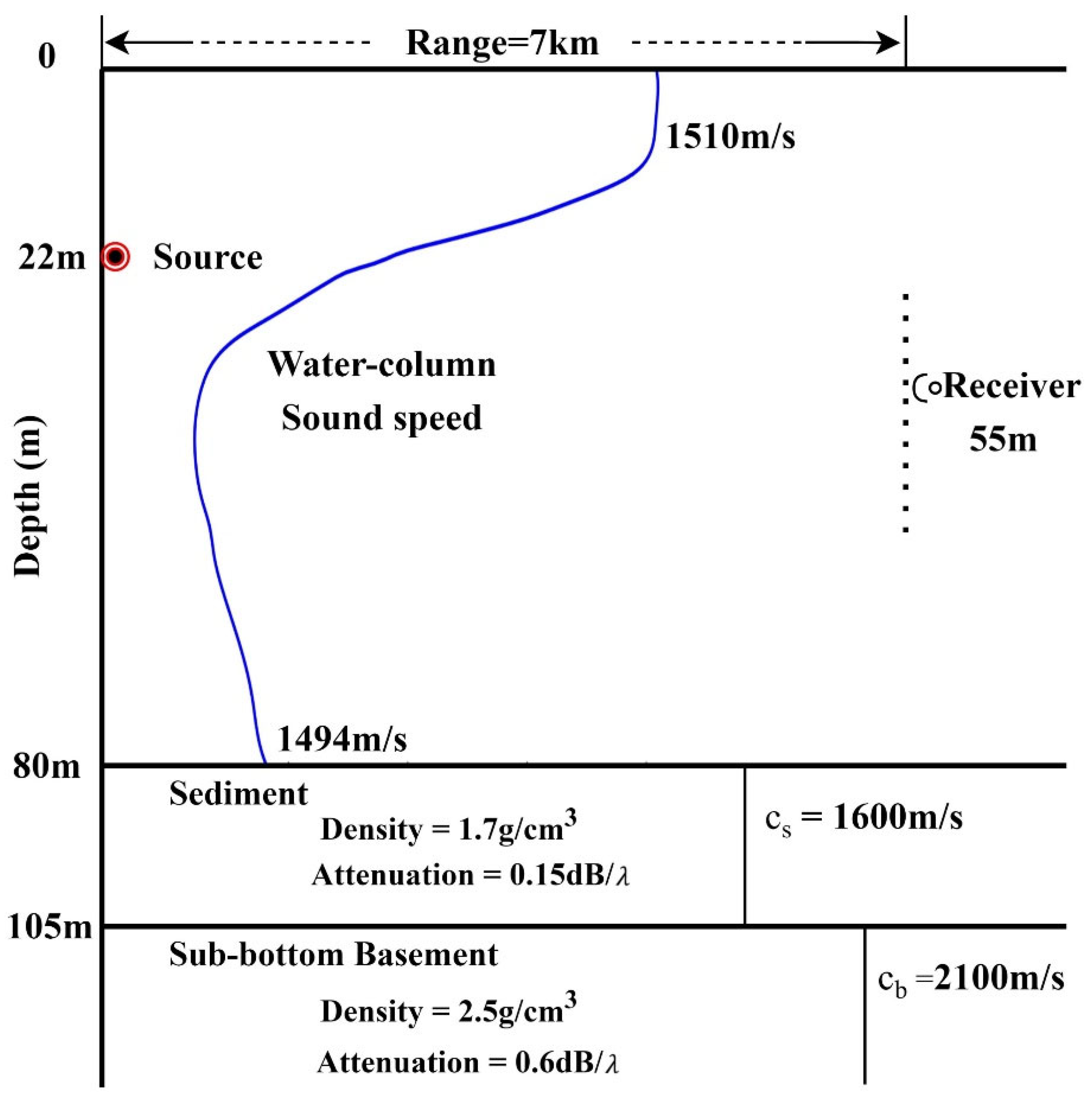
The particular way DCs and waveform matching approaches are combined in this study is guided by experience acquired from extensive numerical simulations under conditions approximating those encountered in the Shallow Water 2006 (SW06) experiment, as shown in Figure 1. In this simulation, the choice of parameterization scheme for the geoacoustic model and the configuration of environmental parameters are based on previous research findings [36] from the SW06 experiment.
Synthetic analysis of the environment is conducted using sound speed profiles [15] taken from the SW06 experiment, which shows a sediment layer on top of a deeper sub-bottom layer. The comparison is drawn utilizing the synthetic data sets computed for the two-layer geoacoustic model specified in Table 1, which parameterizes the seabed layers in terms of thickness , density , sound speed and attenuation coefficient . The sound speed and bathymetry are taken as given, and the range-independent inversion is used to estimate the seabed parameters. As evidenced in Table 1, the model priors for the inversion were set to a broad range. Hamilton’s [37] empirical relationships were employed to place lower and upper limits on sound speed (in meters per second) based on the density (in grams per cubic centimeter) of
The source pulse given by a Hanning-weighted 4-period wave is emitted at depth 22 m and recorded 7 km away at depth 55 m. As shown in Figure 2a, the received pulse consists of only one wave packet for the channel frequency response at each sampled frequency. Because the source function is well known for the simulation, no source level convolution is required. Gaussian errors were added to simulated acoustic-pressure spectra to achieve average signal-to-noise ratio (SNR) of 10 dB.
Furthermore, the inversion results of the multi-objective inversion approach are analyzed using two alternative objective functions, the L2 norm and the Wasserstein metric. The two components of Bayesian optimization are a probabilistic surrogate model and an acquisition function. In this numerical experiment, we employed a Gaussian process (GP) as the probabilistic surrogate model to facilitate the execution of MOBO. Expected improvement (EI) [26] serves as the acquisition function, which selects trials based on a heuristic aimed at maximizing improvement. There is no unique global solution, but rather a set of solutions known as the Pareto frontier in multi-objective optimization problems. The misfit residuals (as well as data-error covariance matrix) are firstly determined by attempting an optimization process in iterations of the burn-in phase. Each optimization involved ~1 103 forward calculations.
By utilizing time warping, the DCs of four lower-order normal modes can be extracted from the 50–250 Hz frequency band and used to invert for geoacoustic parameters.
The corresponding spectrogram in Figure 3c is obtained by time-frequency transformation of the time series presented in Figure 2a. From the spectrogram, it is evident that the signal energy is well contained below 150 Hz. This spectrogram with highly coupled first and second modes cannot be used for modal filtering because they are too heavily coupled. However, it can be used to assess the standard of the filtering result in a visual manner. Figure 3a demonstrates that none of the four warping modes are nearly perfectly horizontal: a sensible conclusion as the warping function is derived from an iso-velocity appropriation. The signal recovered after reverse warping plotted in Figure 2c demonstrates the reversibility of the method. As shown in Figure 3b, applying a self-customized mask to the spectrogram of the warped signal yields the spectrogram of a single warped mode. Then inverse Short-Time Fourier Transform is applied to such modes to realize modal filtering and the dispersion curve is estimated. The results show that even the modes with interleaved peak textures on the spectrogram can still be separated by the warping transform. Additionally, the unwarping transform effectively restores the original signals. These findings highlight the stability and utility of the warping transform as a method for extracting DCs. In conclusion, four modes were extracted from the data within the frequency band 50–150 Hz and applied in the dispersion inversion.
4.2. Comparison between Individual Inversions and Multi-Objective Inversions
The computational cost is a significant consideration in geoacoustic inversion due to the multiple forward calculations and the inversion algorithms. The average running times of the four methods of L2-DCs, L2-FWH, L2-MOBO and Wasserstein-MOBO, are 2750 s, 2910 s, 3620 s and 3305 s, respectively. Multi-objective frameworks have significantly higher time complexity than separated-objective frameworks. Although the Wasserstein metric formula is more complex, the computational cost of the L2-MOBO approach is higher than that of the Wasserstein-MOBO approach. This may be related to the convexity of the objective function.
Table 2 shows that the inverted Bayes estimator values (as well as standard deviation) for individual inversions using DCs are in good agreement whereas, using FWH, some parameters vary substantially. The L2-DCs method outperforms the other three techniques in terms of accurately estimating the sound speed and thickness of the sediment layer, according to Table 2. Similarly, the Wasserstein-MOBO method yields comparable results to L2-DCs in terms of sediment sound speed, demonstrating significantly lower levels of uncertainty compared to both L2-FWH and L2-MOBO approaches. However, all four methods exhibit limited effectiveness when it comes to basement sound speed. This indicates that the algorithms or characteristics employed by these approaches may not sufficiently account for the complex physical processes associated with basement layer. Assessing the NRMSE, both L2-FWH and L2-MOBO methods show similar values, approximately 7.3 × 10⁻⁵, which are notably higher than the NRMSE value of 5.67 × 10⁻⁵ obtained by the Wasserstein-MOBO method. According to Figure 4, among the observed data, posteriori replicas, and best replicas (obtained through the optimal geoacoustic parameters), the matching performance of the DCs’ inversion is particularly strong for the first three DCs. Figure 4 shows the fit of the individual inversion to the observed modal-dispersion data. This figure illustrates an impressive level of agreement between the measured DCs data and the replica data for ensemble of models taken moderately from the algorithm generations in inversion. Note that the mismatch of the fourth mode below 95 Hz is rather large, which is probably caused by the rough estimation of Airy phase, shown in Figure 3c. According to Figure 4, the robust inversion result can be attributed to the DCs’ insensitivity to the parameters, apart from sediment thickness and sound speed.
The envelope spectrum of the analog received signal shown in Figure 5a indicates that modes are highly coupled together, making modal attenuation information difficult to extract without modal filtering. The first three modes are visible in the real part of the Hilbert analytic signal, and there is no complex coupling, which is essential for geoacoustic attenuation inversion, as shown in Figure 5. The 95% credible interval of the FWH-BO inversion (gray interval in Figure 5b) widens with time, indicating that the uncertainty of FWH inversion results increases with modal order. The credible interval for first-order modal inversion results is 9.7%, while the credible intervals for second-order and third-order values are 38.6% and 37.1%, respectively. In general, within 4–6 s sampling, the objective function of FWH is well-matched, and the RMSE of the replica and observation is only 0.0108.
5. Discussion
Figure 6 depicts the distributions of likelihood functions in the posteriori probability space. Based on Figure 6, it can be seen that both misfit measures exhibit numerous local minima, but with different characteristics in terms of specific details. The distribution of the likelihood function space for DCs based on the L2 norm exhibits a convex ridge-like distribution along with the axis. Comparing Figure 6b,d, it can be concluded that the misfit function based on the Wasserstein metric significantly improves the convexity of the posterior distribution of the likelihood function obtained from MOBO inversion.
To characterize these uncertainties more generally, the posterior models are used to calculate the NRMSE for each method, as shown in Table 2. The NRMSE of Wasserstein -MOBO inversion is significantly smaller compared to that of the inversion using DCs. To help explain the results, Figure 7 and Figure 8 display marginal probability densities from Bayesian inference of estimated model parameters in MOBO inversion.
The final posterior distribution was constructed by selecting 10,000 models from the exploitation phase. The 5000 models of the posterior distribution were then ordered by likelihood and divided into three groups: the top 20%, 50%(medium), and all models. Figure 7 and Figure 8 show an example of the L2-MOBO analysis and Wasserstein-MOBO analysis, respectively. The seabed sound speed interfaces and corresponding observed data fits from the chosen models in each group, and the posterior distributions of sediment thickness, sediment density, basement density, sediment attenuation and basement attenuation for all models are also shown.
According to Figure 7, the trends of most measured and predicted data points are in accordance with each other within the estimated uncertainty. The majority of DCs show a good fit, except for the third modal Airy phase, while the FWH are not well-matched in all details. The wide distribution of basement attenuation signifies a higher degree of uncertainty and potential bias associated with the parameter. In this simulation, the modal energy for the first four modes is concentrated within 15 m of the sea floor, so the inversion is not sensitive to the basement geoacoustic parameters [21]. It is also worth noting the presence of skewness and asymmetry in the distribution of sediment thickness H. The overestimation of low-frequency estimates of the DCs can lead to such an asymmetry, which is consistent with the matching results in Figure 7c.
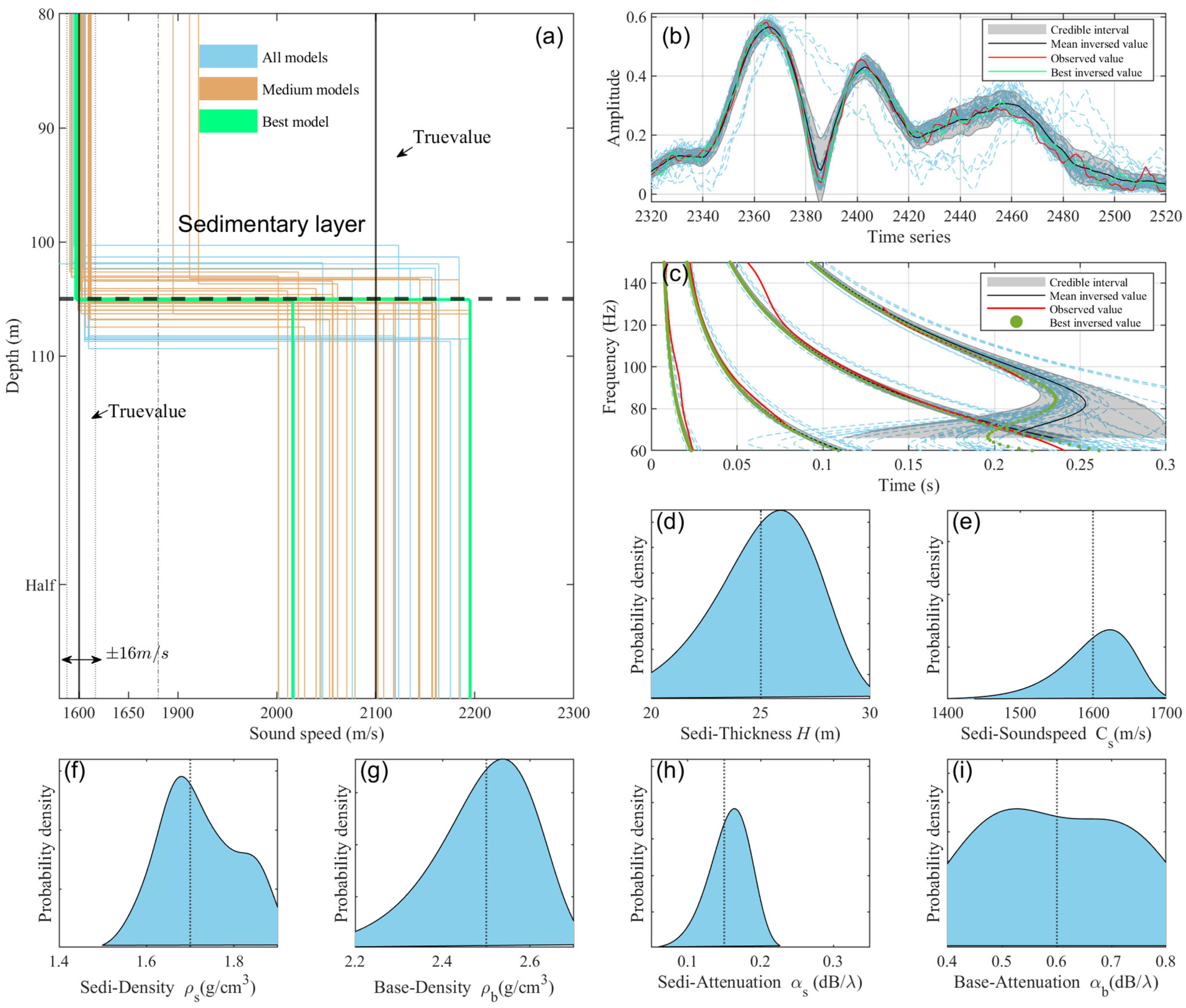
Figure 8 shows the posterior model results of the Wasserstein-MOBO analysis. By comparing the matching of FWH in Figure 7 and Figure 8, the result in L2-MOBO exhibits a wider distribution of credible intervals in the inversion of sediment sound speed . In contrast, the Wasserstein-MOBO method shows a narrower distribution of credible intervals. The bimodal distribution of basement sound speed suggests that the parameter can take on two distinct sets of values with relatively high probabilities. However, for the majority of parameters, the Wasserstein-MOBO inversion yields more accurate results, particularly for sediment sound speed, where it results in narrower marginal peak that is closer to the true value. In addition, both methods provide accurate estimates of the sediment sound speed with uncertainties significantly lower than that of the basement sound speed . The marginal distribution of basement attenuation under both metrics exhibits a bimodal pattern, indicating that the MOBO method is insensitive to this parameter.
6. Conclusions
Broadband multi-objective geoacoustic inversions using simulated data, under conditions approximating those encountered in SW06, have been performed to exhibit the advantage of the MOBO approach in reducing inversion uncertainty. It was demonstrated that, under conditions of moderate SNRs, inversion techniques employing modal-dispersion analysis and Hilbert spectral analysis of waveform data yield equivalent marginal distributions of geoacoustic parameters, including attenuation, when compared to inversions using individual DCs. Nevertheless, the adoption of the L2 norm objective function results in notable variances in the overall multidimensional posterior probability distributions, thus amplifying the uncertainty associated with the inversion process. Introducing the Wasserstein metric, however, significantly alleviates this uncertainty, leading to improved inversion outcomes.
Although MOBO, as a multi-feature inversion method, achieved more stable inversion results than individual-feature inversion methods under the same simulated conditions, it is important to note that numerical experiments did not directly consider the impact of parameterization errors when compared to realistic experiments. It is worth mentioning that 50 chains of random initial models were sampled in parallel in the simulations. This guarantees good coverage of the solution space sampling and also increases confidence in the posterior. This simulated validation reinforces the reliability and effectiveness of the MOBO method and this muti-objective approach also provides new insights and possibilities for geoacoustic inversion.
However, this current approach still requires improvement in selecting the hyperparameters for the softplus function in the Wasserstein metric and in choosing the combination of data sets. In subsequent research, validation experiments will be conducted by incorporating experiment data with different SNR conditions to assess the performance of this method, providing more convincing results for geoacoustic inversion research. Future research could also explore alternative objective functions, such as the mixed L1/Wasserstein metric [38] and the generalized L2 norm [39], to assess the suitability of this approach.
Author Contributions
Conceptualization, J.D., X.Z., P.Y. and Y.F.; methodology, J.D.; software, J.D.; validation, J.D. and X.Z.; formal analysis, J.D.; investigation, J.D.; resources, J.D. and X.Z.; data curation, J.D.; writing—original draft preparation, J.D.; writing—review and editing, J.D. and X.Z.; visualization, J.D.; supervision, X.Z. and P.Y.; project administration, X.Z.; funding acquisition, X.Z. All authors have read and agreed to the published version of the manuscript.
Funding
This research was funded by the National Natural Science Foundation of China (grant number 41775027), the National Natural Science Foundation of China (grant number 42305159) and the Natural Science Foundation of Jiangsu Province (grant number BK20231490).
Data Availability Statement
The data presented in this study are available on request from the corresponding author.
Acknowledgments
The authors gratefully acknowledge Julien Bonnel for the discussion on geoacoustic inversion using warping operators.
Conflicts of Interest
The authors declare no conflict of interest.
References
- Sun, M.; Jin, S. Multiparameter Elastic Full Waveform Inversion of Ocean Bottom Seismic Four-Component Data Based on a Modified Acoustic-Elastic Coupled Equation. Remote Sens. 2020, 12, 2816. [Google Scholar] [CrossRef]
- Zhou, J. Normal Mode Measurements and Remote Sensing of Sea-Bottom Sound Velocity and Attenuation in Shallow Water. J. Acoust. Soc. Am. 1985, 78, 1003–1009. [Google Scholar] [CrossRef]
- Oddo, P.; Falchetti, S.; Viola, S.; Pennucci, G.; Storto, A.; Borrione, I.; Giorli, G.; Cozzani, E.; Russo, A.; Tollefsen, C. Evaluation of Different Maritime Rapid Environmental Assessment Procedures with a Focus on Acoustic Performance. J. Acoust. Soc. Am. 2022, 152, 2962–2981. [Google Scholar] [CrossRef]
- Dosso, S.E. Environmental Uncertainty in Ocean Acoustic Source Localization. Inverse Probl. 2003, 19, 419–431. [Google Scholar] [CrossRef]
- Collins, M.D.; Turgut, A.; Buckingham, M.J.; Gerstoft, P.; Siderius, M. Selected Topics of the Past Thirty Years in Ocean Acoustics. J. Theor. Comp. Acout. 2022, 30, 2240001. [Google Scholar] [CrossRef]
- Chapman, N.R.; Shang, E.C. Review of Geoacoustic Inversion in Underwater Acoustics. J. Theor. Comp. Acout. 2021, 29, 2130004. [Google Scholar] [CrossRef]
- Wan, L.; Badiey, M.; Knobles, D.P. Geoacoustic Inversion Using Low Frequency Broadband Acoustic Measurements from L-Shaped Arrays in the Shallow Water 2006 Experiment. J. Acoust. Soc. Am. 2016, 140, 2358–2373. [Google Scholar] [CrossRef] [PubMed]
- Sazontov, A.G.; Malekhanov, A.I. Matched Field Signal Processing in Underwater Sound Channels (Review). Acoust. Phys. 2015, 61, 213–230. [Google Scholar] [CrossRef]
- Shi, J.; Dosso, S.E.; Sun, D.; Liu, Q. Geoacoustic Inversion of the Acoustic-Pressure Vertical Phase Gradient from a Single Vector Sensor. J. Acoust. Soc. Am. 2019, 146, 3159–3173. [Google Scholar] [CrossRef]
- Song, H.C.; Byun, G. An Overview of Array Invariant for Source-Range Estimation in Shallow Water. J. Acoust. Soc. Am. 2022, 151, 2336–2352. [Google Scholar] [CrossRef]
- Dettmer, J.; Dosso, S.E.; Holland, C.W. Full Wave-Field Reflection Coefficient Inversion. J. Acoust. Soc. Am. 2007, 122, 3327–3337. [Google Scholar] [CrossRef] [PubMed]
- Wang, Z.; Ma, Y.; Kan, G.; Liu, B.; Zhou, X.; Zhang, X. An Inversion Method for Geoacoustic Parameters in Shallow Water Based on Bottom Reflection Signals. Remote Sens. 2023, 15, 3237. [Google Scholar] [CrossRef]
- Potty, G.R.; Miller, J.H.; Lynch, J.F. Inversion for Sediment Geoacoustic Properties at the New England Bight. J. Acoust. Soc. Am. 2003, 114, 1874–1887. [Google Scholar] [CrossRef] [PubMed]
- Tan, T.W.; Godin, O.A.; Katsnelson, B.G.; Yarina, M. Passive Geoacoustic Inversion in the Mid-Atlantic Bight in the Presence of Strong Water Column Variability. J. Acoust. Soc. Am. 2020, 147, EL453–EL459. [Google Scholar] [CrossRef]
- Tan, T.W.; Godin, O.A. Passive Acoustic Characterization of Sub-Seasonal Sound Speed Variations in a Coastal Ocean. J. Acoust. Soc. Am. 2021, 150, 2717–2737. [Google Scholar] [CrossRef]
- Bonnel, J.; McNeese, A.R.; Wilson, P.S.; Dosso, S.E. Geoacoustic Inversion Using Simple Hand-Deployable Acoustic Systems. IEEE J. Ocean. Eng. 2023, 48, 592–603. [Google Scholar] [CrossRef]
- Guarino, A.L.; Smith, K.B.; Gemba, K.; Godin, O.A. Geoacoustic Inversion Using Waveform Matching as a Preliminary Step in Dispersion Curve Analysis to Assess Bottom Attenuation from a Single Vector Sensor. In Proceedings of the International Congress on Acoustics, Gyeongju, Republic of Korea, 24–28 October 2022; p. ABS-0288. [Google Scholar]
- Zhou, J.-X.; Zhang, X.-Z.; Knobles, D.P. Low-Frequency Geoacoustic Model for the Effective Properties of Sandy Seabottoms. J. Acoust. Soc. Am. 2009, 125, 2847–2866. [Google Scholar] [CrossRef]
- Bonnel, J.; Chapman, N.R. Geoacoustic Inversion in a Dispersive Waveguide Using Warping Operators. J. Acoust. Soc. Am. 2011, 130, EL101–EL107. [Google Scholar] [CrossRef]
- Bonnel, J.; Gervaise, C.; Nicolas, B.; Mars, J.I. Single-Receiver Geoacoustic Inversion Using Modal Reversal. J. Acoust. Soc. Am. 2012, 131, 119–128. [Google Scholar] [CrossRef]
- Bonnel, J.; Dosso, S.E.; Ross Chapman, N. Bayesian Geoacoustic Inversion of Single Hydrophone Light Bulb Data Using Warping Dispersion Analysis. J. Acoust. Soc. Am. 2013, 134, 120–130. [Google Scholar] [CrossRef]
- Guo, Q.; Zhang, H.; Tian, J.; Liang, L.; Shang, Z. A Nonlinear Multiparameter Prestack Seismic Inversion Method Based on Hybrid Optimization Approach. Arab. J. Geosci. 2018, 11, 48. [Google Scholar] [CrossRef]
- Zhao, X.; Huang, S. Atmospheric Duct Estimation Using Radar Sea Clutter Returns by the Adjoint Method with Regularization Technique. J. Atmos. Ocean. Technol. 2014, 31, 1250–1262. [Google Scholar] [CrossRef]
- Bonnel, J.; Thode, A.; Wright, D.; Chapman, R. Nonlinear Time-Warping Made Simple: A Step-by-Step Tutorial on Underwater Acoustic Modal Separation with a Single Hydrophone. J. Acoust. Soc. Am. 2020, 147, 1897–1926. [Google Scholar] [CrossRef]
- Rajan, S.D. Waveform Inversion for the Geoacoustic Parameters of the Ocean Bottom. J. Acoust. Soc. Am. 1992, 91, 3228–3241. [Google Scholar] [CrossRef]
- Feng, Y.; Schranner, F.S.; Winter, J.; Adams, N.A. A Multi-Objective Bayesian Optimization Environment for Systematic Design of Numerical Schemes for Compressible Flow. J. Comput. Phys. 2022, 468, 111477. [Google Scholar] [CrossRef]
- Jensen, F.B.; Kuperman, W.A.; Porter, M.B.; Schmidt, H. Normal Modes. In Computational Ocean Acoustics; Jensen, F.B., Kuperman, W.A., Porter, M.B., Schmidt, H., Eds.; Modern Acoustics and Signal Processing; Springer: New York, NY, USA, 2011; pp. 337–455. ISBN 978-1-4419-8678-8. [Google Scholar]
- Bonnel, J.; Le Touze, G.; Nicolas, B.; Mars, J.I. Physics-Based Time-Frequency Representations for Underwater Acoustics: Power Class Utilization with Waveguide-Invariant Approximation. IEEE Signal Process. Mag. 2013, 30, 120–129. [Google Scholar] [CrossRef]
- Bonnel, J.; Caporale, S.; Thode, A. Waveguide Mode Amplitude Estimation Using Warping and Phase Compensation. J. Acoust. Soc. Am. 2017, 141, 2243–2255. [Google Scholar] [CrossRef]
- Chapman, N.R. Chapter 9—Inverse Methods in Underwater Acoustics. In Applied Underwater Acoustics; Neighbors, T.H., Bradley, D., Eds.; Elsevier: Amsterdam, The Netherlands, 2017; pp. 553–585. ISBN 978-0-12-811240-3. [Google Scholar]
- Porter, M. The KRAKEN Normal Mode Program; Naval Research Laboratory: Washington, DC, USA, 2006. [Google Scholar]
- Westwood, E.K.; Tindle, C.T.; Chapman, N.R. A Normal Mode Model for Acousto-elastic Ocean Environments. J. Acoust. Soc. Am. 1996, 100, 3631–3645. [Google Scholar] [CrossRef]
- Zheng, G.; Zhu, H.; Wang, X.; Khan, S.; Li, N.; Xue, Y. Bayesian Inversion for Geoacoustic Parameters in Shallow Sea. Sensors 2020, 20, 2150. [Google Scholar] [CrossRef]
- Yang, Y.; Engquist, B.; Sun, J.; Hamfeldt, B.F. Application of Optimal Transport and the Quadratic Wasserstein Metric to Full-Waveform Inversion. Geophysics 2018, 83, R43–R62. [Google Scholar] [CrossRef]
- Engquist, B.; Froese, B.D. Application of the Wasserstein Metric to Seismic Signals. Commun. Math. Sci. 2014, 12, 979–988. [Google Scholar] [CrossRef]
- Bonnel, J.; Pecknold, S.P.; Hines, P.C.; Chapman, N.R. An Experimental Benchmark for Geoacoustic Inversion Methods. IEEE J. Ocean. Eng. 2021, 46, 261–282. [Google Scholar] [CrossRef]
- Holland, C.W.; Dosso, S.E. Hamilton’s Geoacoustic Model. J. Acoust. Soc. Am. 2022, 151, R1–R2. [Google Scholar] [CrossRef] [PubMed]
- Li, D.; Lamoureux, M.P.; Liao, W. Application of an Unbalanced Optimal Transport Distance and a Mixed L1/Wasserstein Distance to Full Waveform Inversion. Geophys. J. Int. 2022, 230, 1338–1357. [Google Scholar] [CrossRef]
- da Silva, S.L.E.F.; Karsou, A.; de Souza, A.; Capuzzo, F.; Costa, F.; Moreira, R.; Cetale, M. A Graph-Space Optimal Transport Objective Function Based on q-Statistics to Mitigate Cycle-Skipping Issues in FWI. Geophys. J. Int. 2022, 231, 1363–1385. [Google Scholar] [CrossRef]
Figure 1.
Simulated geoacoustic model and sound speed profile obtained from SW06 experiment. The source depth is 22 m, and a single receiver is placed 7.0 km away from the source at depth 55 m. Note that the graph is not to scale.
Figure 1.
Simulated geoacoustic model and sound speed profile obtained from SW06 experiment. The source depth is 22 m, and a single receiver is placed 7.0 km away from the source at depth 55 m. Note that the graph is not to scale.

Figure 2.
(Color online) Numerical signals. (a,b) show the received and corresponding warped signals, respectively. (c) The signal after warping (the continuous curves) and unwarping (the red circles). Keep in mind that the time axes of the two subfigures are not equivalent.
Figure 2.
(Color online) Numerical signals. (a,b) show the received and corresponding warped signals, respectively. (c) The signal after warping (the continuous curves) and unwarping (the red circles). Keep in mind that the time axes of the two subfigures are not equivalent.

Figure 3.
(Color online) (a) Spectrogram of the warped signal. The white polygon shows the region of the TF mask applied to filter mode 3. (b) The frequency spectrum of the warped signal for the frequency band 0–50 Hz, and the embedded graph is warped mode 3. (c) Spectrogram of the received signal. White dotted lines represent the theoretical DCs for the first four modes. The estimated DCs are also displayed as red curves upon the time-frequency spectrogram (panel (c)).

Figure 4.
(Color online) Data fit achieved in inversions of DCs. Comparison between the observed modal-dispersion data (red solid lines) and the posteriori ensembles (blue dashed lines) obtained from DCs-BO inversion. The green dotted line represents the best model and the gray region is a 95% credible interval from the Bayesian sampling.

Figure 5.
(Color online) (a) The upper envelope (red line) and lower envelope (orange line) of the observed data. (b) Data fits achieved in FWH inversion. Comparison between the observed FWH data (blue solid lines) and the posteriori ensembles (purple dashed lines) obtained from FWH-BO inversion. The green solid line represents the best model and the gray region is the 95% credible interval from the Bayesian sampling.

Figure 6.
The posterior distribution of likelihood function in MOBO inversions, with black solid points representing the true values. (a,b) Likelihood distributions of DCs based on (a) L2 term and (c) Wasserstein metric. (c,d) Likelihood distributions of FWH based on (c) L2 term and (d) Wasserstein metric.

Figure 7.
Posteriori models based on L2-MOBO and corresponding data fits for (b) FWH and (c) DCs, along with marginal distributions of (d) sediment thickness, (e) sediment sound speed, (f) sediment density, (g) basement density, (h) sediment attenuation and (i) basement attenuation. (a) Models of sound velocity and sediment depth. The results are represented with different colors, indicating the probability of the models, from the best 20%, 50% (medium) and all. Black vertical lines mark the actual sound speed values in the sediment and basement. The horizontal dashed line and the patch show the true value and distribution interval of sediment depth, respectively. The black solid lines, red solid lines and blue dashed lines in (b,c) indicate the average inversion values, observed values, and misfits under the posterior, respectively. The grouping of the best and full models and the colors are consistent with (a). The grey uncertainty intervals in (b,c) represent the range of values that contains the mean of the data, with a 95% credible interval. Black vertical dashed lines in (d–i) represent the true value of parameters.

Figure 8.
Posteriori models based on Wasserstein-MOBO and corresponding data fits for (b) FWH and (c) DCs, along with marginal distributions of (d) sediment thickness, (e) sediment sound speed, (f) sediment density, (g) basement density, (h) sediment attenuation and (i) basement attenuation. (a) Models of sound velocity and sediment depth. The results are represented with different colors, indicating the probability of the models, from the best 20%, 50% (medium) and all. Black vertical lines mark the actual sound speed values in the sediment and basement. The horizontal dashed line and the patch show the true value and distribution interval of sediment depth, respectively. The black solid lines, red solid lines and blue dashed lines in (b,c) indicate the average inversion values, observed values, and misfits under the posterior, respectively. The grouping of the best and full models and the colors are consistent with (a). The grey uncertainty intervals in (b,c) represent the range of values that contains the mean of the data, with a 95% credible interval. Black vertical dashed lines in (d–i) represent the true value of parameters.


Table 1.
Inversion parameters and uniform prior bounds.
| Parameter | Units | True Values | Prior Bounds |
|---|---|---|---|
| Layer thickness 1 | m | 25.0 | [20, 30] |
| Sediment sound speed | 1600.0 | [1440, 2500] | |
| Sediment density | 1.7 | [1.3, 2.4] | |
| Sediment attenuation | 0.15 | [0.05, 0.5] | |
| Basement sound speed | 2100.0 | [1440, 2500] | |
| Basement density | 2.5 | [1.3, 2.4] | |
| Basement attenuation | 0.6 | [0.05, 0.7] | |
| Time shift | — | [−1.0, 2.0] |
1 Except for the basement half space.
Table 2.
Summary of individual BO inversion (DCs & FWH) and MOBO inversion results. A mean of the posterior distribution, called a Bayes estimator, with 95% credible interval uncertainties is also given. The rightmost column gives the normalized root-mean-square error (NRMSE) of this inversion results.
| Parameter | NRMSE | |||||||
|---|---|---|---|---|---|---|---|---|
| L2-DCs | 24.5 (±2.9) | 1601.0 (±5.8) | 1.65 (±0.11) | 2260.0 (±119.7) | 2.58 (±0.16) | —— | —— | —— |
| L2-FWH | 29.7 (±4.2) | 1619.5 (±13.6) | 1.89 (±0.15) | 2091.0 (±99.4) | 2.45 (±0.13) | 0.220 (±0.025) | 0.405 (±0.158) | 7.35 × 10⁻⁵ |
| L2-MOBO | 26.3 (±2.4) | 1635.5 (±39.5) | 1.75 (±0.08) | 2077.5 (±122.0) | 2.55 (±0.12) | 0.160 (±0.025) | 0.628 (±0.125) | 7.32 × 10⁻⁵ |
| Wasserstein-MOBO | 27.1 (±4.3) | 1605.5 (±6.5) | 1.75 (±0.08) | 2136.0 (±70.0) | 2.54 (±0.11) | 0.170 (±0.015) | 0.604 (±0.125) | 5.67 × 10⁻⁵ |
Disclaimer/Publisher’s Note: The statements, opinions and data contained in all publications are solely those of the individual author(s) and contributor(s) and not of MDPI and/or the editor(s). MDPI and/or the editor(s) disclaim responsibility for any injury to people or property resulting from any ideas, methods, instructions or products referred to in the content. |
© 2023 by the authors. Licensee MDPI, Basel, Switzerland. This article is an open access article distributed under the terms and conditions of the Creative Commons Attribution (CC BY) license (https://creativecommons.org/licenses/by/4.0/).
Share and Cite
MDPI and ACS Style
Ding, J.; Zhao, X.; Yang, P.; Fu, Y. A Multi-Objective Geoacoustic Inversion of Modal-Dispersion and Waveform Envelope Data Based on Wasserstein Metric. Remote Sens. 2023, 15, 4893. https://doi.org/10.3390/rs15194893
AMA Style
Ding J, Zhao X, Yang P, Fu Y. A Multi-Objective Geoacoustic Inversion of Modal-Dispersion and Waveform Envelope Data Based on Wasserstein Metric. Remote Sensing. 2023; 15(19):4893. https://doi.org/10.3390/rs15194893
Chicago/Turabian StyleDing, Jiaqi, Xiaofeng Zhao, Pinglv Yang, and Yapeng Fu. 2023. "A Multi-Objective Geoacoustic Inversion of Modal-Dispersion and Waveform Envelope Data Based on Wasserstein Metric" Remote Sensing 15, no. 19: 4893. https://doi.org/10.3390/rs15194893
Note that from the first issue of 2016, this journal uses article numbers instead of page numbers. See further details here.