Eigenvector Constraint-Based Method for Eliminating Dead Zone in Magnetic Target Localization

Abstract

Magnetic target localization using the magnetic gradient tensor (MGT) plays a significant role in underwater localization. However, this method inherently has a localization dead zone, which presents challenges for real-world applications. This paper delves into the root cause of this dead zone, identifying the non-invertibility of the MGT when the magnetic moment vector is orthogonal to the position vector from the target to the observation point. To tackle this issue, a method based on the eigenvector constraints is proposed. By constructing an objective function with eigenvector constraints and leveraging the property that its gradient at the observation point is zero, we derive an equivalent expression for the inverse of MGT that always holds and further develop a dead-zone-free localization method. To validate the robustness and efficacy of the proposed localization method, a comparative analysis with other methods is conducted. Simulation results in a 10 m × 10 m area under Gaussian noise demonstrate the proposed method’s capability to eliminate the dead zone and achieve an average localization error of 0.032 m. Experimental results further demonstrate that the proposed method eliminates the localization dead zone and exhibits greater robustness than the dominant method in the normal region. In summation, this paper provides an effective method for eliminating localization dead zone, offering a more stable and reliable method for magnetic target localization in practice.

1. Introduction

Ferromagnetic materials in the geomagnetic field are magnetized and generate an induced magnetic field, referred to as the magnetic anomaly. Ferromagnetic materials can be located by measuring the magnetic anomaly and processing the data accordingly. Magnetic target localization technology has significant practical applications in various fields. For instance, in underwater magnetic localization, it aids in mapping the undersea terrain and identifying buried magnetic objects [1,2]. It is also employed in detecting unexploded ordnance, where it helps identify and safely remove potential threats [3,4]. In medical interventions, this technology is applied in steering magnetic catheters and tracking wireless biomedical capsule [5,6]. The dominant approach adopted in magnetic target localization is the analytical method, which leverages the relationship between the magnetic field vector, the magnetic gradient tensor (MGT), and the tensor invariant to derive the localization formula. These formulas, which are straightforward and easy to solve, generally meet the requirements for real-time operation and accuracy across diverse application scenarios.

Magnetic target localization based on MGT has been extensively studied. The various localization methods can be divided into three categories: the single-point tensor positioning (SPTP), the two-point tensor positioning (TPTP), and the scalar triangulation and ranging (STAR). In the SPTP method, Wynn’s pioneering use of MGT for magnetic target detection showed the apparent advantages and potential of MGT [7]. Following this, Frahm et al. [8] enhanced the Wynn method by applying MGT in the point-by-point localization. Since then, numerous scholars and researchers have explored magnetic target localization to enhance the localization accuracy of the SPTP method. Nara et al. [9] derived a closed-form linear equation for localizing a magnetic dipole. The magnetic target is located by multiplying the inverse matrix of MGT with the magnetic anomaly of the target. Yin et al. [10] developed a MGT system approximating the first-order and second-order spatial gradients of magnetic field components with finite differences. Sui et al. [11] constructed expressions for the second-order and third-order gradient tensors and proposed a method for extracting these tensors from a uniaxial magnetic field sensor. Wang et al. [12] proposed a stability optimization algorithm based on the improved central difference method. These methods have less localization error. However, the high order quantity is significantly affected by the measurement noise and the geomagnetic field noise.

To address the issue that the SPTP method will be affected by the geomagnetic field noise, some researchers adopted the TPTP method. Xu et al. [13] proposed a linear localization method based on the two-point magnetic gradient full tensor. However, this method requires the two observation points to be closely spaced to avoid errors. Liu et al. [14] proposed a new TPTP method based on the magnetic moment constraints and used the PSO algorithm to optimize the penalty coefficient and localization error. However, due to the iterative calculations required by the PSO algorithm, the real-time performance of the localization method is compromised. Liu et al. [15] established a two-point MGT localization model and derived the localization equations. Although localization can be obtained accurately by solving these equations, there are some localization dead zones.

Through the exploration of MGT, some researchers discovered that tensor invariant might provide novel localization ideas. Wiegert et al. [16,17,18] proposed a new magnetic dipole localization method called STAR, which constructs equations based on spatial variations of the MGT invariant. This independence from the geomagnetic field is a significant advantage. However, the STAR method assumes that the tensor invariant is a perfect sphere, leading to asphericity errors in the localization. Wang et al. [19] adopted an iterative algorithm to compensate for the asphericity errors of the STAR method and reduced the relative localization error. Though the methods previously discussed are effective, they necessitate the use of multiple gradiometers for measurements, which limits their widespread application.

The three methods, SPTP, TPTP, and STAR, have their own advantages and disadvantages. However, the majority of these methods involve the computation of the inverse matrix of MGT. If MGT is non-invertible, these localization methods will fail, leading to localization dead zones. To tackle this issue, some scholars have proposed localization methods with no dead zones. Nara et al. [20] improved the localization method by using the Moore–Penrose generalized inverse matrix instead of the inverse matrix. However, the determination of the singularity of the matrix can be easily affected by measurement noise. Higuchi et al. [21] adopted truncated singular value decomposition approach to propose a new localization equation. Yin et al. [22] proposed a new close-form formula for magnetic dipole localization. However, these two methods are derived from the basis of the SPTP method and are not applicable to TPTP and STAR. Pei et al. [23] adopted a regularization method to address the non-invertibility issue of MGT, but the localization error remains significant.

In summary, all three methods encounter dead zone issues due to the non-invertibility of MGT. To address this shortcoming, a localization method based on eigenvector constraints with the dead zone free is proposed. Additionally, this method is can be used to eliminate dead zones in other localization methods. A regularization term based on the eigenvector constraints is introduced into the objective function which is constructed with Euler’s equation. As the objective function gradient at the observation point is zero, the equivalent expression of the inverse MGT and the localization equation without a dead zone are derived. Through the algebraic operation, the localization equation will not fail at arbitrary points in space, thereby eliminating the localization dead zone. Simulation and experimental results demonstrate that the localization equation is more accurate and robust.

2. Localization Dead Zone Analysis

When the detection distance significantly surpasses the size of the magnetic target, it is feasible to simplify the magnetic target into a magnetic dipole model. The spatial Cartesian coordinate system is established to define the magnetic field and MGT, taking the magnetic target as the origin. A schematic diagram is depicted in Figure 1. In this system, according to the Biot–Savart Law, the magnetic field at the observation point is given by:

$$\mathit{B}=\frac{{\mu }_0}{4\pi }\frac{3\left(\mathit{M}·{\mathit{n}}_{\mathit{r}}\right){\mathit{n}}_{\mathit{r}}-\mathit{M}}{r^3}$$

(1)

where $\mathit{B}$ represents the magnetic field intensity, ${\mu }_0$ represents the vacuum permeability, $\mathit{M}$ represents the magnetic moment of the magnetic target, and $\mathit{r}$ is the position vector extending from the magnetic target to the observation point. The unit vector of $\mathit{r}$ is represented by ${\mathit{n}}_{\mathit{r}}$, and $\mathit{r}$ signifies the length of $\mathit{r}$.

Assume that the magnetic field at the adjacent observation point, $\mathit{r}+d\mathit{r}$, is ${\mathit{B}}^{\prime }$. The magnetic field difference between these two positions is:

$$\begin{array}{c}{\mathit{B}}^{\prime }-\mathit{B}=\frac{{\mu }_0}{4\pi }\left[3\left(\mathit{M}·{\mathit{n}}_{\mathit{r}}\right){\mathit{n}}_{\mathit{r}}-\mathit{M}\right]\left[\frac{1}{{(r+dr)}^3}-\frac{1}{r^3}\right]\\ =\frac{{\mu }_0}{4\pi }\left[3\left(\mathit{M}·{\mathit{n}}_{\mathit{r}}\right){\mathit{n}}_{\mathit{r}}-\mathit{M}\right]\frac{\partial }{\partial r}\left(\frac{1}{r^3}\right)dr=-\frac{3}{r}\mathit{B}dr\end{array}$$

(2)

Alternatively, the magnetic field intensity difference between the two points can also be given as:

$${\mathit{B}}^{\prime }-\mathit{B}=\left[\begin{array}{ccc}\frac{\partial B_x}{\partial x}& \frac{\partial B_x}{\partial y}& \frac{\partial B_x}{\partial z}\\ \frac{\partial B_y}{\partial x}& \frac{\partial B_y}{\partial y}& \frac{\partial B_y}{\partial z}\\ \frac{\partial B_z}{\partial x}& \frac{\partial B_z}{\partial v}& \frac{\partial B_z}{\partial z}\end{array}\right] {\mathit{n}}_{\mathit{r}}dr=G{\mathit{n}}_{\mathit{r}}dr$$

(3)

where $\mathit{G}$ denotes MGT. Considering both Equations (2) and (3), the localization formula based on MGT can be expressed as:

$$\mathit{r}=-3G^{-1}\mathit{B}$$

(4)

This formula is the localization formula of the Nara method. It shows that if MGT and the magnetic field are known, the position can be determined. This formula is straightforward and involves only the inversion and multiplication of third-order matrices. However, it should be noted that MGT is not always invertible, and the method have a localization dead zone. To fully understand the applicability of the algorithm, the analytical expression of the MGT matrix is given by:

$$G_{ij}=-\frac{3{\mu }_0}{4\pi }\frac{(\mathit{M}·\mathit{r})\left(5r_i{r}_j-r^2{\delta }_{ij}\right)-r^2\left(r_i{M}_j+r_j{M}_i\right)}{r^7}$$

(5)

where ${\delta }_{ij}$ is the Kronecker delta and i, j represent x, y, and z in the spatial Cartesian coordinate system.

To simplify the computation, the Cartesian coordinate system is redefined, which is shown in the Figure 2.

In this spatial Cartesian coordinate system, the magnetic target becomes the origin. The x-axis aligns with the direction of the position vector, and the magnetic moment vector lies in the x-y plane. $\theta$ represents the angle between the position vector and the magnetic moment vector. The position vector is expressed as $\mathit{r}=(\mathit{r},0,0)$, and the magnetic moment vector as $\mathit{M}=(\mathit{M}\cos \theta ,\mathit{M}\sin \theta ,0)$. The MGT at the observation point is then expressed as:

$$G=\frac{3{\mu }_{0}M}{4\pi r^4}\left[\begin{array}{ccc}-2cos\theta & \sin \theta & 0\\ \sin \theta & \cos \theta & 0\\ 0& 0& \cos \theta \end{array}\right]$$

(6)

When $\theta$ equals ${90}^{\circ }$, the matrix G becomes non-invertible, causing the localization method to fail. In space, all points satisfying $\theta ={90}^{\circ }$ will form a plane, representing the theoretical dead zone of the localization algorithm. Moreover, points near the dead zone may also cause the determinant of MGT to approach zero due to calculational precision and processor capabilities, thereby expanding the dead zone. To address this issue, it becomes necessary to identify a formula independent of the computation’s angle. The relationship between the eigenvalues and the eigenvectors is used to propose the method for eliminating dead zone, which is detailed in the next section. The expressions of the eigenvalues and the eigenvectors are given by:

$$\left\{\begin{array}{c}{\lambda }_1=\frac{3{\mu }_{0}M}{8\pi r^4}\left(-\cos \theta +\sqrt{5{\cos }^2\theta +4}\right)\hfill \\ {\lambda }_2=\frac{3{\mu }_{0}M}{4\pi r^4}\cos \theta \hfill \\ {\lambda }_3=\frac{3{\mu }_{0}M}{8\pi r^4}\left(-\cos \theta -\sqrt{5{\cos }^2\theta +4}\right)\hfill \end{array}\right.$$

(7)

$$\left\{\begin{array}{c}{\mathit{v}}_1={(2\sin \theta ,3\cos \theta -\sqrt{5{\cos }^2\theta +4},0)}^T\hfill \\ {\mathit{v}}_2={(0,0,1)}^T\hfill \\ {\mathit{v}}_3={(2\sin \theta ,3\cos \theta +\sqrt{5{\cos }^2\theta +4},0)}^T\hfill \end{array}\right.$$

(8)

where ${\lambda }_i$ ($i=1,2,3$) denote the eigenvalues of G, and ${\mathit{v}}_i$ ($i=1,2,3$) represent the corresponding eigenvectors. It is important to note that the three eigenvalues satisfy the relationship ${\lambda }_1\ge {\lambda }_2\ge {\lambda }_3$. Furthermore, in terms of absolute values, $|{\lambda }_1| \ge |{\lambda }_2|$ and $|{\lambda }_3| \ge |{\lambda }_2|$. With these established relationships, ${\lambda }_2$ can be determined by sorting the eigenvalues and calculate the corresponding eigenvector $v_2$. It is worth mentioning that $v_2$ satisfies the equation:

$${\mathit{v}}_2^T\mathit{r}=0$$

(9)

It is worth noting that while Equation (9) was derived in the coordinate system presented in Figure 2, it remains valid in any coordinate system. The tensor is a quantity that remains invariant with respect to changes in the coordinate system. Once the magnetic moment intensity and direction of the magnetic target and the relative position of the observation point to the magnetic target are determined, MGT is a fixed value. This can also be verified from Equation (6). Therefore, to simplify the calculation process, the spatial Cartesian coordinate system shown in Figure 2 is chosen. This coordinate system has three characteristics: firstly, it takes the magnetic target as the origin; secondly, the observation point is in the positive direction of the x-axis; and thirdly, the magnetic moment vector lies within the x–y plane. In this system, the expression for the second eigenvector of MGT can be conveniently derived, further proving that this eigenvector is orthogonal to the plane formed by the position vector and the magnetic moment vector. This conclusion is universally true and remains invariant regardless of changes in the coordinate system.

3. Eigenvector-Constrained Method for Dead Zone Elimination

Based on the analysis of the preceding section, the Nara method is straightforward for magnetic target localization. However, when the position vector and the magnetic moment vector are orthogonal, the analytical solution is unstable, leading to a localization dead zone algorithmically. Therefore, the Tikhonov regularization technique is employed to address the issues of unstable solutions in this paper. The objective function can be constructed as follows:

$$f=\min {\parallel G\mathit{r}+3\mathit{B}\parallel }_2^2$$

(10)

In the system shown in Figure 2, the Hessian matrix, denoted as H, of f is:

$$H=\frac{9{\mu }_0^2{M}^2}{8{\pi }^2{r}^8}\left[\begin{array}{ccc}3{\cos }^2\theta +1& \sin \theta \cos \theta & 0\\ \sin \theta \cos \theta & 1& 0\\ 0& 0& {\cos }^2\theta \end{array}\right]$$

(11)

The eigenvalues of matrix H can be computed as:

$$\left\{\begin{array}{c}{\lambda }_{H1}={\cos }^2\theta \hfill \\ {\lambda }_{H2}=\frac{3{\cos }^2\theta }{2}-\frac{\cos \theta \sqrt{5{\cos }^2\theta +4}}{2}+1\hfill \\ {\lambda }_{H3}=\frac{3{\cos }^2\theta }{2}+\frac{\cos \theta \sqrt{5{\cos }^2\theta +4}}{2}+1\hfill \end{array}\right.$$

(12)

Through algebraic operations, it show that the eigenvalue ${\lambda }_{H1}$ is non-negative, and the remaining two eigenvalues are positive. Hence, the Hessian matrix is positive semidefinite, indicating that the objective function is convex.

$\mathit{r}$, denoting the position vector, satisfies Equations (2) and (3). Thus, the value of the objective function f is zero. Otherwise, the value of f exceeds zero. As such, the objective function reaches the unique global minimum solely at the observation point, where the gradient is zero. This conclusion implies that the position vector satisfies the following relationship:

$$\frac{\partial f}{\partial \mathit{r}}=2G^{T}G\mathit{r}+6G^T\mathit{B}=0$$

(13)

This relationship derives the formula for the position vector:

$$\mathit{r}=-3{\left(G^{T}G\right)}^{-1}{G}^T\mathit{B}$$

(14)

However, G becomes singular when the position vector and the magnetic moment vector are orthogonal. Consequently, the solution of Equation (14) is unstable. The issue that the matrix singularity leads to the unstable solution has been addressed in numerous previous studies, which have demonstrated that introducing a Tikhonov regularization term to the objective function can stabilize the solution [24]. Based on Equation (9), the new objective function is constructed as follows:

$$f=\min \left({\parallel G\mathit{r}+3\mathit{B}\parallel }_2^2+\alpha {∥{\mathit{v}}_2^T\mathit{r}∥}_2^2\right)$$

(15)

where $\alpha$ is the penalty coefficient used to adjust the intensity of the regularization term. This objective function will still reach a unique global minimum at the location of the magnetic target; thereby, the formula of the position vector is yielded:

$$\mathit{r}=-3{\left(G^2+\alpha {\mathit{v}}_2{\mathit{v}}_2^T\right)}^{-1}GB$$

(16)

To guarantee a stable solution for Equation (16), it is crucial to validate whether the term $G^2+\alpha {\mathit{v}}_2{\mathit{v}}_2^T$ is singular. In the system in Figure 2, the determinant of the term $G^2+\alpha {\mathit{v}}_2{\mathit{v}}_2^T$ is given by:

$$|G^2+\alpha {\mathit{v}}_2{\mathit{v}}_2^T|={\left(\frac{3{\mu }_{0}M}{4\pi r^4}\right)}^6{\left({\sin }^2\theta -2\right)}^2\left({\cos }^2\theta +\alpha \right)$$

(17)

Clearly, if $\alpha$ is positive, the determinant of $G^2+\alpha {\mathit{v}}_2{\mathit{v}}_2^T$ remains positive, ensuring the stable solution for Equation (16). This proposed method effectively eliminates the localization dead zone in magnetic target localization based on MGT.

Furthermore, as the $\alpha$ approaches 0, the expression ${\left(G^2+\alpha {\mathit{v}}_2{\mathit{v}}_2^T\right)}^{-1}G$ can be effectively represented as the expression $G^{-1}$. Specifically, both expression ${\left(G^2+\alpha {\mathit{v}}_2{\mathit{v}}_2^T\right)}^{-1}G$ and expression $G^{-1}$ are third-order matrices. They only differ in the ninth element, which are $\frac{\cos \theta }{{\cos }^2\theta +\alpha }$ and $\frac{1}{\cos \theta }$, respectively. Therefore, when $\alpha$ is sufficiently small, ${\left(G^2+\alpha {\mathit{v}}_2{\mathit{v}}_2^T\right)}^{-1}G$ can be used in place of $G^{-1}$ for calculations, effectively eliminating the dead zone in the magnetic target localization without affecting localization accuracy.

As regards selecting the penalty coefficient, the L-curve method a commonly used method in Tikhonov regularization. This method graphically determines the optimal penalty coefficient by plotting the trade-off between the solution norm ${∥{\mathit{v}}_2^T\mathit{r}∥}_2^2$ and the residual norm ${\parallel G\mathit{r}+3\mathit{B}\parallel }_2^2$. As the penalty coefficient changes, the regularized solutions are computed, and the norms are plotted, forming an L-shaped curve. The corner of this curve signifies a balance between data misfit and solution complexity, representing the optimal penalty coefficient. This approach efficiently finds the optimal penalty coefficient.

4. Numerical Simulations

4.1. Magnetic Target Localization Dead Zone

To verify that the condition for the formation of the localization dead zone is the orthogonality between the position vector and the magnetic moment vector, simulations were conducted on the widely-used Nara method [9]. In these simulations, a magnetic dipole was situated at the origin of a spatial Cartesian coordinate system. In this system, the magnetic moment vector of the dipole was defined as $(-327,-425,132)$ Am${}^2$. The localization results were tested at multiple observation points within a rectangular region situated 3 m above the origin. The coordinates of the four vertices of this rectangle are (−5, −5, 3) m, (−5, 5, 3) m, (5, −5, 3) m, and (5, 5, 3) m. The intervals between observation points in both the x and y directions are 0.02 m. According to Equation (4), to achieve magnetic target localization, it is necessary to measure the magnetic field intensity and MGT. Therefore, the magnetic sensor array structure shown in Figure 3 was employed to measure these two quantities.

In this array, each dark square represents a three-axis magnetic sensor, which measures the magnetic field component at its position. The formulas for the magnetic field intensity and the MGT are given by:

$$\mathit{B}=\frac{{\mathit{B}}_1+{\mathit{B}}_2+{\mathit{B}}_3+{\mathit{B}}_4}{4}$$

(18)

$$\mathit{G}=\left|\begin{array}{ccc}{\mathit{B}}_{1x}-{\mathit{B}}_{3x}\hfill & {\mathit{B}}_{2x}-{\mathit{B}}_{4x}\hfill & {\mathit{B}}_{1z}-{\mathit{B}}_{3z}\\ {\mathit{B}}_{2x}-{\mathit{B}}_{4x}\hfill & {\mathit{B}}_{2y}-{\mathit{B}}_{4y}\hfill & {\mathit{B}}_{2z}-{\mathit{B}}_{4z}\\ {\mathit{B}}_{1z}-{\mathit{B}}_{3z}\hfill & {\mathit{B}}_{2z}-{\mathit{B}}_{4z}\hfill & {\mathit{B}}_{4y}+{\mathit{B}}_{3x}-{\mathit{B}}_{2y}-{\mathit{B}}_{1x}\end{array}\right|$$

(19)

The total localization error, denoted as $\epsilon$, is used to reflect the localization performance at each point. The formula for the total localization error is as follows:

$$\epsilon =\sqrt{{\epsilon }_x^2+{\epsilon }_y^2+{\epsilon }_z^2}$$

(20)

where ${\epsilon }_x$ denotes the localization error in x-axis, ${\epsilon }_y$ denotes the localization error in y-axis, ${\epsilon }_z$ denotes the localization error in z-axis,

Figure 4 illustrates the distribution of the total localization error across the simulation region. The maximum observed localization error is substantial, reaching up to 11,284.5 m. To emphasize the characteristics of the error distribution, all error results are transformed using a base-10 logarithm. In the figure, most of the region is shaded in blue, which signifies that the localization error in these areas is less than 1 m. A prominent line is visible in the image, representing locations with a significantly larger localization error. This highlights limitations in the Nara method, suggesting that it may not provide reliable results at these specific points.

All observation points with a localization error greater than 2 m were extracted. Subsequently, the angles between the magnetic moment vectors and position vectors at these points were computed. A histogram was then created for these angles, followed by a normal distribution fitting, with the results displayed in the Figure 5.

Through an integrated analysis of observation points within the dead zone, angles corresponding to the position vectors and the magnetic moment vectors were computed. A statistical representation of these angles was visualized using a histogram, which was subsequently fitted with a normal distribution curve in red. When the number of bins is set to 9, the fit to the normal distribution is improved. At this setting, the mean of the normal distribution is $90.6^{\circ }$, with a standard deviation of $1.3^{\circ }$. This result illustrates the orthogonality relationship between the position vectors and the magnetic moment vectors within the dead zone. It provides compelling evidence that the formation of the localization dead zone is attributed to this orthogonal relationship.

4.2. Optimization of the Penalty Coefficient

The penalty coefficient plays a pivotal role in regularized solutions by balancing the trade-off between the fit to the data and the complexity of the solution. Its value determines the extent to which the regularization term influences the solution. The L-curve method is a common graphical tool utilized to identify the optimal penalty coefficient. By plotting the solution norm against the residuals norm, an L-shaped curve emerges. The corner of this curve typically signifies the optimal penalty coefficient, striking a balance between solution smoothness and data fidelity.

To determine the optimal penalty coefficient for the proposed method, all observation points within the simulation plane from the previous chapter were utilized. Based on preliminary analysis, the range for the penalty coefficient was set between ${10}^{-16}$ and 10 with 100 logarithmically spaced values. Each value was then incorporated into the proposed method, localizing all observation points, and the average solution norm ${∥{\mathit{v}}_2^T\mathit{r}∥}_2^2$ and the average residual norm ${\parallel G\mathit{r}+3\mathit{B}\parallel }_2^2$ were computed. Ultimately, plotting the average solution norm against the average residual norm for these varying coefficients yielded Figure 6.

From the Figure 6, it is evident that the curve exhibits a distinct L-shape. Moreover, the elbow of the L-curve is positioned where the residual norm ${\parallel G\mathit{r}+3\mathit{B}\parallel }_2^2$ is about $3.71\times {10}^{-9}$ and the solution norm ${∥{\mathit{v}}_2^T\mathit{r}∥}_2^2$ is about $3.40\times {10}^{-15}$. At this point, a balance between the solution norm and the residual norm is achieved. Hence, the optimal penalty coefficient is 0.2154.

4.3. Proposed Magnetic Target Localization Method

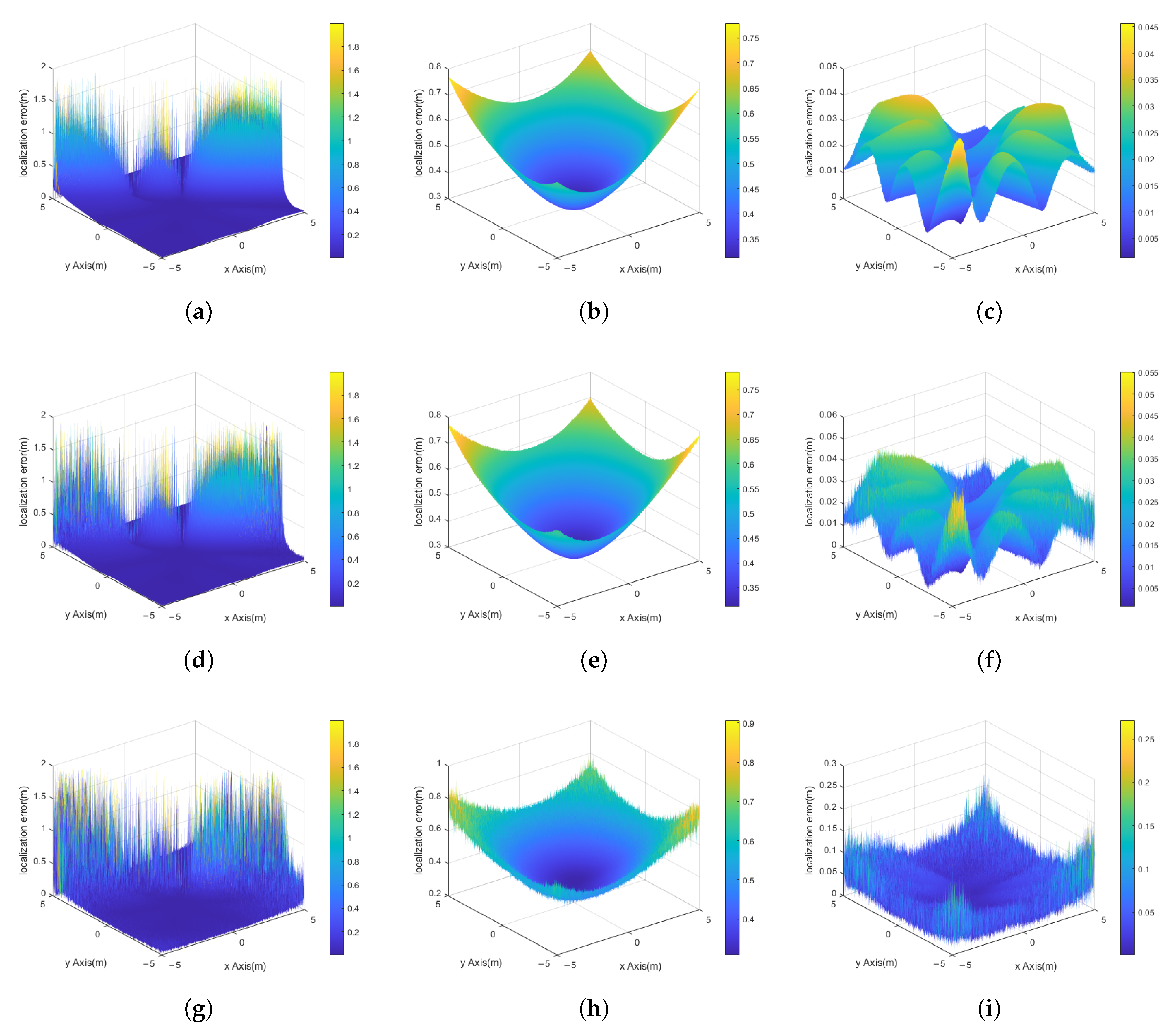
To validate the proposed localization method, a series of numerical simulations were conducted. The magnetic dipole was positioned at the origin of a spatial Cartesian coordinate system, with its magnetic moment vector set to $(-327,-425,132)$ Am${}^2$ within this system. Observation points, arranged with a grid spacing of 0.02 m, were situated on a 10 m × 10 m plane elevated at a height of 3 m. To assess the robustness, the Gaussian noise was introduced into the two measurements of the magnetic field vector and the MGT. To analyze the effectiveness and robustness of the proposed method, the Nara method and the Pei method were chosen for comparison. the Nara method is currently the widely adopted method, while the Pei method addresses the dead zone issue using the Tikhonov regularization technique.

Figure 7 illustrates the distribution of localization errors for the three methods under different geomagnetic field noise levels.

Table 1. Statistical results of localization errors of three methods under different magnetic field noises.

Methods	Geomagnetic Field Noise	Mean	Std
Nara	0.01 nT	0.0449 m	0.0858 m
	0.1 nT	0.0452 m	0.0860 m
	1 nT	0.0682 m	0.1110 m
Pei	0.01 nT	0.4824 m	0.0969 m
	0.1 nT	0.4824 m	0.0969 m
	1 nT	0.4828 m	0.0983 m
Proposed	0.01 nT	0.0197 m	0.0081 m
	0.1 nT	0.0198 m	0.0081 m
	1 nT	0.0304 m	0.0192 m

displays the mean and standard deviation of localization errors for the three methods under different geomagnetic field noise levels. Due to the presence of localization dead zones, the Nara method exhibits instances of very large localization errors. For ease of comparison, data with a localization error exceeding 1 m is not displayed and is excluded from statistical analysis.

While the Nara method has apparent localization dead zones, statistical data indicate that its localization error within normal regions is relatively small. The Pei method effectively eliminates localization error, but its error diverges at a faster rate as distance increases, leading to larger mean and standard deviation values for the localization error. The proposed method not only effectively eradicates localization dead zones but also exhibits a slower divergence rate of localization error with increasing distance. Under a geomagnetic field noise with a standard deviation of 1 nT, the localization error at the farthest point does not exceed 0.25 m.

From the perspective of robustness, under the noise levels of 0.1 nT and 0.01 nT, the distribution of localization error for the proposed method remains consistent. This indicates that the localization error at this point mainly stems from the localization method itself. At a noise level of 1 nT, the localization error is predominantly influenced by geomagnetic noise interference. Nevertheless, the localization error is still lower than that of the other two methods.

Figure 8 displays the distribution of localization errors for the three methods under varying levels of magnetic gradient noises.

Table 2. Statistical results of localization errors of three methods under different magnetic gradient noises.

Methods	Magnetic Gradient Noise	Mean	Std
Nara	0.01 nT	0.0449 m	0.0858 m
	0.1 nT	0.0471 m	0.0881 m
	1 nT	0.0957 m	0.1375 m
Pei	0.01 nT	0.4824 m	0.0969 m
	0.1 nT	0.4824 m	0.0970 m
	1 nT	0.4851 m	0.1039 m
Proposed	0.01 nT	0.0197 m	0.0081 m
	0.1 nT	0.0205 m	0.0090 m
	1 nT	0.0523 m	0.0498 m

presents the corresponding mean and standard deviation of the localization error. Both Figure 8 and Table 2 similarly confirm that the proposed method not only effectively eliminates localization dead zones but also possesses stronger robustness. However, it is distinct that magnetic gradient noise of the same intensity has a greater impact on localization than magnetic field noise. Under 0.01 nT and 0.1 nT noise levels, this observation is not as pronounced because the localization error induced by the noise is lesser than the inherent error of the localization method itself. At 1 nT magnetic field noise, both the mean and standard deviation of the localization error are noticeably lower than those under 1 nT magnetic gradient noise. This underscores that the proposed localization method is more sensitive to magnetic gradient noise. Nonetheless, the localization performance of the proposed method still outperforms the other two methods.

5. Experiments

5.1. Localization Error in the Localization Dead Zone

To validate the efficacy of the proposed method, a field experiment was performed in an area characterized by a relatively stable magnetic field. As shown in Figure 9, the MGT measurement system comprises three main components: a magnetic target, a planar cross-shaped MGT measurement array, and a data processor. The magnetic target is a neodymium magnet, emitting a magnetic field intensity of approximately 2500 Gauss. The direction of the magnetic moment is also illustrated in Figure 9. The planar cross-shaped MGT measurement array consists of four triaxial fluxgate magnetometers secured to a cross-shaped bracket. This bracket stands 0.45 m high, with each magnetometer positioned 0.25 m from the bracket’s center. The data processor’s role is to capture the magnetic data and implement the localization method.

Several measures have been taken to minimize interference from magnetic fields not generated by magnetic targets. The cross-shaped bracket for the magnetic sensor array is made of resin material to ensure that it does not produce any additional magnetic fields. The test environment was carefully chosen to be an open area, ensuring a relatively stable ambient magnetic field. All magnetic objects were distanced from the measurement area to mitigate magnetic interference. To further eliminate interference from the environmental magnetic field, the background magnetic field was measured at the same point before and after the magnetic target’s placement. The magnetic gradient of the magnetic target was then determined by subtracting the magnetic data obtained from these two conditions.

In this experiment, the setup was designed to ensure that the position vector and the magnetic moment vector were orthogonal, as illustrated in Figure 9. The projection of the center of the cross-shaped MGT measurement array onto the ground served as the origin, establishing a Cartesian coordinate system. The measurement line, extending 2.4 m along the y-axis, had 12 test points (excluding the origin) placed at intervals of 0.2 m and marked by the red circle in Figure 9. The positions of these test points were calculated using both the Nara method and the proposed method in this study for comparison.

The results of different localization methods are displayed in Figure 10, while Figure 11 presents the corresponding localization errors. In Figure 10, the actual test points and the localization points calculated by the three methods are indicated using different markers. Since the test points are all located within the dead zone, the localization points from the Nara method are significantly distant from the test points, while those from the Pei method and the proposed method are close to the test points. Figure 11 provides a more detailed depiction of the localization errors of these three methods. For comparison, the y axis is represented in logarithmic scale. The localization error of the proposed method is noticeably superior to the Pei method when the magnetic target is close to the MGT measurement device, but at a slightly greater distance, the localization errors of the two methods are almost the same level.

5.2. Localization Error in Normal Region

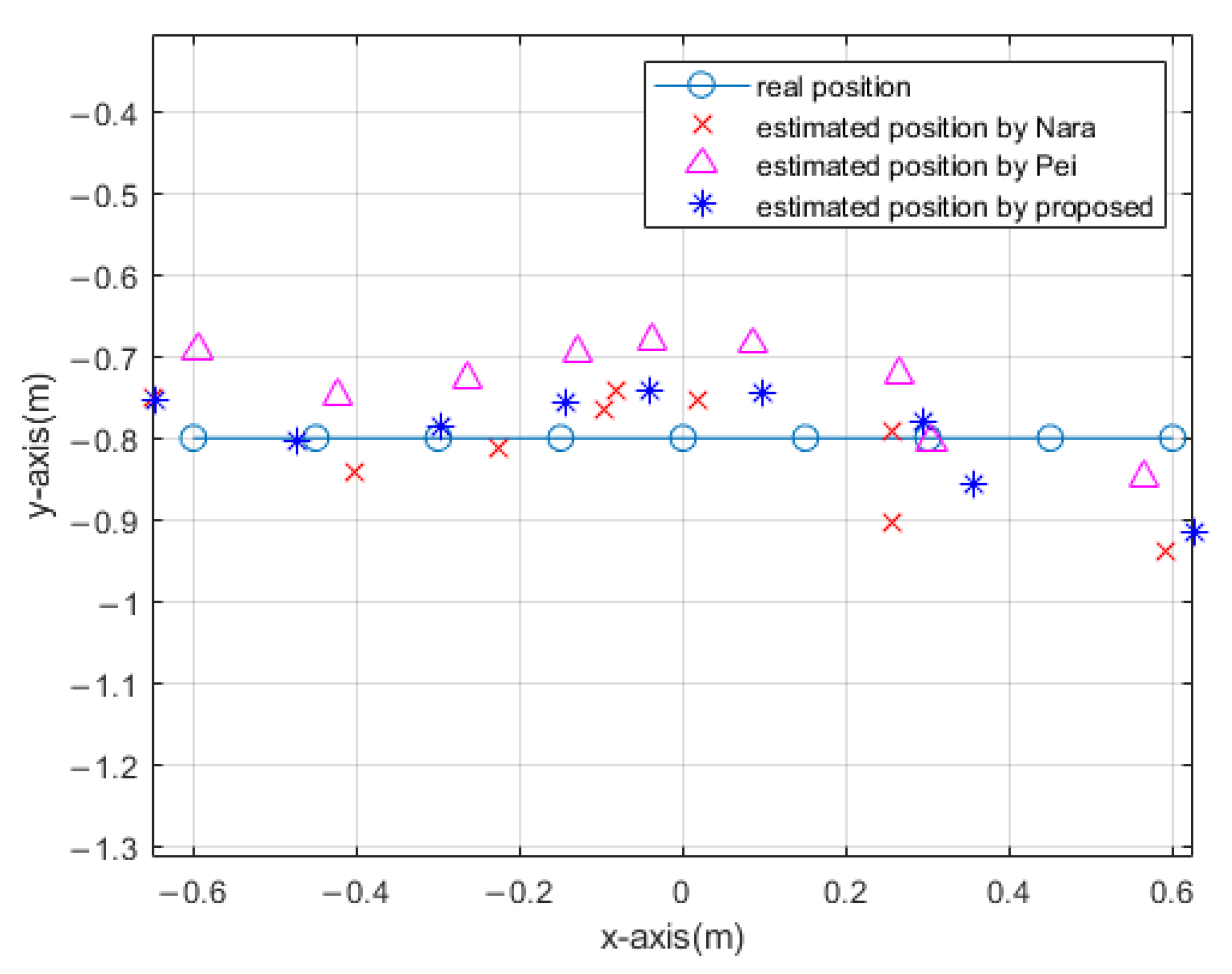
To assess the precision of the proposed localization method under more diverse conditions, a line was established to ensure that the position vector and the magnetic moment vector were not orthogonal. The coordinates of this measurement line’s endpoints were set at $(-0.6,1,0)$ m and $(0.6,1,0)$ m, respectively. A total of 9 test points were set along this line, spaced at 0.15 m intervals.

In Figure 12, the test points and the localization points from the three methods are marked using different indicators. The localization points from all three methods are primarily close to the test points, indicating that they all possess certain localization capabilities. For a more detailed comparison of the localization errors, Figure 13 uses three distinct markers to represent the localization errors for each measurement point according to the three methods. It is evident that the localization error of the proposed method is significantly smaller than the other two methods, especially in positions close to the MGT measurement device.

From the above two experiments, it can be discerned that both the proposed method and the Pei method effectively eliminate localization dead zones. However, the proposed method demonstrates higher localization accuracy and robustness than the Pei method, making it more suitable for practical applications.

6. Conclusions

Magnetic target localization, a critical task with implications across various fields, relies heavily on MGT-based methods. However, this paper reveals a significant limitation of magnetic target localization, specifically its failure in the region where the position vector and the magnetic target’s magnetic moment vector are orthogonal, resulting in a singular MGT and an unstable solution. To address this issue, a eigenvector constraint-based magnetic target localization method is proposed. This method circumvents the singularity of MGT by introducing the regularization term, which is constrained by the eigenvector into the objective function for localization. The localization formula is derived from this objective function based on the property that the gradient of the objective function at the observation point is zero. This novel method ensures that the matrix’s determinant consistently exceeds zero, thereby eliminating the localization dead zone. The proposed method’s robustness is demonstrated through simulations and experiments. The Nara method and the Pei method are chosen for comparison. The Nara method is a widely adopted localization technique, yet it has localization dead zones. The Pei method effectively eliminates these dead zones. Simulations and experiments both confirm that the proposed method not only effectively removes localization dead zones but also exhibits higher localization accuracy and robustness than the Pei method, making it more suitable for practical applications. While the proposed method still inherits the limitations of the SPTP approach and is not suitable for areas with dramatic magnetic field variations, it provides a more reliable magnetic target localization technique for regions with relatively stable magnetic fields, such as underwater environments.

References

- Alimi, R.; Fisher, E.; Nahir, K. In Situ Underwater Localization of Magnetic Sensors Using Natural Computing Algorithms. Sensors 2023, 23, 1797. [Google Scholar] [CrossRef] [PubMed]
- Huang, X.; Wang, Y.; Ma, J.; Wu, J.; Li, J.; Zhang, Y.; Feng, H. A localization method for subsea pipeline based on active magnetization. Meas. Sci. Technol. 2023, 34, 025012. [Google Scholar] [CrossRef]
- Seidel, M.; Frey, T.; Greinert, J. Underwater UXO detection using magnetometry on hovering AUVs. J. Field Robot. 2023, 40, 848–861. [Google Scholar] [CrossRef]
- Wang, L.; Zhang, S.; Chen, S.; Luo, C. Underground Target Localization Based on Improved Magnetic Gradient Tensor with Towed Transient Electromagnetic Sensor Array. IEEE Access 2022, 10, 25025–25033. [Google Scholar] [CrossRef]
- Fischer, C.; Quirin, T.; Chautems, C.; Boehler, Q.; Pascal, J.; Nelson, B.J. Gradiometer-Based Magnetic Localization for Medical Tools. IEEE Trans. Magn. 2023, 59, 1–5. [Google Scholar] [CrossRef]
- Umay, I.; Fidan, B. Adaptive Wireless Biomedical Capsule Tracking Based on Magnetic Sensing. Int. J. Wirel. Inf. Netw. 2017, 24, 189–199. [Google Scholar] [CrossRef]
- Wynn, W. Dipole tracking with a gradiometer. In Naval Ship Research and Development Laboratory Informal Report; NSRDL/PC: Bethesda, MD, USA, 1972; p. 3493. [Google Scholar]
- Frahm, C.P. Inversion of the magnetic field. In NCSL Informal Report; NCSL: Panama, FL, USA, 1972; pp. 72–135. [Google Scholar]
- Nara, T.; Suzuki, S.; Ando, S. A closed-form formula for magnetic dipole localization by measurement of its magnetic field and spatial gradients. IEEE Trans. Magn. 2006, 42, 3291–3293. [Google Scholar] [CrossRef]
- Gang, Y.; Yingtang, Z.; Hongbo, F.; Zhining, L. Magnetic dipole localization based on magnetic gradient tensor data at a single point. J. Appl. Remote Sens. 2014, 8, 083596. [Google Scholar] [CrossRef]
- Sui, Y.; Leslie, K.; Clark, D. Multiple-Order Magnetic Gradient Tensors for Localization of a Magnetic Dipole. IEEE Magn. Lett. 2017, 8, 1–5. [Google Scholar] [CrossRef]
- Wang, B.; Ren, G.; Li, Z.; Li, Q. The stability optimization algorithm of second-order magnetic gradient tensor. AIP Adv. 2021, 11, 075322. [Google Scholar] [CrossRef]
- Xu, L.; Gu, H.; Chang, M.; Fang, L.; Lin, P.; Lin, C. Magnetic Target Linear Location Method Using Two-Point Gradient Full Tensor. IEEE Trans. Instrum. Meas. 2021, 70, 1–8. [Google Scholar] [CrossRef]
- Liu, H.; Wang, X.; Zhao, C.; Ge, J.; Dong, H.; Liu, Z. Magnetic Dipole Two-Point Tensor Positioning Based on Magnetic Moment Constraints. IEEE Trans. Instrum. Meas. 2021, 70, 1–10. [Google Scholar] [CrossRef]
- Liu, G.; Zhang, Y.; Wang, C.; Li, Q.; Li, F.; Liu, W. A New Magnetic Target Localization Method Based on Two-Point Magnetic Gradient Tensor. Remote Sens. 2022, 14, 6088. [Google Scholar] [CrossRef]
- Wiegert, R.; Oeschger, J.; Tuovila, E. Demonstration of a novel man-portable magnetic STAR technology for real time localization of unexploded ordnance. In Proceedings of the OCEANS 2007, Vancouver, BC, Canada, 29 September–4 October 2007; pp. 795–801. [Google Scholar]
- Wiegert, R.; Lee, K.; Oeschger, J. Improved magnetic STAR methods for real-time, point-by-point localization of unexploded ordnance and buried mines. In Proceedings of the OCEANS 2008, Quebec City, QC, Canada, 15–18 September 2008; pp. 1–7. [Google Scholar]
- Wiegert, R. Magnetic STAR technology for real-time localization and classification of unexploded ordnance and buried mines. In Proceedings of the Detection and Sensing of Mines, Explosive Objects, and Obscured Targets XIV, Orlando, FL, USA, 13–17 April 2009; Volume 7303, pp. 514–522. [Google Scholar]
- Wang, C.; Zhang, X.; Qu, X.; Pan, X.; Fang, G.; Chen, L. A Modified Magnetic Gradient Contraction Based Method for Ferromagnetic Target Localization. Sensors 2016, 16, 2168. [Google Scholar] [CrossRef] [PubMed]
- Nara, T.; Ito, W. Moore-Penrose generalized inverse of the gradient tensor in Euler’s equation for locating a magnetic dipole. J. Appl. Phys. 2014, 115, 17E504. [Google Scholar] [CrossRef]
- Higuchi, Y.; Nara, T.; Ando, S. A Truncated Singular Value Decomposition approach for locating a magnetic dipole with Euler’s equation. Int. J. Appl. Electromagn. Mech. 2016, 52, 67–72. [Google Scholar] [CrossRef]
- Yin, G.; Zhang, L.; Jiang, H.; Wei, Z.; Xie, Y. A closed-form formula for magnetic dipole localization by measurement of its magnetic field vector and magnetic gradient tensor. J. Magn. Magn. Mater. 2020, 499, 166274. [Google Scholar] [CrossRef]
- Pei, Y.; Yeo, H. Magnetic gradiometer inversion for underwater magnetic object parameters. In Proceedings of the OCEANS 2006—Asia Pacific, Singapore, 16–19 May 2006; pp. 1–6. [Google Scholar]
- Mu, Y.; Zhang, X.; Xie, W. Calibration of Magnetometer Arrays in Magnetic Field Gradients. IEEE Magn. Lett. 2019, 10, 1–5. [Google Scholar] [CrossRef]
Figure 1.
Schematic diagram of the magnetic target localization.
Figure 2.
Schematic diagram of the magnetic target localization.The magnetic target is set as the origin of coordinates. The x-axis forwards coincides with the direction of the position vector. The magnetic moment vector is in the x-y plane.
Figure 3.
Array structure of the magnetic gradient sensor.
Figure 4.
Distribution of the localization error of the Nara method in plane.
Figure 5.
Histogram of the angular distribution between the position vector and magnetic moment vector at observation points within the dead zone.
Figure 6.
The L-curve corresponding to all observation points within the simulation plane.
Figure 7.
Localization errors of the three methods under different magnetic field noises. (a) Nara method under 0.01 nT geomagnetic field noise. (b) Pei method under 0.01 nT geomagnetic field noise. (c) Proposed method under 0.01 nT geomagnetic field noise. (d) Nara method under 0.1 nT geomagnetic field noise. (e) Pei method under 0.1 nT geomagnetic field noise. (f) Proposed method under 0.1 nT geomagnetic field noise. (g) Nara method under 1 nT geomagnetic field noise. (h) Pei method under 1 nT geomagnetic field noise. (i) Proposed method under 1 nT geomagnetic field noise.
Figure 8.
Localization errors of the three methods under different magnetic gradient noises. (a) Nara method under 0.01 nT magnetic gradient noise. (b) Pei method under 0.01 nT magnetic gradient noise. (c) Proposed method under 0.01 nT magnetic gradient noise. (d) Nara method under 0.1 nT magnetic gradient noise. (e) Pei method under 0.1 nT magnetic gradient noise. (f) Proposed method under 0.1 nT magnetic gradient noise. (g) Nara method under 1 nT magnetic gradient noise. (h) Pei method under 1 nT magnetic gradient noise. (i) Proposed method under 1 nT magnetic gradient noise.
Figure 9.
Measurement system and experiment setup.
Figure 10.
Comparison of the localization results of three methods in the localization dead zone.
Figure 11.
Comparison of the localization errors of three methods in the localization dead zone.
Figure 12.
Comparison of the localization results of three methods in the normal region.
Figure 13.
Comparison of the localization errors of three methods in the normal region.