
Simultaneous Vehicle Localization and Roadside Tree Inventory Using Integrated LiDAR-Inertial-GNSS System

1
School of Economics and Management, Changsha University, 98 Hongshan Road, Changsha 410022, China
2
CRRC Zhuzhou Institute Co., Ltd., 169 Shidai Road, Zhuzhou 412001, China
*
Author to whom correspondence should be addressed.
Remote Sens. 2023, 15(20), 5057; https://doi.org/10.3390/rs15205057
Submission received: 20 June 2023
/
Revised: 15 September 2023
/
Accepted: 17 September 2023
/
Published: 21 October 2023
(This article belongs to the Special Issue Laser Scanning for Quantifying Sustainable Forest and Agriculture Management)
Abstract
:Autonomous driving systems rely on a comprehensive understanding of the surrounding environment, and trees, as important roadside features, have a significant impact on vehicle positioning and safety analysis. Existing methods use mobile LiDAR systems (MLS) to collect environmental information and automatically generate tree inventories based on dense point clouds, providing accurate geometric parameters. However, the use of MLS systems requires expensive survey-grade laser scanners and high-precision GNSS/IMU systems, which limits their large-scale deployment and results in poor real-time performance. Although LiDAR-based simultaneous localization and mapping (SLAM) techniques have been widely applied in the navigation field, to the best of my knowledge, there has been no research conducted on simultaneous real-time localization and roadside tree inventory. This paper proposes an innovative approach that uses LiDAR technology to achieve vehicle positioning and a roadside tree inventory. Firstly, a front-end odometry based on an error-state Kalman filter (ESKF) and a back-end optimization framework based on factor graphs are employed. The updated poses from the back-end are used for establishing point-to-plane residual constraints for the front-end in the local map. Secondly, a two-stage approach is adopted to minimize global mapping errors, refining accumulated mapping errors through GNSS-assisted registration to enhance system robustness. Additionally, a method is proposed for creating a tree inventory that extracts line features from real-time LiDAR point cloud data and projects them onto a global map, providing an initial estimation of possible tree locations for further tree detection. This method uses shared feature extraction results and data pre-processing results from SLAM to reduce the computational load of simultaneous vehicle positioning and roadside tree inventory. Compared to methods that directly search for trees in the global map, this approach benefits from fast perception of the initial tree position, meeting real-time requirements. Finally, our system is extensively evaluated on real datasets covering various road scenarios, including urban and suburban areas. The evaluation metrics are divided into two parts: the positioning accuracy of the vehicle during operation and the detection accuracy of trees. The results demonstrate centimeter-level positioning accuracy and real-time automatic creation of a roadside tree inventory.
1. Introduction
Trees play a significant role in urban, interurban, and suburban road environments by enhancing the natural landscape, mitigating erosion, and improving air quality [1]. However, they also present challenges for autonomous driving systems as they can interfere with satellite positioning signals and obstruct sensor visibility, leading to decreased localization accuracy and potential missed or false detections. Moreover, even relatively small trees with diameters as little as 10.2 cm (4 inches) can pose safety risks, with a considerable number of fatal accidents involving fixed obstacles being attributed to trees [2]. Hence, it is crucial to develop an effective method for real-time localization, accurate 3D mapping, and identification and classification of roadside trees to enhance driving safety.
Traditional ground surveying techniques are time-consuming, cumbersome, and expensive. Therefore, remote sensing data such as aerial imagery or light detection and ranging (LiDAR) point clouds are valuable resources for creating tree inventories [3]. Mobile laser scanning (MLS) systems have gained prominence in road environment modeling due to their ability to safely and efficiently acquire accurate 3D information [4]. These systems generate dense point clouds by collecting coordinates of 3D points using laser pulses at a rate exceeding one million points per second. The proven capabilities of MLS systems have led to their widespread use in extracting information about the road environment, including trees, traffic signs, and other features [5,6]. However, MLS systems require high-precision GNSS/IMU measurements and survey-grade laser scanners. While they achieve high-precision 3D mapping, the associated costs hinder their large-scale deployment, making widespread applications challenging. Moreover, MLS systems exhibit lower mapping and perception efficiency, posing difficulties in meeting the real-time requirements of autonomous driving.
Simultaneous Localization and Mapping (SLAM) technology, as it continues to mature, holds promise for vehicle positioning and real-time tree inventory creation. However, there is currently a lack of methods that achieve simultaneous vehicle positioning and tree inventory creation. The primary technical challenges can be summarized as follows:
- (1)
- Long-distance tree canopies, buildings and overpasses obstruct GNSS signals, significantly reducing the accuracy of satellite navigation. Inertial Navigation Systems rely on Inertial Measurement Units (IMUs) for vehicle positioning, which can accumulate errors over time.
- (2)
- Running SLAM algorithms and tree extraction algorithms separately incurs a high computational resource cost. Existing SLAM feature extraction algorithms and tree feature extraction algorithms differ significantly, making it challenging to adopt a unified algorithm for simultaneous vehicle positioning and real-time tree inventory creation.
- (3)
- In regions with complex road conditions, fast tree detection algorithms that use shared SLAM feature information are prone to false positives due to environmental interference.
Motivated by tree inventory construction and SLAM algorithms, this paper proposes an accurate and robust vehicle positioning and tree inventory creation system that tightly integrates multi-modal sensor information. Our design offers the following contributions:
- (1)
- We introduce a positioning and mapping scheme suitable for long-distance occlusion scenarios. This scheme presents a front-end odometry based on an error-state kalman filter (ESKF) and a back-end optimization framework based on factor graphs. The updated poses from the back-end are used for establishing point-to-plane residual constraints for the front-end in the local map.
- (3)
- We adopt a two-stage approach to minimize global mapping errors, refining accumulated mapping errors through GNSS-assisted registration.
- (3)
- In this paper, we propose an innovative approach that uses shared feature extraction results and data preprocessing results from SLAM to create a tree inventory. With this method, we are able to reduce the computational cost of the system while simultaneously achieving vehicle positioning and tree detection.
- (4)
- Additionally, we introduce a method that uses azimuth angle feature information to further mitigate false positives.
- (5)
- The system is extensively evaluated in urban and suburban areas. The evaluation results demonstrate the accuracy and robustness of our system, which can effectively handle positioning and tree inventory creation tasks in various scenarios.
The remaining sections of this paper are organized as follows. Section 2 reviews related work. Section 3 presents the specific algorithms for pose estimation, mapping, and tree inventory generation used in our system. The experimental results are presented in Section 4. Finally, Section 5 summarizes the paper and provides an outlook on future research directions.
2. Related Work
Methods for creating tree inventories using MLS point clouds can be classified into manual and automated approaches. However, manual methods are time-consuming and labor-intensive. To overcome these limitations, recent research has primarily focused on developing automated methods to optimize the cost and time involved in tree inventory creation. Over the past decade, several automated methods have been developed to extract trees from laser point clouds, and they have found extensive applications in urban road planning, 3D tree modeling, tree monitoring, and structural feature quantification [7,8,9,10,11]. The individual tree segmentation from point cloud data has also received significant attention, such as capturing tree height, trunk diameter, breast diameter, and other attributes from dense point cloud information [12,13,14,15,16], as well as 3D object detection based on point cloud data [17,18]. Additionally, studies incorporating image sensors to add RGB information have also received considerable attention. For example, integrating panoramic images with MLS point clouds and adding color information from images to point clouds during segmentation as an action criterion for tree identification [19]. Similar methods include integrating multispectral image information with MLS point clouds for tree identification [20]. Most existing methods can effectively segment and extract trees [19,20,21,22]. However, these methods that rely on MLS systems require expensive high-precision GNSS/IMU positioning and survey-grade laser scanners, which limit their large-scale deployment. Moreover, the real-time performance of automatically identifying and delineating trees based on high-precision point cloud data (PCD) is low.
Lidar, with its resistance to lighting variations and precise distance measurement, has been widely used not only for object perception but also in navigation tasks [23]. Lidar sensors are becoming increasingly common in various robotic applications, such as autonomous vehicles [24,25], drones [26,27], and more. Lu et al. first transformed SLAM pose estimation into a least squares optimization problem. They linearized the nonlinear objective function using Taylor expansion and solved it using gradient descent, Gauss-Newton, or Levenberg-Marquardt methods [28]. The most classic 3D Lidar SLAM algorithm, Lidar Odometry and Mapping in Real-time (LOAM), extracts corner and planar points from each frame based on curvature and constructs feature lines based on corner points and feature planes based on planar points. By performing point cloud registration and solving the pose using a least squares method, LOAM ensures both accurate positioning and good mapping results through the use of low-frequency mapping and high-frequency localization. However, this method lacks a loop closure detection module [29]. Shan et al. made improvements to LOAM by first performing point cloud clustering and segmentation, successfully separating ground points from other points. Based on the clustering approach, unreliable point clouds were filtered out, improving the quality of feature points. They also proposed a two-step optimization method to accelerate pose estimation and convergence speed. Additionally, they introduced a loop closure detection method based on Euclidean distance to eliminate cumulative errors. This method is more efficient than LOAM and is better suited for deployment in autonomous driving systems while also surpassing LOAM in terms of system completeness [30]. Chen et al. proposed a surface-based mapping method that uses 3D point clouds combined with semantic information to improve mapping quality. Furthermore, data association is performed on objects with semantic labels, establishing a constraint relationship with geometric information to solve the pose, thereby improving mapping quality [31]. However, this method has poor real-time performance. In 2021, Wang et al. proposed a novel SLAM solution that uses both geometric and intensity information from Lidar point clouds. They designed a frontend odometry estimation based on intensity information and a backend optimization based on intensity. Their method outperforms SLAM approaches that solely rely on geometric information [32]. Ye et al. applied the Vins-Mono concept to Lidar SLAM by proposing a tightly coupled fusion method that integrates Lidar and IMU. The high-frequency data from the IMU is used for Lidar point cloud calibration through integration, and a rotation constraint method is introduced to estimate the rotation extrinsics between the IMU and Lidar. This method significantly improves accuracy compared to single Lidar positioning [33]. Lin et al. introduced a novel Lidar-Inertial-Visual sensor fusion framework called R3LIVE. It uses measurements from Lidar, inertial, and visual sensors for robust and accurate state estimation. The framework also incorporates data from visual-inertial sensors and renders map textures [34]. Wang et al. proposed a real-time, accurate, and robust positioning and mapping using Lidar SLAM. Their framework tightly couples a non-repeating scanning Lidar with IMU, wheel odometry, and GNSS for position estimation and synchronized global map generation [35]. Although current Lidar-based SLAM algorithms have demonstrated sufficient accuracy and robustness in many scenarios, they still face challenges in degraded and large-scale environments. Furthermore, the feature extraction algorithms in the aforementioned SLAM methods do not consider the requirements of tree detection and identification, making it difficult to simultaneously achieve vehicle positioning and tree inventory creation.
3. Materials and Methods
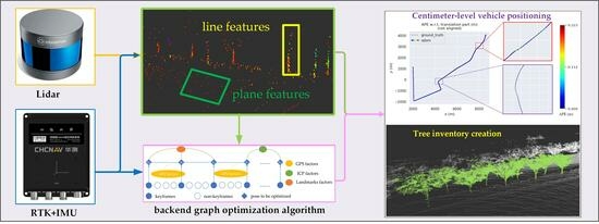
This paper presents a multi-sensor fusion solution aiming to achieve simultaneous vehicle localization and roadside tree inventory generation. The proposed solution is designed to operate reliably in challenging scenarios such as long-distance tree occlusion of satellite signals and unfavorable lighting conditions. Common options for selecting positioning, mapping, and target perception sensors include GNSS, IMU, LiDAR, and cameras. However, cameras are susceptible to lighting effects, and GNSS+IMU accumulates significant errors in long-distance occlusion scenarios. Therefore, this study primarily adopts LiDAR and integrated navigation units as the main sensors. The workflow of the system is illustrated in Figure 1.
In order to reduce the computational load of the algorithm, the proposed system first performs the extraction of edge feature points and planar feature points from the point cloud data collected by LiDAR. Subsequently, the data of these feature points is combined with the measurement data from the navigation unit to perform processes such as motion compensation and distortion removal on the feature point cloud. The motion-compensated and distortion-removed feature points are then used separately in the tree detection module and the ESKF module. The tree detection module clusters and detects trunk features, and it sends the attribute information of tree feature points to the global map to enhance the tree attribute information of the feature points. The ESKF module uses the feature points and the local map to construct a residual equation and updates the pose state with IMU preintegration. If the error state converges, the position is output; otherwise, the iteration continues. Then, based on the position output by the ESKF module, the feature points are updated and added to the global map, and the odometry position is passed to the back-end optimization module. The back-end optimization module further refines the pose of keyframes using information such as RTK and landmarks before sending it to the global map. Finally, in the global map, the orientation information of the tree feature points is used to further filter false positives of tree crowns.
3.1. Feature Extraction
3.1.1. Candidate Point Calculation
LiDAR perceives the surrounding environmental information and forms a three-dimensional point cloud. A single frame of point cloud often contains tens of thousands to hundreds of thousands of points. Using all of them for calculations would greatly consume computational resources and fail to meet real-time requirements. In reality, as shown in Figure 2, there are a large number of feature point clouds in space, such as plane points and line points. By extracting this type of point cloud, the number of points used in the calculation process can be significantly reduced, saving computation time [29,30].
Existing algorithms for calculating feature points, such as LOAM and Lego-LOAM, calculate the spatial distance between neighboring points in the same line of laser points to obtain the line curvature of that point. The line curvature is used as the criterion for classifying feature points. This method can effectively calculate plane points and line points. However, it is not suitable for tree detection, and the feature extraction becomes unstable when the incidence angle and distance of the laser change. For example, existing SLAM feature extraction methods are prone to filtering out dense tree leaves as invalid feature points, leading to the loss of points in the subsequent tree crown based on feature points. For instance, when the laser is incident at a suitable angle and distance on the tree leaves, some of the laser point cloud is reflected by the surface leaves, and a considerable portion passes through the surface leaves and is reflected back by the leaves or branches behind. In this case, corner points can be extracted well. When the incident distance is relatively close and the tree leaves are dense, multiple points reflected by the surface leaves may appear consecutively on the same beam. The calculated line curvature will be significantly reduced, and it may even be misjudged as plane points.
In this paper, an adaptive spatial geometry candidate feature calculation method is used to perform preliminary screening on the candidate sets of plane points (Q1) and line points (L1).
Let S represent a complete point cloud frame, and qi represent the point to be evaluated. Firstly, the point cloud is preprocessed to remove invalid points. Based on the row and column indices of the points in the point cloud, the point cloud is mapped onto a sequence image, as shown in Figure 3. Each valid point in the point cloud is mapped onto the sequence image, facilitating subsequent queries and operations. If the row attribute of point qi is m and the column attribute is n, it will be mapped to the m-th row and n-th column of the sequence image, denoted as .
By indexing the points using the sequence image, we obtain point qi. When performing preliminary feature judgment on point qi, we no longer calculate the curvature by selecting a fixed number of neighboring points. Instead, we use a distance threshold dd to filter the surrounding points. For the points qi ~ qi-j and qi ~ qi+k on the same line as qi with a distance of , we construct the feature judgment function as follows:
where ci is the candidate point judgment value, and the calculation formulas for are as follows:
After calculating, we classify it as either a candidate plane point set Q1 or a candidate line point set based on the following judgment:
where Δc represents the threshold for point curvature. In experiments, Δc is typically set to 0.6.
3.1.2. Feature Point Selection
Based on equations 1 to 5, the candidate sets Q1 and L1 for surface points and line points are obtained. Further filtering is performed on the line feature set L1 to obtain L2, and a voxel grid is established. Dense point clouds are sampled to complete the selection of surface feature point set Q and line feature point set L. For the line feature set L1, a classification graph is constructed as follows:
Let be a line point in the candidate line feature set L1, and the number of line feature points in its surrounding a × b neighborhood is denoted as k. According to the equation, is filtered as follows:
As shown in the above Figure 4, where the orange index represents the current point to be filtered, the points in the 5 × 3 neighborhood are queried. For example, for the point with index index3,5, 6 points of the same type are found in its surrounding, while for the point with index indexm,n, only one point of the same type is found in its surrounding. Setting ∆K = 5 and substituting it into Equation (6), the point with index indexm,n is removed and the point with index index3,5 is added to L2.
Voxel grid sampling is performed on the point sets Q1 and L2. First, the voxel grid coordinates for each point are calculated based on their respective coordinates (x, y, z). Assuming the voxel grid dimensions are a, b, c, respectively:
Multiple feature points may exist within a single voxel grid. If all these clustered feature points are used for pose estimation, it not only does not improve the localization accuracy but also increases the computational time. If the point cloud cluster within a voxel grid is too dense, voxel sampling is performed to retain a single feature point per voxel grid for position estimation. By using voxel sampling, the problem of clustered point clouds can be addressed, and the final feature point sets Q and L are obtained.
3.2. Tree Detection
To ensure the safety of autonomous driving vehicles, it is necessary to detect tree information in real-time, especially the position of tree trunks. Therefore, this paper proposes for the first time to directly use feature points from SLAM for tree detection to improve detection efficiency. Most of the tree feature points are located in the feature point set L. Therefore, we perform clustering and extract trunk features from the set L. Before extracting the trunk, we directly filter out the points below the ground and close to the ground based on the vehicle’s pose and the installation height of the LiDAR. This can further reduce the computational load. In addition, these points close to the ground often represent shrubs and roadside equipment, which may cause problems in the trunk extraction step.
The trunk can be defined as the main stem of a tree that extends upward from the root or the horizon close to the ground to one or more uncertain points. Specifically, the points between the lowest point and the starting point of the tree crown are defined as trunk points [36]. Trunk extraction is divided into two steps: clustering and trunk identification.
The density-based clustering method (DBSCAN) groups feature points with similar distances and angles into the same cluster. In this paper, the DBSCAN algorithm is improved for trunk feature extraction. The improvements are mainly reflected in two aspects. First, considering that the trunk mainly grows upward (in the z-direction), the distance between points measured by the LiDAR in the z-direction is larger, while it is denser in the x and y directions. Therefore, different weights a, b, and c are assigned to the x, y, and z directions respectively, and the search distance in the improved clustering algorithm is calculated as shown in Equation (10):
where is the search distance between target i and target j, are the coordinates of target i, and are the coordinates of target j. a, b, and c are the weight coefficients for the x, y, and z directions, respectively.
The weight coefficients are adjusted such that a = b > c, so that is more influenced by the distance in the x and y directions than in the z direction. This is in accordance with the characteristics of tree trunks and the differences in reflections in the x, y, and z directions.
Second, to meet the real-time requirements, trunk clustering needs to be performed quickly. Initially, feature points with a height of approximately 1.5 m are selected as the initial points for DBSCAN clustering. In addition, the point cloud of the trunk is denser than the tree crown, especially in terms of distance differences in the x and y directions, as shown in the Figure 5. Therefore, the trunk can be separately clustered based on the differences in feature points between the tree crown and the trunk.
The LiDAR points reflected by the trunk have unique shape features that can distinguish them from other objects. To identify tree trunks comprehensively, we employ shape estimation following clus-tering. A key component of our approach is the bounding box algorithm. The bounding box algorithm encloses a cluster of LiDAR points within a rectangular box by calculat-ing the minimum and maximum coordinates in each dimension (typically X, Y, and Z). The resulting rectangular bounding box provides an essential shape descriptor. Specif-ically, we utilize the aspect ratio of this rectangle, which is the ratio of its longer side to its shorter side, as a decisive criterion for classifying objects as tree trunks. The aspect ratio serves as a distinctive indicator because objects like tree trunks often exhibit spe-cific aspect ratios in their geometry. At the same time, we consider the line feature points within a certain range above the trunk as the tree crown point cloud. Since the tree crown point cloud is relatively sparse, we use the accumulation of multiple frames of feature points during the map building process to further identify the tree crown.
3.3. Front-End Odometry
To meet the localization and mapping requirements in scenarios with long-distance tree occlusions, an improved method based on the ESKF was proposed for the front-end odometry algorithm, known as LIO tightly coupled with ESKF [37]. The process begins by inputting the data obtained after feature extraction from the LiDAR point cloud into the LiDAR point cloud preprocessing module, as shown in Figure 1. The point cloud data is synchronized with the Global Navigation Satellite System (GNSS) time and the points are sorted in ascending order based on their sampling time. This facilitates the subsequent compensation for point cloud distortion using the pre-integration results from the IMU. The pre-integration method is employed to perform inertial navigation solution on the raw IMU data. Based on the inertial navigation solution, compensation for point cloud motion distortion and the prediction stage of the ESKF filter are carried out. The flow of lidar and IMU data over time is illustrated in Figure 6.
Figure 6 depicts two consecutive lidar scans, labeled as and , with the start time and end time of the lidar scan indicated. During a single scan, the pose transformation of the lidar from to is obtained as and . Therefore, all the point clouds within the time interval from to are transformed to , completing the compensation for the motion distortion of the original point cloud. At the same time, the front-end odometry needs to output the inter-frame pose transformation between the two scans. In the prediction stage of the ESKF filter, the inertial navigation solution results and obtained from the time interval between and are directly used as the input for the filter’s prediction.
The state variables and kinematic equations used in the ESKF filter are shown in Equations (11) and (12), where the superscripts I, and G denote the IMU coordinate system, and earth coordinate system, respectively.
In the equations: represents the position in the earth coordinate system, represents the velocity in the earth coordinate system, represents the rotation matrix for attitude in the earth coordinate system, represents the accelerometer measurement, represents the accelerometer bias, represents the accelerometer noise, represents the gravity vector, represents the gyroscope measurement, represents the gyroscope bias, represents the gyroscope noise, represents the random walk noise of the gyroscope bias, represents the random walk noise of the accelerometer bias.
In the map maintenance module, a sliding window is maintained based on the current position of the lidar. The output of this module is a local map that is used for scan-to-map matching. The lidar’s raw point cloud undergoes motion compensation, voxel filtering, and downsampling. In the ESKF filter, the establishment of point-to-plane constraints is accomplished [37]. Finally, the ESKF filter is updated based on the residual constraints from point-to-plane and point-to-line associations. The optimal estimate of the state variables is obtained as the output of the front-end odometry between frames. The covariance matrix is updated, and the ESKF filter is iterated.
3.4. Backend Optimization
In the backend optimization problem based on the pose graph, each node in the factor graph represents a position to be optimized, and the edges between any two nodes represent spatial constraints between two positions (relative position relationships and corresponding covariances). The relative pose relationships between nodes can be obtained from odometry, IMU, and inter-frame matching calculations. Since a lidar-IMU tightly coupled approach is used in the frontend odometry, frame-to-frame IMU preintegration constraints are not used in the backend optimization. The main constraints used in the backend framework proposed in this paper include inter-frame odometry factors, GPS factors, ICP factors, and Landmarks factors [38]. The factor graph constructed is shown in Figure 7. In the optimization process after adding a new keyframe, the initial values for the optimization are provided by the frontend odometry.
3.4.1. GPS Factors
In degraded scenarios, relying solely on long-term position estimation from IMU and lidar will accumulate errors. To address this issue, the backend optimization system needs to incorporate sensors that provide absolute pose measurements to eliminate accumulated errors. In this paper, GPS absolute position correction factors are used. The current pose is obtained using GPS sensors and transformed into the local Cartesian coordinate system. As shown in Figure 7, a GPS factor is already added at the keyframe . After adding new keyframes and other constraints to the factor graph, due to the slow growth of accumulated errors in the frontend tightly coupled odometry, adding absolute pose constraints too frequently for backend optimization can lead to difficulties in constraint solving and poor algorithm real-time performance. Therefore, a new GPS factor is only added to the keyframe and an incremental global optimization is performed when the positional change between keyframes and exceeds a threshold. The covariance matrix of the absolute position depends on the sensor accuracy and satellite visibility, with generally smaller variances in the x and y directions than in the height z direction. Considering that the GPS signal is not hardware-synchronized with the lidar, linear interpolation of GPS data is performed based on the lidar timestamps to achieve soft time synchronization.
3.4.2. ICP Factors
ICP factors involve solving the relative pose transformation between point clouds corresponding to two keyframes using the ICP algorithm. In the factor graph shown in Figure 7, when keyframe is added to the factor graph, a set of ICP constraints is constructed between keyframes and . The backend optimization factor graph adds ICP factors in the following two situations:
- (1)
- Loop closure detection: When a new keyframe is added to the factor graph, the keyframe closest to in Euclidean space is searched. Only when and are within a spatial distance threshold and a temporal threshold , an ICP factor is added to the factor graph. In the experiments, is usually set to 2 m, and is typically set to 15 s.
- (2)
- Low-speed stationary state: In a degenerate scenario, the zero bias estimation of the IMU in the frontend odometry can have significant errors over a long period, causing drift in the frontend odometry when the vehicle is moving slowly or at a standstill. Therefore, in such cases, additional constraints need to be added to prevent pose drift during prolonged stops. When the vehicle comes to a stop, and the surrounding point cloud features are relatively abundant, they can provide sufficient geometric information for ICP constraint solving. When the system detects that it is in a low-speed or stationary state, it will re-cache every keyframe acquired during this low-speed stationary state. Each time a new keyframe, denoted as x_(I + 1), is added to the factor graph, constraints are established between x_(i + 1) and the keyframe x_k that is furthest in time from the current moment.
3.4.3. Landmarks Factors
The establishment and solution of Landmarks factors in visual SLAM follow the principles of Bundle Adjustment (BA) optimization. As shown in Figure 7, when keyframes , , and observe the same landmark point , the absolute coordinates of are known to be fixed and will not change. Therefore, based on Equation (13), constraint relationships can be established between and , and , and and .
In the equations: represents the absolute coordinates of landmark point , which do not need to be directly solved during the process; denotes the pose rotation matrix of keyframe from LiDAR; represents the relative coordinates of the landmark point in the LiDAR frame of keyframe ; represents the absolute coordinates of keyframe from LiDAR.
Therefore, the key to adding landmark factors lies in obtaining real-time position and position observations for the same landmark point. The selection of landmarks is crucial, ensuring continuous observation of multiple frames within a short period while maintaining a stable shape and size throughout the observation process to avoid sudden shifts in the center of gravity. In urban scenes, road signs are chosen as landmarks, while mile markers alongside tracks are chosen as landmarks in railway tunnel scenes.
3.5. Map Update and Canopy Detection
After completing the backend optimization for each keyframe, the stored global map is updated based on the optimized keyframe poses. A local feature map is extracted from the global map based on the lidar’s pose and input to the frontend odometry for scan-to-map matching. In this paper, a sliding window-based approach is used for the update process of the local feature map. It extracts the plane point cloud information from the nearest n sub-keyframes, concatenates them, and then applies voxel filtering and downsampling to reduce the computational load during the matching process.
Since the point cloud corresponding to the canopy in a single frame is very sparse, the optimized point clouds from multiple keyframes are added to the global map before processing. Line feature points within a certain region above the canopy are clustered, and the height and distance from the ground of the canopy are calculated using the bounding box algorithm.
Since a few scenes may cause minor false detections, such as windows or doors above pole-like objects, in non-occluded situations, good line feature points can be extracted from the canopy at various incidence angles, and stable line feature points are observed within a certain azimuth range [39,40], with few plane feature points. In contrast, objects like windows or doors only exhibit stable line feature points in a small azimuth range and are mixed with plane feature points, so false detections can be eliminated by considering information from different azimuth angles. To reduce computational costs and considering the low probability of severe collision accidents caused by canopies, the detection frequency of canopies can be set relatively low.
4. Experimental Results and Discussion
To evaluate the performance of the proposed method, extensive testing was conducted in urban and suburban road environments. This section discusses the testing platform, test results, accuracy assessment, and further discussions.
4.1. Testing Platform
The selected LiDAR model for the system was the RS-Ruby-80 line LiDAR, capable of a maximum range of 200 m. The integrated navigation system with GNSS and RTK boards used is the Huace CGI-610, which can provide positioning accuracy of 1 cm+10 ppm in open areas. The SPAN-ISA-100 was employed as the ground truth for evaluating the positioning performance of our system. The onboard computer was equipped with an Intel i7-6820HQ processor running at a frequency of 2.7 GHz and 16 GB of RAM. Additionally, all algorithms were implemented in C++ and executed using ROS on Ubuntu Linux. The installation and arrangement of the test platform vehicle and sensors are illustrated in Figure 8.
4.2. Test Results
A series of experiments were conducted on an autonomous driving vehicle platform in urban and suburban road environments. The visualized maps in Figure 9 were collected and constructed in downtown Zhaozhou and suburban highways. The autonomous vehicle operated for 2300 s, covering a distance of 12.95 km. Even in areas where trees or tree canopies partially obstruct the field of view of the LiDAR sensor and hinder the reception of satellite positioning signals by positioning antennas, our maps align well with satellite imagery. This demonstrates the high accuracy of our method in map construction. Furthermore, in the original point cloud map, trees and vehicles alongside the road were clearly visible, indicating the high precision of our algorithm in local areas, as shown in the magnified inset in Figure 9b.
Figure 10 presents the results of 3D point cloud map construction and tree detection using the proposed algorithm. Figure 10a showcases the original point cloud map constructed by the algorithm. Figure 10b visualizes the detected tree trunks, with the red-colored point clouds representing the detected trunk segments. Figure 10c illustrates the detected tree crowns, with green-colored point clouds denoting the crown segments. Figure 10d depicts the extracted trees, with green-colored point clouds representing the extracted tree segments.
4.3. Results and Analysis
4.3.1. Localization Accuracy Evaluation
Trajectory curves in the x, y, and z directions are plotted as shown in Figure 11. The gray dashed line represents the ground truth trajectory provided by the SPAN-ISA-100C device, while the blue curve represents the keyframe trajectory output by the algorithm. It can be observed that the trajectory errors are relatively small in both the horizontal and vertical directions, and they exhibit a similar trend to the ground truth.
For the quantitative evaluation of algorithm accuracy, we have chosen the Absolute Pose Error (APE) of the trajectory as the evaluation metric. APE represents the difference between the positioning values output by our system and the ground truth poses provided by SPAN-ISA-100. Only the positional errors are considered, while the orientation errors are ignored, resulting in APE values in meters. The calculated APE results are shown in Figure 12. The highest APE value occurs at the turning point. The larger errors at the turning point are attributed to calibration errors between the LiDAR and IMU. Furthermore, as the turning speed increases, the calibration errors become more pronounced, leading to noticeable APE errors in the trajectory.
The algorithm proposed in this paper aims to optimize positioning performance based on existing SLAM algorithms while incorporating tree detection capabilities, thus achieving real-time positioning and generating a roadside tree inventory. As far as our knowledge goes, existing SLAM algorithms do not inherently possess tree detection capabilities. Therefore, the primary focus of this paper is on conducting a comparative analysis of the proposed algorithm’s positioning performance. The widely recognized Fast-Lio algorithm has been chosen as the benchmark for comparing our positioning results. As depicted in Figure 13, our algorithm and Fast-Lio demonstrate comparable positioning performance. Notably, our approach utilizes a front-end odometry based on the error-state Kalman filter (ESKF) and a back-end optimization framework based on factor graphs. The updated poses from the back-end are employed to establish point-to-line residual constraints for the front-end within the local map. Additionally, the proposed algorithm enhances the weighting of point cloud constraints related to trees and minimizes false matches, thereby augmenting its robustness. Consequently, the maximum error of the proposed algorithm is 6cm smaller than that of Fast-Lio. As indicated by the red curve in Figure 13, statistical results demonstrate that the maximum Absolute Pose Error (APE) value is max = 0.223 m, and the minimum value is min = 0.001. These quantitative analytical results substantiate the high positioning accuracy of the algorithm proposed in this paper.
4.3.2. Evaluation of Tree Detection Accuracy
To assess the accuracy of tree detection, the trees extracted using our proposed method were compared to the actual trees [3]. The actual trees were scanned from multiple directions and manually analyzed to ensure capturing every detail of the trees. The following table illustrates the level of difference between the manually extracted trees and the trees extracted using our method.
From the Table 1, it can be observed that our proposed method obtains relatively accurate parameters. The largest errors are observed in tree height and tree crown diameter. This is mainly due to the fact that the LiDAR used in autonomous driving systems primarily focuses on detecting the ground and objects around the vehicle, resulting in sparse point clouds when scanning upward. As a result, the upper part of the tree crown has very few points, leading to a noticeable decrease in detection accuracy. The error in tree crown height is attributed to the indistinct transition between the tree trunk and the tree crown, which introduces significant segmentation errors. However, the accuracy of tree height and tree crown height is relatively high, indicating that the fusion of map information from multiple frames provides richer information compared to individual point clouds, resulting in more accurate tree shape information in the final generated map. Moreover, the distance between trees and the road edge is also relatively accurate, as the LiDAR observations mainly focus on the direction from the road towards the trees, providing more abundant information compared to the backside of the trees relative to the road. In Table 2, we conducted a statistical analysis on 1376 trees. The algorithm detected a total of 1178 trees (predicted positive), of which 19 were misrecognized (false positive), 1159 were correctly recognized (true positive) and 217 trees were missed (false negative), which resulted in the true positive rate of 0.8423 and the accuracy of 0.8308.
Overall, our proposed method demonstrates satisfactory accuracy in tree detection, despite the observed errors in tree height and tree crown diameter. The results highlight the effectiveness of leveraging multiple frame map information and the directional nature of LiDAR observations to improve tree detection accuracy in the context of autonomous driving systems.
5. Conclusions
In this paper, we have proposed a novel approach that uses an integrated LiDAR-Inertial Navigation- GNSS to achieve simultaneous vehicle positioning and roadside tree inventory creation. By tightly integrating LiDAR, Inertial Measurement Units, and GNSS information, we have achieved accurate pose estimation in environments with long-distance tree occlusion. Additionally, we have proposed a tree detection method that uses shared feature extraction and data preprocessing results from SLAM, reducing the computational load and enabling real-time simultaneous vehicle positioning and tree inventory creation. Through evaluations conducted in various road scenarios, including urban and suburban areas, our system has demonstrated centimeter-level positioning accuracy, with a root mean square error of less than 5 cm. Furthermore, it has enabled real-time automatic creation of a roadside tree inventory, highlighting the effectiveness of our method in addressing tree detection in autonomous driving systems. In conclusion, our integrated LiDAR-Inertial Navigation-GNSS system provides a promising solution for simultaneous vehicle positioning and roadside tree inventory generation. It contributes to enhancing driving safety and understanding of road environments, paving the way for safer and more reliable autonomous driving systems.
Author Contributions
Conceptualization, W.P., Z.C., X.F. and P.L.; methodology, W.P. and P.L.; software, Z.C.; validation, X.F. and Z.C.; formal analysis, Z.C.; investigation, X.F. and P.L.; data curation, Z.C.; writing—original draft preparation, X.F. and W.P.; writing—review and editing, Z.C. and X.F.; visualization, Z.C. All authors have read and agreed to the published version of the manuscript.
Funding
This work was supported by National Natural Science Foundation of China (42071195); The first batch of New Liberal Arts Research and Reform projects of the Ministry of Education of China (2021-148); Higher Education Reform Project of Hunan Province (HNJG-2020-0987); Talent Introduction Research Fund Project of Changsha University(SF2149).
Data Availability Statement
Not applicable.
Acknowledgments
All authors would like to thank the editors and anonymous reviewers for their valuable comments and suggestions which improved the quality of the manuscript. Additionally, we would like to express our gratitude to Shanghai Huace Navigation Technology Co., Ltd. for their technical assistance and support during testing.
Conflicts of Interest
The authors declare no conflict of interest.
References
- Corada, K.; Woodward, H.; Alaraj, H.; Collins, C.M.; de Nazelle, A. A systematic review of the leaf traits considered to contribute to removal of airborne particulate matter pollution in urban areas. Environ. Pollut. 2020, 269, 116104. [Google Scholar] [CrossRef]
- Eck, R.W.; McGee, H.W. Vegetation Control for Safety: A Guide for Local Highway and Street Maintenance Personnel: Revised August 2008; United States, Federal Highway Administration, Office of Safety: Washington, DC, USA, 2008. [Google Scholar]
- Safaie, A.H.; Rastiveis, H.; Shams, A.; Sarasua, W.A.; Li, J. Automated street tree inventory using mobile LiDAR point clouds based on Hough transform and active contours. ISPRS J. Photogramm. Remote Sens. 2021, 174, 19–34. [Google Scholar] [CrossRef]
- Williams, J.; Schonlieb, C.-B.; Swinfield, T.; Lee, J.; Cai, X.; Qie, L.; Coomes, D.A. 3D Segmentation of Trees Through a Flexible Multiclass Graph Cut Algorithm. IEEE Trans. Geosci. Remote Sens. 2019, 58, 754–776. [Google Scholar] [CrossRef]
- Soilán, M.; González-Aguilera, D.; del-Campo-Sánchez, A.; Hernández-López, D.; Hernández-López, D. Road Marking Degradation Analysis Using 3D Point Cloud Data Acquired with a Low-Cost Mobile Mapping System. Autom. Constr. 2022, 141, 104446. [Google Scholar] [CrossRef]
- Rastiveis, H.; Shams, A.; Sarasua, W.A.; Li, J. Automated extraction of lane markings from mobile LiDAR point clouds based on fuzzy inference. ISPRS J. Photogramm. Remote Sens. 2019, 160, 149–166. [Google Scholar] [CrossRef]
- Yadav, M.; Lohani, B. Identification of trees and their trunks from mobile laser scanning data of roadway scenes. Int. J. Remote Sens. 2019, 41, 1233–1258. [Google Scholar] [CrossRef]
- Bauwens, S.; Bartholomeus, H.; Calders, K.; Lejeune, P. Forest Inventory with Terrestrial LiDAR: A Comparison of Static and Hand-Held Mobile Laser Scanning. Forests 2016, 7, 127. [Google Scholar] [CrossRef]
- Luo, Z.; Zhang, Z.; Li, W.; Chen, Y.; Wang, C.; Nurunnabi, A.A.M.; Li, J. Detection of Individual Trees in UAV LiDAR Point Clouds Using a Deep Learning Framework Based on Multichannel Representation. IEEE Trans. Geosci. Remote Sens. 2021, 60, 1–15. [Google Scholar] [CrossRef]
- Cabo, C.; Ordoñez, C.; García-Cortés, S.; Martínez, J. An algorithm for automatic detection of pole-like street furniture objects from Mobile Laser Scanner point clouds. ISPRS J. Photogramm. Remote Sens. 2014, 87, 47–56. [Google Scholar] [CrossRef]
- Hu, T.; Wei, D.; Su, Y.; Wang, X.; Zhang, J.; Sun, X.; Liu, Y.; Guo, Q. Quantifying the shape of urban street trees and evaluating its influence on their aesthetic functions based on mobile lidar data. ISPRS J. Photogramm. Remote Sens. 2022, 184, 203–214. [Google Scholar] [CrossRef]
- Oveland, I.; Hauglin, M.; Giannetti, F.; Kjørsvik, N.S.; Gobakken, T. Comparing Three Different Ground Based Laser Scanning Methods for Tree Stem Detection. Remote Sens. 2018, 10, 538. [Google Scholar] [CrossRef]
- Ning, X.; Ma, Y.; Hou, Y.; Lv, Z.; Jin, H.; Wang, Z.; Wang, Y. Trunk-Constrained and Tree Structure Analysis Method for Individual Tree Extraction from Scanned Outdoor Scenes. Remote Sens. 2023, 15, 1567. [Google Scholar] [CrossRef]
- Kolendo, Ł.; Kozniewski, M.; Ksepko, M.; Chmur, S.; Neroj, B. Parameterization of the Individual Tree Detection Method Using Large Dataset from Ground Sample Plots and Airborne Laser Scanning for Stands Inventory in Coniferous Forest. Remote Sens. 2021, 13, 2753. [Google Scholar] [CrossRef]
- Gollob, C.; Ritter, T.; Wassermann, C.; Nothdurft, A. Influence of Scanner Position and Plot Size on the Accuracy of Tree Detection and Diameter Estimation Using Terrestrial Laser Scanning on Forest Inventory Plots. Remote Sens. 2019, 11, 1602. [Google Scholar] [CrossRef]
- Husain, A.; Vaishya, R.C. Detection and thinning of street trees for calculation of morphological parameters using mobile laser scanner data. Remote Sens. Appl. Soc. Environ. 2018, 13, 375–388. [Google Scholar] [CrossRef]
- Yang, B.; Fang, L.; Li, J. Semi-automated extraction and delineation of 3D roads of street scene from mobile laser scanning point clouds. ISPRS J. Photogramm. Remote Sens. 2013, 79, 80–93. [Google Scholar] [CrossRef]
- Lv, Z.; Li, G.; Jin, Z.; Benediktsson, J.A.; Foody, G.M. Iterative Training Sample Expansion to Increase and Balance the Accuracy of Land Classification from VHR Imagery. IEEE Trans. Geosci. Remote Sens. 2020, 59, 139–150. [Google Scholar] [CrossRef]
- Zhang, C.; Zhou, Y.; Qiu, F. Individual tree segmentation from LiDAR point clouds for urban forest inventory. Remote Sens. 2015, 7, 7892–7913. [Google Scholar] [CrossRef]
- Xu, S.; Xu, S.; Ye, N.; Zhu, F. Automatic extraction of street trees’ nonphotosynthetic components from MLS data. Int. J. Appl. Earth Obs. Geoinf. 2018, 69, 64–77. [Google Scholar] [CrossRef]
- Dersch, S.; Heurich, M.; Krueger, N.; Krzystek, P. Combining graph-cut clustering with object-based stem detection for tree segmentation in highly dense airborne lidar point clouds. ISPRS J. Photogramm. Remote Sens. 2021, 172, 207–222. [Google Scholar] [CrossRef]
- Tusa, E.; Monnet, J.-M.; Barre, J.-B.; Mura, M.D.; Dalponte, M.; Chanussot, J. Individual Tree Segmentation Based on Mean Shift and Crown Shape Model for Temperate Forest. IEEE Geosci. Remote Sens. Lett. 2020, 18, 2052–2056. [Google Scholar] [CrossRef]
- Yang, S.; Zhu, X.; Nian, X.; Feng, L.; Qu, X.; Mal, T. A Robust Pose Graph Approach for City Scale LiDAR Mapping. In Proceedings of the IEEE/RSJ International Conference on Intelligent Robots and Systems, Madrid, Spain, 1–5 October 2018; pp. 1175–1182. [Google Scholar]
- Liu, H.; Pan, W.; Hu, Y.; Li, C.; Yuan, X.; Long, T. A Detection and Tracking Method Based on Heterogeneous Multi-Sensor Fusion for Unmanned Mining Trucks. Sensors 2022, 22, 5989. [Google Scholar] [CrossRef] [PubMed]
- Levinson, J.; Askeland, J.; Becker, J.; Dolson, J.; Held, D.; Kammel, S.; Kolter, J.Z.; Langer, D.; Pink, O.; Pratt, V.; et al. Towards fully autonomous driving: Systems and algorithms. In Proceedings of the 2011 IEEE Intelligent Vehicles Symposium (IV), Baden-Baden, Germany, 5–9 June 2011; pp. 163–168. [Google Scholar]
- Gao, F.; Wu, W.; Gao, W.; Shen, S. Flying on point clouds: Online trajectory generation and autonomous navigation for quadrotors in cluttered environments. J. Field Robot. 2018, 36, 710–733. [Google Scholar] [CrossRef]
- Kong, F.; Xu, W.; Cai, Y.; Zhang, F. Avoiding Dynamic Small Obstacles with Onboard Sensing and Computation on Aerial Robots. IEEE Robot. Autom. Lett. 2021, 6, 7869–7876. [Google Scholar] [CrossRef]
- Lu, F.; Milios, E. Globally Consistent Range Scan Alignment for Environment Mapping. Auton. Robot. 1997, 4, 333–349. [Google Scholar] [CrossRef]
- Zhang, J.; Singh, S. LOAM: Lidar Odometry and Mapping in Real-time. In Proceedings of the Robotics: Science and Systems, Berkeley, CA, USA, 12–16 July 2014; pp. 1–9. [Google Scholar]
- Shan, T.; Englot, B. Lego-loam: Lightweight and ground-optimized lidar odometry and mapping on variable terrain. In Proceedings of the 2018 IEEE/RSJ International Conference on Intelligent Robots and Systems (IROS), Madrid, Spain, 1–5 October 2018; pp. 4758–4765. [Google Scholar]
- Chen, X.; Milioto, A.; Palazzolo, E.; Giguere, P.; Behley, J.; Stachniss, C. SuMa++: Efficient LiDAR-based Semantic SLAM. In Proceedings of the IEEE/RSJ International Conference on Intelligent Robots and Systems, Macau, China, 4–8 November 2019. [Google Scholar]
- Wang, H.; Wang, C.; Xie, L. Intensity-SLAM: Intensity Assisted Localization and Mapping for Large Scale Environment. IEEE Robot. Autom. Lett. 2021, 6, 1715–1721. [Google Scholar] [CrossRef]
- Ye, H.; Chen, Y.; Liu, M. Tightly coupled 3d lidar inertial odometry and mapping. In Proceedings of the 2019 International Conference on Robotics and Automation (ICRA), Montreal, QC, Canada, 20–24 May 2019; pp. 3144–3150. [Google Scholar]
- Lin, J.; Zhang, F. R 3 LIVE: A Robust, Real-time, RGB-colored, LiDAR-Inertial-Visual tightly-coupled state Estimation and mapping package. In Proceedings of the 2022 IEEE International Conference on Robotics and Automation (ICRA 2022), Philadelphia, PA, USA, 23–27 May 2022. [Google Scholar]
- Wang, Y.; Lou, Y.; Song, W.; Huang, F. Simultaneous Localization of Rail Vehicles and Mapping of Surroundings with LiDAR-Inertial-GNSS Integration. IEEE Sens. J. 2022, 22, 14501–14512. [Google Scholar] [CrossRef]
- Yue, G.; Liu, R.; Zhang, H.; Zhou, M. A Method for Extracting Street Trees from Mobile LiDAR Point Clouds. Open Cybern. Syst. J. 2015, 9, 204–209. [Google Scholar] [CrossRef]
- Xu, W.; Zhang, F. Fast-lio: A fast, robust lidar-inertial odometry package by tightly-coupled iterated Kalman filter. IEEE Robot. Autom. Lett. 2021, 6, 3317–3324. [Google Scholar] [CrossRef]
- Shan, T.; Englot, B.; Meyers, D.; Wang, W.; Ratti, C.; Rus, D. LIO-SAM: Tightly-coupled Lidar Inertial Odometry via Smoothing and Mapping. In Proceedings of the IEEE/RSJ International Conference on Intelligent Robots and Systems (IROS), Las Vegas, NV, USA, 24–30 October 2020; pp. 5135–5142. [Google Scholar]
- Pan, W.; Huang, C.; Chen, P.; Ma, X.; Hu, C.; Luo, X. A Low-RCS and High-Gain Partially Reflecting Surface Antenna. IEEE Trans. Antennas Propag. 2013, 62, 945–949. [Google Scholar] [CrossRef]
- Pan, W.; Fan, X.; Li, H.; He, K. Long-Range Perception System for Road Boundaries and Objects Detection in Trains. Remote Sens. 2023, 15, 3473. [Google Scholar] [CrossRef]
Figure 1.
Overvierw of the proposed system.

Figure 2.
LiDAR point cloud.

Figure 3.
Point cloud sequence mapping image.

Figure 4.
Classification and filtering of line feature point cloud set.

Figure 5.
Illustrates the point cloud processing steps for tree detection. The different colors represent varying reflectance intensities of the point cloud data. (a) shows a single frame of raw point cloud data. (b) illustrates the results of extracting line features and plane features from a single frame of raw point cloud data.; (c) shows the trunk detection results after removing ground plane features and performing cluster analysis. In the figure, 1 represents line features, and 2 represents detected tree trunks.

Figure 6.
Illustration of point cloud motion distortion compensation and ESKF prediction time.

Figure 7.
Flowchart of the backend graph optimization algorithm.

Figure 8.
Shows the physical installation and arrangement of the autonomous driving platform vehicle and sensors.
Figure 8.
Shows the physical installation and arrangement of the autonomous driving platform vehicle and sensors.

Figure 9.
Shows the visualized map results. (a) represents the trajectory plotted on a satellite map, while (b) represents the original point cloud map.
Figure 9.
Shows the visualized map results. (a) represents the trajectory plotted on a satellite map, while (b) represents the original point cloud map.

Figure 10.
Experimental results of single-row trees along the road. (a) Raw point cloud, (b) Extracted trunks, (c) Extracted tree crowns, and (d) Extracted trees.
Figure 10.
Experimental results of single-row trees along the road. (a) Raw point cloud, (b) Extracted trunks, (c) Extracted tree crowns, and (d) Extracted trees.

Figure 11.
The true trajectory and keyframe trajectory in the x, y, and z directions.

Figure 12.
The APE trajectory curve.

Figure 13.
Accuracy comparison of Fast-Lioi and the proposed method.


Table 1.
The differences (in centimeters) between the parameters extracted using the proposed method and manual measurements are as follows.
Table 1.
The differences (in centimeters) between the parameters extracted using the proposed method and manual measurements are as follows.
| ID | dXc | dYc | dDBH | dCBH | dCD | dCW | dDRE | dTH | |
|---|---|---|---|---|---|---|---|---|---|
| Urban Area | 1 | 11 | 9 | 4 | 23 | 16 | 35 | 6 | 55 |
| 2 | 6 | 6 | 2 | 16 | 12 | 51 | 10 | 83 | |
| 3 | 8 | 12 | 2 | 21 | 9 | 26 | 9 | 75 | |
| 4 | 8 | 7 | 4 | 21 | 13 | 33 | 12 | 93 | |
| 5 | 7 | 11 | 5 | 14 | 11 | 36 | 5 | 21 | |
| 6 | 13 | 12 | 2 | 25 | 9 | 47 | 6 | 45 | |
| 7 | 9 | 10 | 3 | 18 | 13 | 29 | 8 | 67 | |
| 8 | 10 | 6 | 6 | 16 | 12 | 30 | 9 | 38 | |
| 9 | 6 | 7 | 2 | 13 | 11 | 44 | 9 | 56 | |
| 10 | 7 | 8 | 4 | 21 | 14 | 28 | 6 | 38 | |
| 1 | 7 | 8 | 3 | 12 | 11 | 37 | 8 | 53 | |
| 2 | 8 | 13 | 4 | 15 | 7 | 18 | 9 | 22 | |
| 3 | 12 | 4 | 5 | 16 | 22 | 31 | 11 | 92 | |
| 4 | 5 | 6 | 3 | 8 | 13 | 19 | 6 | 34 | |
| 5 | 6 | 9 | 2 | 22 | 9 | 28 | 8 | 41 | |
| suburban Data | 6 | 12 | 10 | 6 | 16 | 12 | 52 | 11 | 97 |
| 7 | 11 | 8 | 5 | 22 | 21 | 38 | 9 | 68 | |
| 8 | 8 | 9 | 3 | 17 | 15 | 29 | 8 | 102 | |
| 9 | 6 | 11 | 4 | 15 | 16 | 37 | 7 | 34 | |
| 10 | 10 | 12 | 5 | 19 | 21 | 34 | 9 | 56 | |
| min | 5 | 4 | 2 | 8 | 7 | 18 | 5 | 21 | |
| max | 13 | 13 | 6 | 25 | 22 | 52 | 12 | 102 | |
| avg | 9 | 9 | 4 | 18 | 13 | 34 | 8 | 59 |
Note: difference (d), planimetric coordinates (Xc, Yc), trunk diameter at breast height (DBH), crown base height (CBH), crown depth (CD), crown width (CW), distance from the road edge (DRE), and tree height (TH).
Table 2.
Tree Detection and Recognition Statistics. Total number of trees (TNT), predicted positive (PP), false positive (FP), true positive (TP), false negative (FN), true positive rate (TPR), accuracy (ACC).
Table 2.
Tree Detection and Recognition Statistics. Total number of trees (TNT), predicted positive (PP), false positive (FP), true positive (TP), false negative (FN), true positive rate (TPR), accuracy (ACC).
| TNT | PP | FP | TP | FN | TPR | ACC |
|---|---|---|---|---|---|---|
| 1376 | 1178 | 19 | 1159 | 217 | 0.84 | 0.83 |
Disclaimer/Publisher’s Note: The statements, opinions and data contained in all publications are solely those of the individual author(s) and contributor(s) and not of MDPI and/or the editor(s). MDPI and/or the editor(s) disclaim responsibility for any injury to people or property resulting from any ideas, methods, instructions or products referred to in the content. |
© 2023 by the authors. Licensee MDPI, Basel, Switzerland. This article is an open access article distributed under the terms and conditions of the Creative Commons Attribution (CC BY) license (https://creativecommons.org/licenses/by/4.0/).
Share and Cite
MDPI and ACS Style
Fan, X.; Chen, Z.; Liu, P.; Pan, W. Simultaneous Vehicle Localization and Roadside Tree Inventory Using Integrated LiDAR-Inertial-GNSS System. Remote Sens. 2023, 15, 5057. https://doi.org/10.3390/rs15205057
AMA Style
Fan X, Chen Z, Liu P, Pan W. Simultaneous Vehicle Localization and Roadside Tree Inventory Using Integrated LiDAR-Inertial-GNSS System. Remote Sensing. 2023; 15(20):5057. https://doi.org/10.3390/rs15205057
Chicago/Turabian StyleFan, Xianghua, Zhiwei Chen, Peilin Liu, and Wenbo Pan. 2023. "Simultaneous Vehicle Localization and Roadside Tree Inventory Using Integrated LiDAR-Inertial-GNSS System" Remote Sensing 15, no. 20: 5057. https://doi.org/10.3390/rs15205057
Note that from the first issue of 2016, this journal uses article numbers instead of page numbers. See further details here.