Self-Attention Convolutional Long Short-Term Memory for Short-Term Arctic Sea Ice Motion Prediction Using Advanced Microwave Scanning Radiometer Earth Observing System 36.5 GHz Data

Abstract

Over the past four decades, Arctic sea ice coverage has steadily declined. This loss of sea ice has amplified solar radiation and heat absorption from the ocean, exacerbating both polar ice loss and global warming. It has also accelerated changes in sea ice movement, posing safety risks for ship navigation. In recent years, numerical prediction models have dominated the field of sea ice movement prediction. However, these models often rely on extensive data sources, which can be limited in specific time periods or regions, reducing their applicability. This study introduces a novel approach for predicting Arctic sea ice motion within a 10-day window. We employ a Self-Attention ConvLSTM deep learning network based on single-source data, specifically optical flow derived from the Advanced Microwave Scanning Radiometer Earth Observing System 36.5 GHz data, covering the entire Arctic region. Upon verification, our method shows a reduction of 0.80 to 1.18 km in average mean absolute error over a 10-day period when compared to ConvLSTM, demonstrating its improved ability to capture the spatiotemporal correlation of sea ice motion vector fields and provide accurate predictions.

1. Introduction

Arctic sea ice has been melting at an accelerating rate far beyond the expectations of climate models [1], and it will continue shrinking for decades due to global warming and the Arctic amplification [2]. Arctic sea ice is a vital component of the polar regions and plays a significant role in the Earth’s climate system. With the increasing human activities in polar regions in recent years, the volume of traffic in the Arctic and Antarctic seas has been on the rise. However, the unpredictable motion of sea ice poses significant safety hazards to ships. To ensure the safe and efficient development of human activities in the Arctic, it is essential to enhance the accuracy of short-term sea ice motion predictions.

Over the past decade, most predictions related to sea ice drift and extent, as well as other related variables, have relied on numerical prediction models. These models include fully coupled atmosphere–ocean global climate models, statistical regression methods, and heuristic approaches [3,4,5,6,7,8]. While some of these models focus on longer time scales such as quarterly or annual forecasts [9], others target short-term predictions [10,11]. These numerical models rely on a wide array of data sources, including surface wind, ice thickness, water flow, and ice collision rheological data. However, the availability of data sources may be limited for specific time frames or regions, thereby restricting the model’s applicability. Moreover, wind, a key factor influencing sea ice drift, often limits the accuracy of numerical models. Notably, the increase in average sea ice drift velocity in recent decades has outpaced the increase in wind speed, further complicating predictions [12].

In recent years, the integration of Artificial Intelligence (AI) in sea ice research has witnessed remarkable advancements, particularly in predicting sea ice density, thickness, extent, and motion [13,14,15,16]. Petrou and Tian [17] leveraged the power of Recurrent Neural Networks (RNNs) to predict sea ice motion using historical data from the Advanced Microwave Scanning Radiometer Earth Observing System (AMSR-E). This groundbreaking work highlighted the transformative potential of deep learning in enhancing the precision of sea ice motion forecasts. Nonetheless, RNNs are plagued by the vanishing gradient issue, complicating their training for long-term dependencies [18]. In a different approach, Zhai and Bitz [19] adeptly utilized a Convolutional Neural Network (CNN) to simulate Arctic sea ice dynamics, incorporating data like the prior day’s ice velocity, concentration, and dominant surface winds. This innovative methodology emphasizes the growing promise of deep learning in refining sea ice motion predictions. While CNNs excel in spatial feature recognition, they grapple with long-term dependencies due to their inherent local feature extraction mechanism [20]. Building on this, Petrou and Tian [21] employed a convolutional long short-term memory (ConvLSTM) network for Arctic sea ice motion prediction using AMSR-E datasets. This model adeptly integrates both long-term temporal patterns and spatial correlations, presenting a compelling alternative to conventional numerical forecasting techniques. The ConvLSTM, initially conceptualized for precipitation nowcasting [22], does face challenges in grasping extensive spatial dependencies due to its dependence on stacked convolutional layers, coupled with its limited interpretability. This narrows its effective receptive field and poses optimization hurdles during training [23]. In a comparative study, Hoffman et al. [24] employed data-centric machine learning methods to juxtapose persistence (PS), linear regression (LR), and CNN models for Arctic sea-ice motion prediction, using reanalysis wind data and satellite-derived sea-ice attributes. Their findings underscored the CNN model’s superior predictive prowess, showcasing a robust correlation with actual sea-ice velocities. However, this performance exhibited spatial and seasonal variations. Furthermore, they probed the correlation between model performance and fluctuations in ice motion-related properties to decipher processes undermining model efficiency. Notably, their approach was confined to daily sea-ice motion predictions.

Through the aforementioned research, we have confirmed that certain machine learning techniques can achieve predictions of sea ice motion for the same day based on multiple data sources, including observational data, reanalysis wind data, and other sea ice attribute data. However, given the extensive volume of data, it becomes impractical to process it within deep learning networks, potentially resulting in prohibitively high training costs. In contrast, relying solely on a single satellite data source, deep learning techniques can accurately forecast Arctic sea ice activity in the coming days. The key challenge lies in selecting a network architecture that can capture both global spatial relationships and spatiotemporal information while maintaining strong interpretability.

To address the challenge, in this study, we proposed a novel approach for predicting sea ice motion in the upcoming days using the Self-Attention Convolutional Long Short-Term Memory (SA-ConvLSTM) network [25] based on AMSR-E brightness temperature data. We first compute adjacent satellite images using the optical flow method to generate sea ice drift vectors between consecutive image pairs. We then organize these motion vectors into sequences and train them using the SA-ConvLSTM architecture [25]. This network combines the characteristics of Self-Attention (SA) mechanism and ConvLSTM network, enabling it to not only more effectively capture global spatial relationships but also extract both spatial and temporal features simultaneously [26]. The presence of the Self-Attention mechanism has been demonstrated to enhance the interpretability of the model’s prediction results [27,28,29,30]. The attention weights can be visualized to understand the model’s focus on specific locations within the input data.

Our study is structured as follows: In Section 2, the data used in the research is introduced. Section 3 provides a detailed description of the methodology proposed by us. The experimental results are summarized and discussed in Section 4. Finally, the conclusions are presented in Section 5.

2. Data

Investigating large-scale sea ice movement relies on marine satellite remote sensing data, as on-site observation and GPS data from buoys alone are insufficient. The most commonly used data sources for this purpose are passive microwave sensors, e.g., AMSR-E [31,32,33,34,35], and microwave scatterometers such as QuikSCAT [36,37]. These sensors are preferred due to their immunity to cloud cover and solar irradiation conditions, ensuring year-round coverage of polar regions. They also provide an extended coverage range of approximately 1400 km, facilitating multiple satellite passes over polar regions, which is crucial for daily monitoring and forecasting.

The AMSR-E sensor, launched in 2002, represents a substantial advancement over its predecessors.

Table 1. AMSR-E data frequencies and their applications.

Frequency (GHz)	Applications
18.7 (K-band)	Water vapor content in clouds and precipitation, sea surface temperature, sea ice concentration.
23.8 (K-band)	Atmospheric water vapor concentration, soil moisture.
36.5 (Ka-band)	Sea ice concentration and type, sea surface temperature, precipitation estimation.
89.0 (W-band)	Sea ice edges and leads, precipitation estimation, cloud liquid water content.

shows the different frequency channels of the AMSR-E data product released by National Snow and Ice Data Center (NSIDC) in 2018 [38] and their respective applications. In general, data from the high-frequency channels of AMSR-E typically exhibit higher accuracy compared to data from the low-frequency channels. Therefore, data from the 36.5 GHz and 89.0 GHz channels are better suited for studying sea ice motion. Additionally, the 36.5 GHz channel is less susceptible to atmospheric interference than the 89GHz channels, leading to greater accuracy at the same spatial resolution [33]. The selection of the 36.5GHz band is predicated on its proven efficacy in delineating sea ice features, especially in the context of Arctic regions [17,21,39]. The resolution-enhanced QuikSCAT scatterometer provides significantly improved spatial resolution, but at the cost of higher noise, which may offset some of the advantages of the higher spatial resolution [40].

In our study, the original dataset comprises 280 AMSR-E level-3 brightness temperature images captured by the AMSR-E sensor on NASA’s Aqua satellite. These images have a spatial resolution of 12.5 km and cover the time span from 1 January 2018, to 7 October 2018. They encompass the entire North Pole region, with horizontal polarization at 36.5 GHz. As illustrated in Figure 1, the four corner coordinates of the coverage rectangle are as follows: upper left (30.96${}^{°}$N, 168.35${}^{°}$E), lower left (33.92${}^{°}$N, 80.74${}^{°}$W), upper right (31.37${}^{°}$N, 102.34${}^{°}$E), and lower right (34.35${}^{°}$N, 9.97${}^{°}$W).

To facilitate further analysis, all raw brightness temperature images are converted to 8-bit grayscale images, and the entire dataset is normalized within the range defined by the maximum and minimum brightness temperature values. Additionally, daily sea ice concentration data are employed to mask out areas of open water and land in each image.

3. Methods

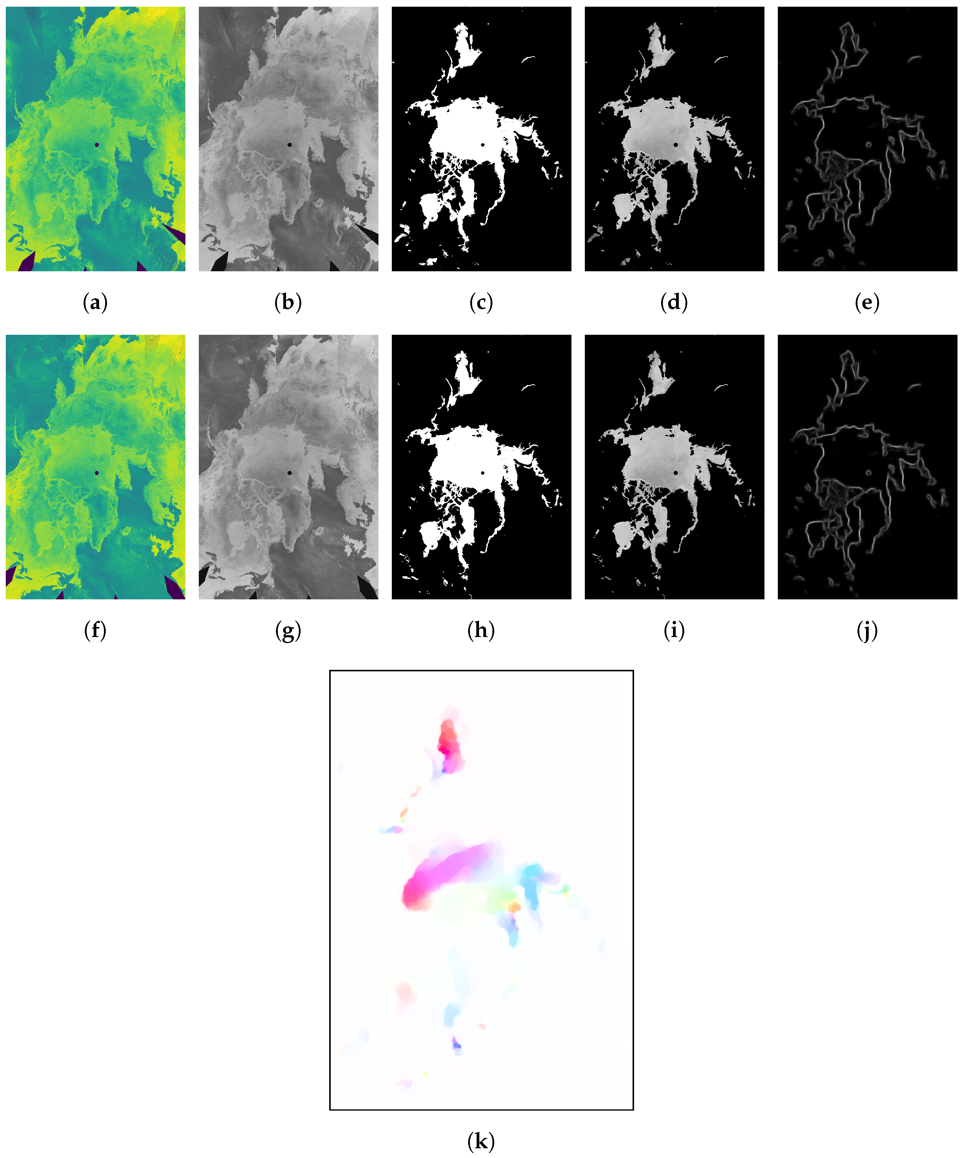
3.1. Optical Flow

Optical flow, a pivotal technique in image analysis, is employed to determine the motion of pixels between consecutive images. This method is extensively utilized in tasks such as image recognition, segmentation, and tracking [41,42]. A fundamental assumption of optical flow is the consistency in pixel motion, with only slight variations between successive images [43]. This technique negates the need for background scene modeling, focusing instead on pixel positional changes across the image series. By examining the correlation between pixels in successive images, the optical flow field is computed. This granular, pixel-wise approach is especially effective for capturing intricate sea ice deformations.

Taking into consideration that our dataset comprises AMSR-E images with dimensions of 608 pixels in width and 896 pixels in height, our primary objective is to achieve precise optical flow estimations. Sea ice motion is inherently intricate, influenced by numerous interrelated factors. Our future research direction is geared towards achieving real-time or near-real-time predictions of sea ice motion. Consequently, it is imperative to employ the EpicFlow method for computing optical flow between consecutive AMSR-E images. The EpicFlow method, proposed by Revaud et al. [44], calculates optical flow and is distinguished by the following characteristics:

• Efficiency : tailored for large-scale imagery, ensuring computational efficiency;
• Precision: offers high-accuracy optical flow estimations, capturing detailed pixel movements, ideal for tasks demanding precision such as object tracking and motion analysis;
• Versatility: applicable across various domains, from computer vision to autonomous driving, enhancing algorithmic performance and visual outcomes;
• Adaptability: excellently handles intricate motion scenarios and dynamic backdrops, managing swift and non-rigid motions and multiple object movements within scenes;
• Real-time capability: due to its efficiency and precision, it is apt for real-time applications, facilitating instantaneous visual feedback.

The computational process of EpicFlow commences with two input images. Matches are determined using DeepMatching [45], and edges from the initial image are extracted using SED [46]. These data points are subsequently employed for high-density match interpolation, producing a detailed dense correspondence field that initializes a single-level energy minimization framework. Figure 2 provides an overview of the key steps in the EpicFlow procedure.

In our study, we first convert all 280 original AMSR-E images into 8-bit grayscale format to simplify calculations and reduce the impact of noise on the results. We use AMSR-E data products that include daily sea ice concentration data, which is generated using the NASA Team 2 (NT2) algorithm [47]. Grid cells with a value of 0 represent open water, cells with a value of 110 indicate missing data, and cells with a value of 120 correspond to land. Grid cells with values between 1 and 100 represent percentages of sea ice concentration. Consequently, we employ this sea ice concentration data to create daily sea ice masks, effectively removing areas from each grayscale image that are not related to sea ice. Subsequently, we apply the EpicFlow algorithm to calculate optical flow on these masked images. Figure 3 exemplifies the application of EpicFlow on consecutive AMSR-E brightness temperature images.

3.2. Network Architecture

We introduce the SA-ConvLSTM architecture, a fusion of the ConvLSTM and a Self-Attention Memory Module (SAM), to enhance predictive capabilities for large-scale and long-term spatiotemporal sequence forecasting [25]. This architecture captures both global and local spatial dependencies concurrently.

3.2.1. SAM Module

The SAM module employs a novel memory unit, denoted as $\mathrm{M}$, to encapsulate spatial information infused with temporal dependencies. Inputs to the SAM module include the ConvLSTM-derived hidden layer state, ${\mathrm{H}}_{\mathrm{t}}$, from the current time step and the memory, ${\mathrm{M}}_{\mathrm{t}-1}$, from the preceding time step.

Initially, the SA mechanism processes ${\mathrm{H}}_{\mathrm{t}}$ to produce the feature, ${\mathrm{Z}}_{\mathrm{h}}$. This mechanism accentuates the significance of specific components within ${\mathrm{H}}_{\mathrm{t}}$. Simultaneously, ${\mathrm{H}}_{\mathrm{t}}$ acts as the Query, and ${\mathrm{M}}_{\mathrm{t}-1}$ is processed through the attention mechanism to produce the feature, ${\mathrm{Z}}_{\mathrm{m}}$. This emphasizes elements in ${\mathrm{H}}_{\mathrm{t}}$ with pronounced dependencies on ${\mathrm{M}}_{\mathrm{t}-1}$. By concatenating ${\mathrm{Z}}_{\mathrm{h}}$ and ${\mathrm{Z}}_{\mathrm{m}}$, we derive the aggregated feature, $\mathrm{Z}$, which embodies information from the current time step and global spatiotemporal memory.

Subsequently, the aggregated feature, $\mathrm{Z}$, interfaces with the gating structure found in LSTM to update both the hidden layer state and memory unit. This results in the updated hidden layer state, ${\widehat{\mathrm{H}}}_{\mathrm{t}}$, and the current time step memory, ${\mathrm{M}}_{\mathrm{t}}$. The formula for the SAM module is as follows:

$$\begin{array}{cc}\hfill & {\mathrm{i}}_{\mathrm{t}}^{\prime }=\sigma \left({\mathrm{W}}_{\mathrm{m};\mathrm{zi}}\ast \mathrm{Z}+{\mathrm{W}}_{\mathrm{m};\mathrm{hi}}\ast {\mathrm{H}}_{\mathrm{t}}+{\mathrm{b}}_{\mathrm{m};\mathrm{i}}\right)\hfill \\ \hfill & {\mathrm{g}}_{\mathrm{t}}^{\prime }=tanh\left({\mathrm{W}}_{\mathrm{m};\mathrm{zg}}\ast \mathrm{Z}+{\mathrm{W}}_{\mathrm{m};\mathrm{hg}}\ast {\mathrm{H}}_{\mathrm{t}}+{\mathrm{b}}_{\mathrm{m};\mathrm{g}}\right)\hfill \\ \hfill & {\mathrm{M}}_{\mathrm{t}}=\left(1-{\mathrm{i}}_{\mathrm{t}}^{\prime }\right)\circ {\mathrm{M}}_{\mathrm{t}-1}+{\mathrm{i}}_{\mathrm{t}}^{\prime }\circ {\mathrm{g}}_{\mathrm{t}}^{\prime }\hfill \\ \hfill & {\mathrm{o}}_{\mathrm{t}}^{\prime }=\sigma \left({\mathrm{W}}_{\mathrm{m};\mathrm{zo}}\ast \mathrm{Z}+{\mathrm{W}}_{\mathrm{m};\mathrm{ho}}\ast {\mathrm{H}}_{\mathrm{t}}+{\mathrm{b}}_{\mathrm{m};\mathrm{o}}\right)\hfill \\ \hfill & {\widehat{\mathrm{H}}}_{\mathrm{t}}={\mathrm{o}}_{\mathrm{t}}^{\prime }\circ {\mathrm{M}}_{\mathrm{t}}\hfill \end{array}$$

(1)

In the above equations:

• ${\mathrm{i}}_{\mathrm{t}}^{\prime }$ represents the input gate. It is a value processed through the sigmoid function and controls how much of the new information ${\mathrm{g}}_{\mathrm{t}}^{\prime }$ should be added to the memory ${\mathrm{M}}_{\mathrm{t}}$. This gate mechanism determines how much of the previous memory should be retained in the current time step $\mathrm{t}$.
• ${\mathrm{g}}_{\mathrm{t}}^{\prime }$ represents new memory candidate values, processed through the hyperbolic tangent function. It indicates the new information to be added to the memory ${\mathrm{M}}_{\mathrm{t}}$.
• ${\mathrm{M}}_{\mathrm{t}}$ is the memory at the current time step $\mathrm{t}$. Memory serves as the model’s internal state and is responsible for storing information about the input sequence. Its update is controlled by the input gate ${\mathrm{i}}_{\mathrm{t}}^{\prime }$ and the new information ${\mathrm{g}}_{\mathrm{t}}^{\prime }$, as well as the forgetting of the previous time step’s memory ${\mathrm{M}}_{\mathrm{t}-1}$.
• ${\mathrm{o}}_{\mathrm{t}}^{\prime }$ is the output gate. It is a value processed through the sigmoid function and controls how the information in the memory ${\mathrm{M}}_{\mathrm{t}}$ affects the output. This gate mechanism determines how much memory information should influence the output value ${\widehat{\mathrm{H}}}_{\mathrm{t}}$.
• ${\widehat{\mathrm{H}}}_{\mathrm{t}}$ is the output at time step $\mathrm{t}$ and is obtained by multiplying the memory ${\mathrm{M}}_{\mathrm{t}}$ with the output gate ${\mathrm{o}}_{\mathrm{t}}^{\prime }$. This determines the impact of memory information on the model’s output.
• The weight matrices ${\mathrm{W}}_{\mathrm{m};\mathrm{zi}}$, ${\mathrm{W}}_{\mathrm{m};\mathrm{hi}}$, ${\mathrm{W}}_{\mathrm{m};\mathrm{zg}}$, ${\mathrm{W}}_{\mathrm{m};\mathrm{hg}}$, ${\mathrm{W}}_{\mathrm{m};\mathrm{zo}}$ and ${\mathrm{W}}_{\mathrm{m};\mathrm{ho}}$ along with bias terms ${\mathrm{b}}_{\mathrm{m};\mathrm{i}}$, ${\mathrm{b}}_{\mathrm{m};\mathrm{g}}$ and ${\mathrm{b}}_{\mathrm{m};\mathrm{o}}$ are parameters used to control the gating and memory updates.

The SAM Module provides an additional value in the SA-ConvLSTM network by enhancing the network’s ability to capture long-range dependencies and contextual information within the input data. It achieves this by allowing the network to focus on specific regions or features of the input sequence that are most relevant for making predictions at each time step. This attention mechanism helps the network adaptively weigh the importance of different spatial and temporal elements, thus improving its ability to model complex patterns and relationships within the data. It can capture dependencies that may span a considerable time horizon, which is particularly valuable in tasks where distant interactions or dependencies are crucial for accurate predictions, such as in time series forecasting, natural language processing, or image analysis.

3.2.2. Base Model

The base network model seamlessly integrates Self-Attention and ConvLSTM through direct cascading. The model is formulated as follows:

$$\begin{array}{cc}\hfill {\widehat{\mathrm{X}}}_{\mathrm{t}}& =\mathrm{SA}\left({\mathrm{X}}_{\mathrm{t}}\right),{\widehat{\mathrm{H}}}_{\mathrm{t}-1}=\mathrm{SA}\left({\mathrm{H}}_{\mathrm{t}-1}\right)\hfill \\ \hfill {\mathrm{i}}_{\mathrm{t}}& =\sigma \left({\mathrm{W}}_{\mathrm{xi}}\ast {\widehat{\mathrm{X}}}_{\mathrm{t}}+{\mathrm{W}}_{\mathrm{hi}}\ast {\widehat{\mathrm{H}}}_{\mathrm{t}-1}+{\mathrm{b}}_{\mathrm{i}}\right)\hfill \\ \hfill {\mathrm{f}}_{\mathrm{t}}& =\sigma \left({\mathrm{W}}_{\mathrm{xf}}\ast {\widehat{\mathrm{X}}}_{\mathrm{t}}+{\mathrm{W}}_{\mathrm{hf}}\ast {\widehat{\mathrm{H}}}_{\mathrm{t}-1}+{\mathrm{b}}_{\mathrm{f}}\right)\hfill \\ \hfill {\mathrm{g}}_{\mathrm{t}}& =tanh\left({\mathrm{W}}_{\mathrm{xc}}\ast {\widehat{\mathrm{X}}}_{\mathrm{t}}+{\mathrm{W}}_{\mathrm{hc}}\ast {\widehat{\mathrm{H}}}_{\mathrm{t}-1}+{\mathrm{b}}_{\mathrm{c}}\right)\hfill \\ \hfill {\mathrm{C}}_{\mathrm{t}}& ={\mathrm{f}}_{\mathrm{t}}\circ {\mathrm{C}}_{\mathrm{t}-1}+{\mathrm{i}}_{\mathrm{t}}\circ {\mathrm{g}}_{\mathrm{t}}\hfill \\ \hfill {\mathrm{o}}_{\mathrm{t}}& =\sigma \left({\mathrm{W}}_{\mathrm{xo}}\ast {\widehat{\mathrm{X}}}_{\mathrm{t}}+{\mathrm{W}}_{\mathrm{ho}}\ast {\widehat{\mathrm{H}}}_{\mathrm{t}-1}+{\mathrm{b}}_{\mathrm{o}}\right)\hfill \\ \hfill {\mathrm{H}}_{\mathrm{t}}& ={\mathrm{o}}_{\mathrm{t}}\circ tanh\left({\mathrm{C}}_{\mathrm{t}}\right),\hfill \end{array}$$

(2)

In the above equations:

• $\mathrm{SA}$ represents the self-attention module.
• ${\widehat{\mathrm{X}}}_{\mathrm{t}}$ represents the result of applying a Self-Attention module to the input ${\mathrm{X}}_{\mathrm{t}}$ at time step $\mathrm{t}$. Self-Attention helps the model capture relationships between different elements in the input sequence.
• ${\widehat{\mathrm{H}}}_{\mathrm{t}-1}$ is the result of applying a Self-Attention module to the previous time step’s hidden state ${\mathrm{H}}_{\mathrm{t}-1}$. It aids the model in capturing internal relationships within the hidden state.
• ${\mathrm{i}}_{\mathrm{t}}$ represents the input gate. It is a value processed through the sigmoid function ($\sigma$) and controls how much of the new information ${\mathrm{g}}_{\mathrm{t}}$ should be added to the cell state ${\mathrm{C}}_{\mathrm{t}}$.
• ${\mathrm{f}}_{\mathrm{t}}$ is the forget gate. The forget gate, also processed through the sigmoid function, determines how much information from the previous time step’s cell state ${\mathrm{C}}_{\mathrm{t}-1}$ should be retained in the current time step.
• ${\mathrm{g}}_{\mathrm{t}}$ represents new information, which is processed through the hyperbolic tangent (tanh) function. It is used to calculate the value to be added to the cell state ${\mathrm{C}}_{\mathrm{t}}$ and serves as a candidate cell state.
• ${\mathrm{C}}_{\mathrm{t}}$ is the cell state. It is the internal memory of the LSTM unit and stores information about the input data. The forget gate ${\mathrm{f}}_{\mathrm{t}}$ controls what information is retained and forgotten from the previous time step’s cell state, while ${\mathrm{i}}_{\mathrm{t}}$ and ${\mathrm{g}}_{\mathrm{t}}$ control the addition of new information.
• ${\mathrm{o}}_{\mathrm{t}}$ is the output gate. It is a value processed through the sigmoid function and determines the extent to which information from the cell state ${\mathrm{C}}_{\mathrm{t}}$ is passed to the hidden state ${\mathrm{H}}_{\mathrm{t}}$.
• ${\mathrm{H}}_{\mathrm{t}}$ is the hidden state at time step $\mathrm{t}$. It is the primary output of the LSTM unit. It is obtained by multiplying the cell state ${\mathrm{C}}_{\mathrm{t}}$ by the output gate ${\mathrm{o}}_{\mathrm{t}}$ and processing the result through the hyperbolic tangent function.
• ${\mathrm{W}}_{\mathrm{xi}}$, ${\mathrm{W}}_{\mathrm{xf}}$, ${\mathrm{W}}_{\mathrm{xc}}$, ${\mathrm{W}}_{\mathrm{xo}}$, ${\mathrm{W}}_{\mathrm{hi}}$, ${\mathrm{W}}_{\mathrm{hf}}$, ${\mathrm{W}}_{\mathrm{hc}}$, ${\mathrm{W}}_{\mathrm{ho}}$ are weight matrices that are used to linearly combine the transformed input sequence and the previous hidden state to compute the input gate, forget gate, candidate cell state value, and output gate. These weight matrices are learned as model parameters during training. ${\mathrm{b}}_{\mathrm{i}}$, ${\mathrm{b}}_{\mathrm{f}}$, ${\mathrm{b}}_{\mathrm{c}}$, ${\mathrm{b}}_{\mathrm{o}}$ are bias terms that help adjust the behavior of the gates and the computation of the candidate cell state, similar to a standard LSTM. These bias terms are also learned as model parameters during training.

The above formula represents the data processing process of the input data in the SA-ConvLSTM base model. More specifically, when we are given the input of the sea ice motion vector field, the basic model’s data processing can be decomposed into two main components: the Self-Attention application and ConvLSTM operations.

In the Self-Attention application, the sea ice motion vector data at time step $\mathrm{t}$, represented by ${\mathrm{X}}_{\mathrm{t}}$, is first processed by the Self-Attention mechanism to produce ${\widehat{\mathrm{X}}}_{\mathrm{t}}$. This step allows the model to assign different weights to different parts of the input based on their spatial and temporal relevance, emphasizing regions with significant ice movement or patterns. Similarly, the hidden state from the previous time step, ${\mathrm{H}}_{\mathrm{t}-1}$, is transformed by the Self-Attention mechanism to produce ${\widehat{\mathrm{H}}}_{\mathrm{t}-1}$. This ensures that the model can recognize and leverage patterns and dependencies from its own previous states.

In the ConvLSTM operations, using the Self-Attention processed sea ice motion vector data ${\widehat{\mathrm{X}}}_{\mathrm{t}}$ and hidden state ${\widehat{\mathrm{H}}}_{\mathrm{t}-1}$, the model computes the input gate ${\mathrm{i}}_{\mathrm{t}}$, forget gate ${\mathrm{f}}_{\mathrm{t}}$, new information ${\mathrm{g}}_{\mathrm{t}}$, and the output gate ${\mathrm{o}}_{\mathrm{t}}$. These gates regulate the flow of information through the cell, determining which patterns to retain or discard. The cell state ${\mathrm{C}}_{\mathrm{t}}$ is updated using the gates and the new information. This state acts as the LSTM’s memory, preserving essential patterns from the sea ice motion vector data and discarding irrelevant details. The hidden state ${\mathrm{H}}_{\mathrm{t}}$ for the current time step is then derived using the cell state and the output gate. This hidden state can be used for subsequent processing or predictions, representing the model’s understanding of the sea ice motion at that time step.

The Self-Attention mechanism allows the model to focus on important parts of the sea ice motion vector data based on their spatial and temporal relevance. This ensures the model adeptly highlights crucial ice movement patterns and downplays less pertinent ones. The SA-ConvLSTM can understand global spatial relationships across RNN layers and states, essential for understanding sea ice dynamics and making predictions. While Self-Attention may increase computational needs, the model’s design, especially with segmented optical flow images, ensures these demands remain manageable. This is vital for the efficient processing of high-definition sea ice motion vector data.

3.2.3. SA-ConvLSTM

The SA-ConvLSTM architecture represents a groundbreaking fusion of Self-Attention mechanisms with ConvLSTM networks. By integrating the SAM into the ConvLSTM framework, as illustrated in Figure 4, the architecture elevates its capability to process sequential data with spatial nuances. Central to this is the SAM’s ability to identify and prioritize distinct spatial features, enabling the model to focus on key patterns, thereby enhancing its predictive accuracy.

Fundamentally, the SA-ConvLSTM model combines Self-Attention and ConvLSTM, making it ideal for the sea ice motion dataset. This blend captures spatial and temporal data aspects, deepening insights into sea ice dynamics and improving predictions. The model balances Self-Attention with LSTM to retain key patterns and discard irrelevant details, enhancing performance in understanding complex sea ice dynamics. By integrating Self-Attention and ConvLSTM, the model benefits from both: ConvLSTM captures local patterns, while Self-Attention provides a wider context, improving the model’s understanding of sea ice movements.

The inclusion of SAM in the ConvLSTM is not just a mere layer addition. It reshapes the model’s data processing. SA-ConvLSTM emphasizes adaptability. Its structure permits easy removal of the SAM, allowing a smooth return to classic ConvLSTM. This adaptability benefits developers and researchers, letting them tailor the model’s depth to specific needs. Whether needing SAM’s advanced insights for complex data or the efficiency of standard ConvLSTM for basic tasks, SA-ConvLSTM stands out as a flexible tool.

3.3. Network Parameters

Our prediction model is trained using data from AMSR-E. It leverages daily optical flow vectors generated by the EpicFlow method, resulting in a multitude of sequences, each comprising 20 consecutive daily arrays. In these sequences, the initial ten arrays serve as inputs, while the model predicts the subsequent ten arrays as outputs.

To create the validation set, we randomly select time-overlapping sequences during network training. To ensure that there is no overlap with the validation set, we take care to exclude any sequences with common dates. Additionally, we create a separate test set by randomly selecting another batch of time-overlapping sequences. The remaining sequences, with no shared dates with the validation and test sets, constitute the training set. Each sequence is divided into 32 × 32 subsequences, corresponding to different times but representing the same spatial region across the width and height of the image.

To enhance both training efficiency and accuracy, we exclude sequences devoid of sea ice pixels from our training set, validation set, and test set. It is worth noting that a prior study [21] retained non-sea ice pixels, such as land, in the training and validation sets. However, this approach could potentially hinder training efficiency and lead to confusion between land and sea ice in prediction results. Consequently, our training and validation sets exclusively contain sea ice pixels, encompassing both moving and non-moving sea ice.

Following the aforementioned process, we generated an ice velocity dataset with dimensions (279, 896, 608, 2). The number 279 represents the total number of optical flow vector fields obtained after calculating the flow between adjacent frames from the original set of 280 images. The dimensions 896 and 608 correspond to the height and width of each vector field, respectively, and the ‘2’ signifies that each vector contains velocity information in both the x and y directions. Given the vast size of this dataset, it cannot be directly utilized as input for training the SA-ConvLSTM network. Therefore, data segmentation is necessary. Since 32 is the greatest common divisor of 896 and 608, we have chosen 32 as the minimum unit for slicing. Each vector field can be sliced into 532 smaller 32 × 32 blocks, each with dimensions (32, 32, 2). Patches devoid of pixels falling within the sea ice mask area are excluded from the dataset. Subsequently, the dataset is randomly shuffled, and 80% of it is designated as the training set, while 10% is allocated to both the testing and validation sets, ensuring complete separation between the three sets. After this rigorous preparation, we ultimately obtain the entire dataset, which comprises 33,404 sequences, each consisting of 20 consecutive daily images. Out of these, 26,724 sequences are utilized for training, while 3340 sequences are assigned to both the testing and validation sets.

To mitigate the adverse effects stemming from singular sample data and accelerate convergence, we employ maximum–minimum normalization to map the data into the [0, 1] range before initiating model training. Within the network architecture, linear output units are employed in the SA-ConvLSTM network, as the required output consists of optical flow real values. The weight matrices are initialized by sampling from a uniform distribution, and biases are set to zero. To strike a balance between model complexity and computational efficiency, our SA-ConvLSTM model is structured with a three-layer architecture. Adding more layers can enhance the model’s representational capacity but may also lead to overfitting and increased computational costs. Each layer consists of 128 hidden states to provide sufficient capacity for learning and representing complex patterns in the data. The convolutional kernel size is set to 5 × 5 to ensure the capture of local spatial patterns and to have a sufficient receptive field to consider the surrounding context. The number of network layers and the convolutional kernel size are consistent with the study [21]. Model training is conducted using the ADAM optimizer, with an initial learning rate of 0.001, in alignment with a similar study [25]. After multiple experiments, we find that setting the mini-batch size to 8 yields the best performance on the validation set. The model converges quickly, thus providing a good balance between computational efficiency and model performance. Additionally, to prevent overfitting, we implement an early stopping mechanism by monitoring the ‘val_loss’ parameter. Training halts when improvements become marginal, with a minimum delta (’min_delta’) of 0.0001 and a patience setting of 5. The mode is set to ‘min’, and we retain the best weights using the ‘restore_best_weights’ parameter. In our training process, we employ the L2 loss function.

4. Results

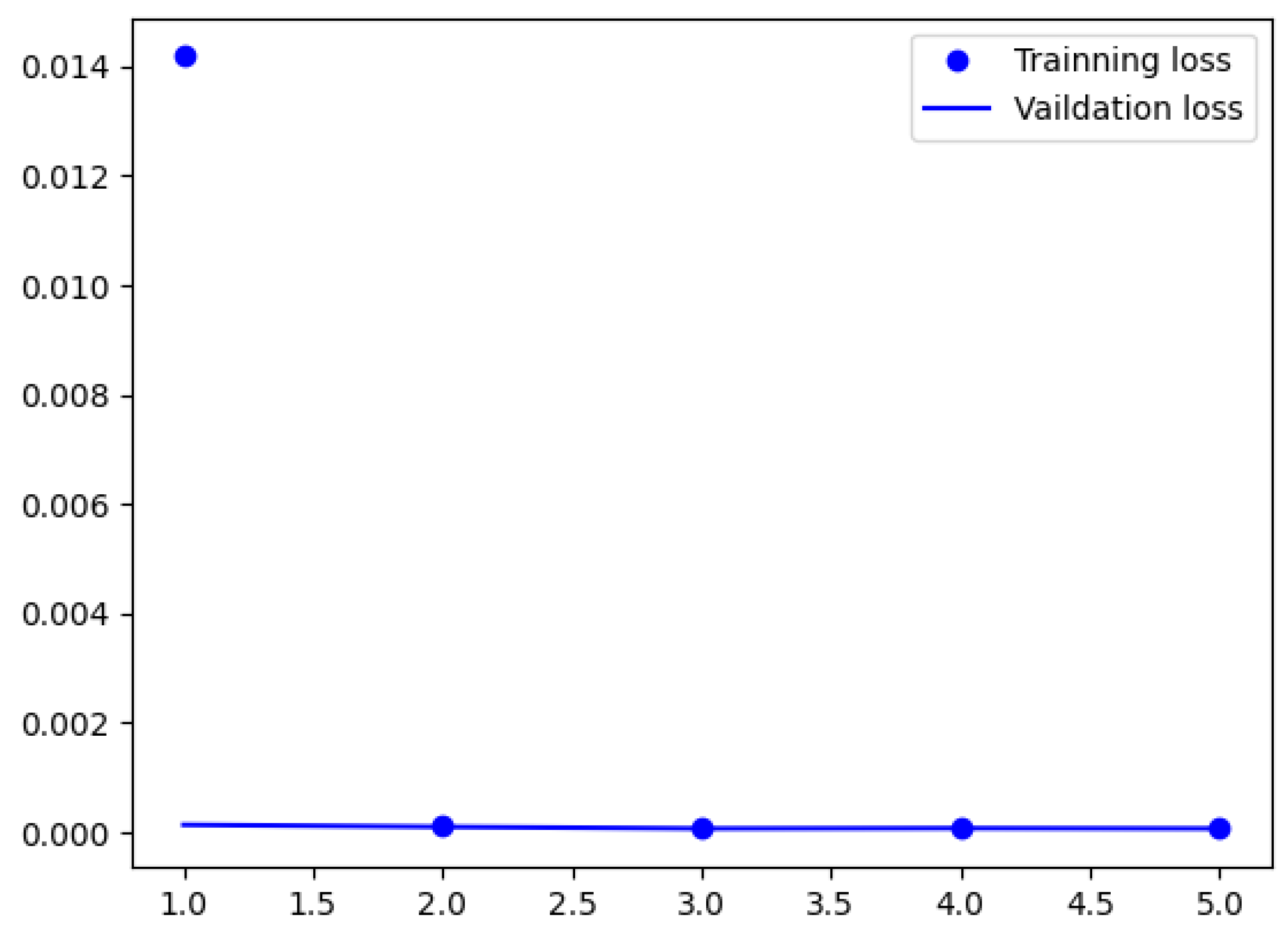
4.1. Training Results

Figure 5 and Figure 6 display the mean squared error (MSE) and mean absolute error (MAE) across epochs during the training process. Our model’s training process was stopped early, after only 5 epochs. Recent studies have demonstrated that adding the Self-Attention mechanism to the model can significantly improve its convergence speed [48,49,50,51,52]. During this short training period, the training loss rapidly decreased to 9.6016 ×${10}^{-5}$ and then remained stable with minor fluctuations. The validation loss followed a similar pattern, maintaining a nearly constant value around 9.6016 ×${10}^{-5}$. The changes in training MAE appeared to mirror the training loss. Notably, during the third and fourth epochs, the validation MAE experienced slight fluctuations but quickly stabilized. Our model has a total of 8,306,946 parameters, with 8,306,178 of them being trainable and 768 being non-trainable. On the test set, our model achieved a loss of 8.6046 ×${10}^{-5}$ and a MAE of 0.005. These results indicate that the model fits the training data well, and its performance on both the validation and test sets suggests that it has not overfitted.

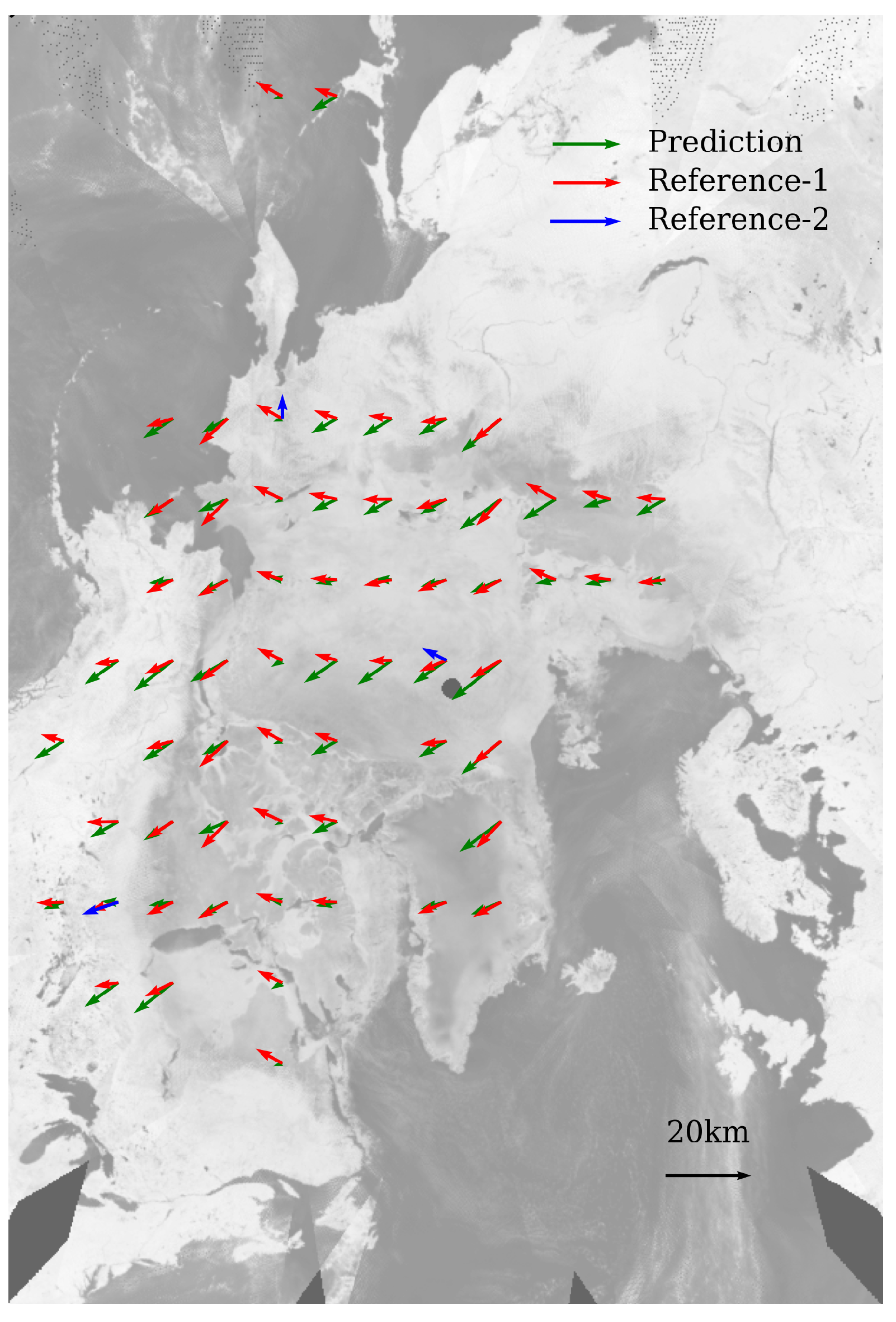
4.2. Comparison with Reference Optical Flow

In our experiments, we employ the first 10 optical flow patches from each test set sequence as inputs to predict the subsequent 10 patches. Initially, we compare the predicted optical flow with the reference optical flow patches for both the x and y motion axes at each pixel location. Pixels outside the sea ice zone are excluded from the comparison. Figure 7 illustrates the error statistics for each future prediction step. For instance, if the input comprises patches from days 1–10, step 1 represents the prediction patch for day 11, step 2 for day 12, and so on. After eliminating non-sea ice pixels, approximately 700,000 pixels are retained for each prediction step.

Table 2. Comparison of the predicted motion and the reference optical flow in the entire Arctic, for each prediction step in the future (fut). RMSE and MAE are in km.

	x Axis			y Axis
Fut	RMSE	MAE	RMSE-MAE	RMSE	MAE	RMSE-MAE
1	1.17	1.15	0.02	0.91	0.87	0.04
2	1.57	1.55	0.02	1.34	1.31	0.03
3	1.85	1.82	0.03	1.67	1.64	0.02
4	2.03	1.99	0.04	1.91	1.88	0.03
5	2.09	2.05	0.04	2.00	1.96	0.04
6	2.12	2.08	0.04	2.03	2.00	0.03
7	2.14	2.10	0.04	2.06	2.02	0.04
8	2.15	2.11	0.04	2.07	2.03	0.04
9	2.16	2.12	0.04	2.08	2.04	0.04
10	2.17	2.13	0.04	2.09	2.05	0.04
Avg.	1.94	1.91	0.035	1.81	1.78	0.035

provides a clear representation of the accuracy of motion prediction compared to the reference optical flow. Unsurprisingly, the initial prediction step stands out as the most accurate, with the minimum error observed in both motion axes. As we project our predictions further into the future, the trend becomes evident: during the first three days, there is a notable and rapid increase in prediction error. This is followed by a more gradual and steady rise over the subsequent seven days.

It is important to note that, despite this gradual decline in performance, our model consistently maintains a high level of accuracy. Even after 10 prediction steps, which is a substantial time horizon, the error values remain impressively low and exhibit remarkable stability. This robust performance over an extended forecast horizon highlights the model’s reliability and suitability for applications requiring accurate optical flow predictions.

4.3. Comparison with Drift Data Inherent in the AMSR-E Product

To comprehensively evaluate the accuracy of our proposed method, we conducted a comparative analysis by assessing the predicted motion against the drift data inherent in the source AMSR-E data product. This product includes daily sea ice drift data derived from the maximum cross correlation (MCC) feature tracking algorithm developed by the University of Colorado (CU). The basic method of this algorithm is quite simple. Two spatially coincident images were obtained, which were separated by a period of time. Select the target area in the first (old) image that can be defined by pixels or pixel groups. Then, select the search area around the target area in the second (newer) image. Compare the correlation with the target region in the first image with all regions (the size of the target region) in the search area of the second image. The area with the highest correlation is determined as the location of the target movement. A filtering algorithm is then used to remove at least some problematic matches.

To be more specific, Gridded Level 3 daily composite ${\mathrm{T}}_{\mathrm{b}}\mathrm{s}$ at 12.5 km on the polar stereographic grid are used as input for the MCC algorithm. Ice motions are calculated from two composite images using the sliding window to find the correlation peak, which determines the distance a feature has moved. The drift is then computed by dividing the distance by the time separation (24 h). A sea ice mask is applied to only retrieve ice motion where concentration is above the standard sea ice extent threshold of 15% concentration. False correlations can occur due to clouds or variability of ice surface features. To eliminate this, first a minimum correlation threshold of 0.7 is applied to eliminate weak matches. Next a post-processing filter program is run to remove at least some questionable and erroneous motions. This uses the fact that motion is highly spatially correlated and requires that each vector be reasonably consistent in speed and direction with at least two neighboring motion estimates.

Table 3. Accuracy evaluation of the predicted motion versus drift data inherent in original AMSR-E data product in the entire Arctic, for each prediction step in the future (fut). RMSE and MAE are in km.

	x Axis			y Axis
Fut	RMSE	MAE	RMSE-MAE	RMSE	MAE	RMSE-MAE
1	1.80	1.64	0.16	1.30	1.06	0.24
2	2.56	2.44	0.12	2.11	1.94	0.17
3	3.10	2.97	0.13	2.74	2.58	0.16
4	3.46	3.32	0.14	3.22	3.06	0.16
5	3.58	3.44	0.14	3.38	3.22	0.16
6	3.65	3.49	0.16	3.45	3.30	0.15
7	3.68	3.53	0.15	3.50	3.34	0.16
8	3.71	3.56	0.15	3.53	3.37	0.16
9	3.73	3.57	0.16	3.55	3.39	0.16
10	3.75	3.59	0.16	3.57	3.41	0.16
Avg.	3.30	3.15	0.147	3.03	2.86	0.168

shows the errors between our prediction vectors and the motion vectors from AMSR-E data product in the future 10 days. As anticipated, the data reveals a distinct trend in prediction accuracy. Initially, on the first day of prediction, our model achieves the lowest error in motion prediction, indicating a high degree of accuracy for short-term forecasts. However, as the forecast horizon extends into the future, we observe a gradual increase in prediction error. This trend is a common characteristic of predictive models, as the inherent uncertainties in longer-term predictions become more pronounced.

It is important to note a significant difference when comparing the data in Table 3 with that in Table 2: the average MAE and RMSE values are consistently higher by approximately 1.0–1.3 km in Table 3. The difference between the two tables can be attributed to the inherent characteristics of the MCC feature tracking algorithm and the optical flow method. The MCC algorithm tends to produce a sparse drift velocity field. This sparsity presents a challenge when attempting to obtain comprehensive, large-scale continuous drift estimates. In contrast, the optical flow method generates a denser optical flow field. This higher density of information contributes to the relatively more accurate predictions observed in Table 2. This emphasizes the importance of choosing the appropriate algorithm for specific applications in sea ice prediction.

A remarkable distinction arises when examining the errors along the x axis (latitude) and y axis (longitude) in both Table 2 and Table 3. Specifically, the errors along the x-axis are consistently higher than those along the y-axis. This observation implies that predicting sea ice movement in the latitude direction (x-axis) is inherently more challenging compared to predictions in the longitude direction (y-axis). This difference could be attributed to various factors, including the complex interplay of environmental variables, ocean currents, and atmospheric conditions that influence sea ice drift differently in these two directions. This underscores the imperative for additional research and refinement to more comprehensively grasp the intricacies of sea ice movement in both geographical axes.

4.4. Comparison with Previous Methods

Our SA-ConvLSTM model is also compared with RNN [17] and ConvLSTM [21] on the AMSR-E data, as detailed in

Table 4. Comparison with previous deep learning methods. RMSE and MAE are in km.

	x Axis		y Axis
Method	RMSE	MAE	RMSE	MAE
baseline	4.94	3.61	4.43	3.10
[17]	4.53	3.36	3.71	2.68
[21]	4.21	3.09	3.71	2.58
Ours	1.94	1.91	1.81	1.78

. To provide a baseline for reference, we also consider a simple approach of replicating the last observed input optical flow. The aggregated results are summarized in Table 4, where the average errors for predicting Arctic sea ice motion over 10 future time steps are presented.

Notably, our SA-ConvLSTM network outperforms both the fully connected conditional LSTM network [17] and the ConvLSTM network [21] when relying solely on the AMSR-E data source. Compared to ConvLSTM, our method shows a reduction of 0.80 to 1.18 km in average MAE over a 10-day period. This achievement underscores the effectiveness of incorporating a Self-Attention Memory (SAM) module into the ConvLSTM architecture. The SAM module enhances the model’s capacity to capture spatiotemporal information, particularly at small and medium scales. These findings carry significant promise for future research endeavors focused on developing more precise unsupervised learning methods for Arctic sea ice prediction. An especially promising research direction involves the expansion of similar models to handle larger-scale applications, which could potentially lead to even more accurate predictions.

4.5. Visualization Example

Figure 8 presents a comparative example between the step 1 prediction vector and the reference optical flow. To facilitate visualization, a close-up of the original image range is displayed, with vectors drawn at intervals of 56 pixels vertically and 38 pixels horizontally. These vectors are magnified 20 times to ensure clear visibility. While it is worth noting that in some instances, the predicted motion vectors slightly underestimate the true amplitude of the reference optical flow vector orientation, overall, they exhibit a strong correlation. In conclusion, the quantitative results presented above, in combination with this visual assessment, underscore the effectiveness of the proposed method, which combines SA-ConvLSTM with optical flow, in delivering satisfactory predictions for future sea ice movement. This approach indeed represents a promising avenue for further research in the field.

5. Conclusions

In this paper, we have presented a novel approach to predict sea ice motion using the SA-ConvLSTM network and optical flow input, leveraging only satellite AMSR-E single source data. Our methodology takes advantage of past relevant features to enhance the prediction of the current time step. We have achieved this by constructing a Self-Attention Memory module capable of capturing long-range dependencies in both spatial and temporal dimensions. We have extensively compared our model against both reference optical flow data and motion vectors extracted from the AMSR-E data product. Our results indicate that our model consistently provides satisfactory predictions for Arctic sea ice motion over the next 10 days.

Notably, our proposed approach outperforms previous ConvLSTM-based multistep prediction methods. Despite being trained exclusively on sparse-resolution reference flow data, our model demonstrates remarkable accuracy and stability. As a consequence, our method presents a promising alternative or complementary approach for complex numerical models that traditionally rely on multi-source data.

Moreover, our method is particularly well-suited for predicting motion vector fields at lower resolutions or small to medium-sized scales. For the prediction of high-resolution vector fields, additional preprocessing steps are required, such as cutting the fields into smaller segments and concatenating the output prediction results. Looking ahead, our future work will focus on extending our prediction methods to address the challenges posed by large-scale sea ice motion vector fields. We believe that further research in this direction will continue to advance our understanding and prediction capabilities in the field of sea ice dynamics. The data used in our study can be downloaded from [53] https://doi.org/10.6084/m9.figshare.24354901.v3.

References

- Meredith, M.; Sommerkorn, M.; Cassotta, S.; Derksen, C.; Ekaykin, A.; Hollowed, A.; Kofinas, G.; Mackintosh, A.; Melbourne-Thomas, J.; Muelbert, M.; et al. Polar regions. In IPCC Special Report on the Ocean and Cryosphere in a Changing Climate; IPCC: Geneva, Switzerland, 2019; Chapter 3. [Google Scholar]
- Pithan, F.; Mauritsen, T. Arctic amplification dominated by temperature feedbacks in contemporary climate models. Nat. Geosci. 2014, 7, 181–184. [Google Scholar] [CrossRef]
- Zhang, Y.F.; Bushuk, M.; Winton, M.; Hurlin, B.; Delworth, T.; Harrison, M.; Jia, L.; Lu, F.; Rosati, A.; Yang, X. Subseasonal-to-Seasonal Arctic Sea Ice Forecast Skill Improvement from Sea Ice Concentration Assimilation. J. Clim. 2022, 35, 4233–4252. [Google Scholar] [CrossRef]
- Smith, G.C.; Liu, Y.; Benkiran, M.; Chikhar, K.; Surcel Colan, D.; Gauthier, A.A.; Testut, C.E.; Dupont, F.; Lei, J.; Roy, F.; et al. The Regional Ice Ocean Prediction System v2: A pan-Canadian ocean analysis system using an online tidal harmonic analysis. Geosci. Model Dev. 2021, 14, 1445–1467. [Google Scholar] [CrossRef]
- Dirkson, A.; Merryfield, W.J.; Monahan, A. Impacts of sea ice thickness initialization on seasonal Arctic sea ice predictions. J. Clim. 2017, 30, 1001–1017. [Google Scholar] [CrossRef]
- Lavergne, T.; Down, E. A Climate Data Record of Year-Round Global Sea Ice Drift from the EUMETSAT OSI SAF. Earth Syst. Sci. Data Discuss. 2023, 1–38. [Google Scholar]
- Schweiger, A.J.; Zhang, J. Accuracy of short-term sea ice drift forecasts using a coupled ice-ocean model. J. Geophys. Res. Ocean. 2015, 120, 7827–7841. [Google Scholar] [CrossRef]
- Hebert, D.A.; Allard, R.A.; Metzger, E.J.; Posey, P.G.; Preller, R.H.; Wallcraft, A.J.; Phelps, M.W.; Smedstad, O.M. Short-term sea ice forecasting: An assessment of ice concentration and ice drift forecasts using the US Navy’s Arctic Cap Nowcast/Forecast System. J. Geophys. Res. Ocean. 2015, 120, 8327–8345. [Google Scholar] [CrossRef]
- Yang, C.Y.; Liu, J.; Xu, S. Seasonal Arctic sea ice prediction using a newly developed fully coupled regional model with the assimilation of satellite sea ice observations. J. Adv. Model. Earth Syst. 2020, 12, e2019MS001938. [Google Scholar] [CrossRef]
- De Silva, L.W.A.; Yamaguchi, H. Grid size dependency of short-term sea ice forecast and its evaluation during extreme Arctic cyclone in August 2016. Polar Sci. 2019, 21, 204–211. [Google Scholar] [CrossRef]
- Zampieri, L.; Goessling, H.F.; Jung, T. Bright prospects for Arctic sea ice prediction on subseasonal time scales. Geophys. Res. Lett. 2018, 45, 9731–9738. [Google Scholar] [CrossRef]
- Spreen, G.; Kwok, R.; Menemenlis, D. Trends in Arctic sea ice drift and role of wind forcing: 1992–2009. Geophys. Res. Lett. 2011, 38, L19501. [Google Scholar] [CrossRef]
- Mu, B.; Luo, X.; Yuan, S.; Liang, X. IceTFT v 1.0.0: Interpretable Long-Term Prediction of Arctic Sea Ice Extent with Deep Learning. Geosci. Model Dev. Discuss. 2023, 16, 4677–4697. [Google Scholar] [CrossRef]
- Liu, Q.; Zhang, R.; Wang, Y.; Yan, H.; Hong, M. Short-Term Daily Prediction of Sea Ice Concentration Based on Deep Learning of Gradient Loss Function. Front. Mar. Sci. 2021, 8, 736429. [Google Scholar] [CrossRef]
- Kim, Y.J.; Kim, H.C.; Han, D.; Lee, S.; Im, J. Prediction of monthly Arctic sea ice concentrations using satellite and reanalysis data based on convolutional neural networks. Cryosphere 2020, 14, 1083–1104. [Google Scholar] [CrossRef]
- Liu, Y.; Bogaardt, L.; Attema, J.; Hazeleger, W. Extended-range arctic sea ice forecast with convolutional long short-term memory networks. Mon. Weather Rev. 2021, 149, 1673–1693. [Google Scholar] [CrossRef]
- Petrou, Z.I.; Tian, Y. Prediction of sea ice motion with recurrent neural networks. In Proceedings of the 2017 IEEE International Geoscience and Remote Sensing Symposium (IGARSS), Fort Worth, TX, USA, 23–28 July 2017; IEEE: Piscataway, NJ, USA, 2017; pp. 5422–5425. [Google Scholar]
- Alqushaibi, A.; Abdulkadir, S.J.; Rais, H.M.; Al-Tashi, Q. A review of weight optimization techniques in recurrent neural networks. In Proceedings of the 2020 International Conference on Computational Intelligence (ICCI), Bandar Seri Iskandar, Malaysia, 8–9 October 2020; IEEE: Piscataway, NJ, USA, 2020; pp. 196–201. [Google Scholar]
- Zhai, J.; Bitz, C.M. A machine learning model of Arctic sea ice motions. arXiv 2021, arXiv:2108.10925. [Google Scholar]
- Farooque, G.; Xiao, L.; Yang, J.; Sargano, A.B. Hyperspectral image classification via a novel spectral–spatial 3D ConvLSTM-CNN. Remote Sens. 2021, 13, 4348. [Google Scholar] [CrossRef]
- Petrou, Z.I.; Tian, Y. Prediction of sea ice motion with convolutional long short-term memory networks. IEEE Trans. Geosci. Remote Sens. 2019, 57, 6865–6876. [Google Scholar] [CrossRef]
- Shi, X.; Chen, Z.; Wang, H.; Yeung, D.Y.; Wong, W.K.; Woo, W.c. Convolutional LSTM network: A machine learning approach for precipitation nowcasting. In Proceedings of the Advances in Neural Information Processing Systems, Montreal, QC, Canada, 7–12 December 2015; Volume 28. [Google Scholar]
- Chen, Y.; Kalantidis, Y.; Li, J.; Yan, S.; Feng, J. Aˆ 2-nets: Double attention networks. In Proceedings of the Advances in Neural Information Processing Systems, Montreal, QC, Canada, 2–8 December 2018; Volume 31. [Google Scholar]
- Hoffman, L.; Mazloff, M.R.; Gille, S.T.; Giglio, D.; Bitz, C.M.; Heimbach, P.; Matsuyoshi, K. Machine Learning for Daily Forecasts of Arctic Sea Ice Motion: An Attribution Assessment of Model Predictive Skill. Artif. Intell. Earth Syst. 2023, 2, 230004. [Google Scholar] [CrossRef]
- Lin, Z.; Li, M.; Zheng, Z.; Cheng, Y.; Yuan, C. Self-attention convlstm for spatiotemporal prediction. In Proceedings of the AAAI Conference on Artificial Intelligence, New York, NY, USA, 7–12 February 2020; Volume 34, pp. 11531–11538. [Google Scholar]
- Wang, X.; Girshick, R.; Gupta, A.; He, K. Non-local neural networks. In Proceedings of the IEEE Conference on Computer Vision and Pattern Recognition, Salt Lake City, UT, USA, 18–23 June 2018; pp. 7794–7803. [Google Scholar]
- Xie, G.; Li, Q.; Jiang, Y. Self-attentive deep learning method for online traffic classification and its interpretability. Comput. Netw. 2021, 196, 108267. [Google Scholar] [CrossRef]
- Sperber, M.; Niehues, J.; Neubig, G.; Stüker, S.; Waibel, A. Self-attentional acoustic models. arXiv 2018, arXiv:1803.09519. [Google Scholar]
- Won, M.; Chun, S.; Serra, X. Toward interpretable music tagging with self-attention. arXiv 2019, arXiv:1906.04972. [Google Scholar]
- Ruengchaijatuporn, N.; Chatnuntawech, I.; Teerapittayanon, S.; Sriswasdi, S.; Itthipuripat, S.; Hemrungrojn, S.; Bunyabukkana, P.; Petchlorlian, A.; Chunamchai, S.; Chotibut, T.; et al. An explainable self-attention deep neural network for detecting mild cognitive impairment using multi-input digital drawing tasks. Alzheimer’s Res. Ther. 2022, 14, 111. [Google Scholar] [CrossRef] [PubMed]
- Tschudi, M.; Fowler, C.; Maslanik, J.; Stewart, J.; Meier, W. Polar Pathfinder Daily 25 km EASE-Grid Sea Ice Motion Vectors, Version 3 [IABP buoys]. 2016. Available online: https://nsidc.org/data/nsidc-0116/versions/3 (accessed on 7 November 2023).
- Tschudi, M.; Meier, W.; Stewart, J.; Fowler, C.; Maslanik, J. Polar Pathfinder Daily 25 km EASE-Grid Sea Ice Motion Vectors, Version 4, Boulder, Colorado USA, NASA National Snow and Ice Data Center. 2019. Available online: https://nsidc.org/data/nsidc-0116/versions/4 (accessed on 7 November 2023).
- Meier, W.N.; Dai, M. High-resolution sea-ice motions from AMSR-E imagery. Ann. Glaciol. 2006, 44, 352–356. [Google Scholar] [CrossRef]
- Agnew, T.; Lambe, A.; Long, D. Estimating sea ice area flux across the Canadian Arctic Archipelago using enhanced AMSR-E. J. Geophys. Res. Ocean. 2008, 113, C10011. [Google Scholar] [CrossRef]
- Kimura, N.; Nishimura, A.; Tanaka, Y.; Yamaguchi, H. Influence of winter sea-ice motion on summer ice cover in the Arctic. Polar Res. 2013, 32, 20193. [Google Scholar] [CrossRef]
- Girard-Ardhuin, F.; Ezraty, R. Enhanced Arctic sea ice drift estimation merging radiometer and scatterometer data. IEEE Trans. Geosci. Remote Sens. 2012, 50, 2639–2648. [Google Scholar] [CrossRef]
- Haarpaintner, J. Arctic-wide operational sea ice drift from enhanced-resolution QuikScat/SeaWinds scatterometry and its validation. IEEE Trans. Geosci. Remote Sens. 2005, 44, 102–107. [Google Scholar] [CrossRef]
- Meier, W.N.; Markus, T.; Comiso, J. AMSR-E/AMSR2 Unified L3 Daily 12.5 km Brightness Temperatures, Sea Ice Concentration, Motion & Snow Depth Polar Grids, Version 1; Active Archive Center: Boulder, CO, USA, 2018. [Google Scholar]
- Qu, Z.; Su, J. Improved algorithm for determining the freeze onset of Arctic sea ice using AMSR-E/2 data. Remote Sens. Environ. 2023, 297, 113748. [Google Scholar] [CrossRef]
- Meier, W.N.; Stroeve, J. Comparison of sea-ice extent and ice-edge location estimates from passive microwave and enhanced-resolution scatterometer data. Ann. Glaciol. 2008, 48, 65–70. [Google Scholar] [CrossRef]
- Agarwal, A.; Gupta, S.; Singh, D.K. Review of optical flow technique for moving object detection. In Proceedings of the 2016 2nd International Conference on Contemporary Computing and Informatics (IC3I), Greater Noida, India, 14–17 December 2016; pp. 409–413. [Google Scholar] [CrossRef]
- Zhang, Y.; Robinson, A.; Magnusson, M.; Felsberg, M. Leveraging Optical Flow Features for Higher Generalization Power in Video Object Segmentation. In Proceedings of the 2023 IEEE International Conference on Image Processing (ICIP), Kuala Lumpur, Malaysia, 8–11 October 2023; IEEE: Piscataway, NJ, USA, 2023; pp. 326–330. [Google Scholar]
- Fleet, D.; Weiss, Y. Optical flow estimation. In Handbook of Mathematical Models in Computer Vision; Springer: Berlin/Heidelberg, Germany, 2006; pp. 237–257. [Google Scholar]
- Revaud, J.; Weinzaepfel, P.; Harchaoui, Z.; Schmid, C. Epicflow: Edge-preserving interpolation of correspondences for optical flow. In Proceedings of the IEEE Conference on Computer Vision and Pattern Recognition, Boston, MA, USA, 7–12 June 2015; pp. 1164–1172. [Google Scholar]
- Weinzaepfel, P.; Revaud, J.; Harchaoui, Z.; Schmid, C. DeepFlow: Large displacement optical flow with deep matching. In Proceedings of the IEEE International Conference on Computer Vision, Sydney, Australia, 1–8 December 2013; pp. 1385–1392. [Google Scholar]
- Dollár, P.; Zitnick, C.L. Structured forests for fast edge detection. In Proceedings of the IEEE International Conference on Computer Vision, Sydney, Australia, 1–8 December 2013; pp. 1841–1848. [Google Scholar]
- Markus, T.; Cavalieri, D.J. An enhancement of the NASA Team sea ice algorithm. IEEE Trans. Geosci. Remote Sens. 2000, 38, 1387–1398. [Google Scholar] [CrossRef]
- Li, B.; Tang, B.; Deng, L.; Zhao, M. Self-attention ConvLSTM and its application in RUL prediction of rolling bearings. IEEE Trans. Instrum. Meas. 2021, 70, 3518811. [Google Scholar] [CrossRef]
- Wang, Y. An improved algorithm of EfficientNet with Self Attention mechanism. In Proceedings of the International Conference on Internet of Things and Machine Learning (IoTML 2021), Harbin, China, 16–18 December 2022; SPIE: Paris, France, 2022; Volume 12174, pp. 202–210. [Google Scholar]
- Lin, Y.L.; Chen, Y.C.; Liu, A.; Lin, S.C.; Hsu, W.Y. Effective Construction of a Reflection Angle Prediction Model for Reflectarrays Using the Hadamard Product Self-Attention Mechanism. In Proceedings of the 2022 IEEE Symposium Series on Computational Intelligence (SSCI), Singapore, 4–7 December 2022; IEEE: Piscataway, NJ, USA, 2022; pp. 1298–1303. [Google Scholar]
- Yang, L.; Wang, H.; Pang, M.; Jiang, Y.; Lin, H. Deep Learning with Attention Mechanism for Electromagnetic Inverse Scattering. In Proceedings of the 2022 IEEE International Symposium on Antennas and Propagation and USNC-URSI Radio Science Meeting (AP-S/URSI), Denver, CO, USA, 10–15 July 2022; IEEE: Piscataway, NJ, USA, 2022; pp. 1712–1713. [Google Scholar]
- Min, L.; Wu, A.; Fan, X.; Li, F.; Li, J. Dim and Small Target Detection with a Combined New Norm and Self-Attention Mechanism of Low-Rank Sparse Inversion. Sensors 2023, 23, 7240. [Google Scholar] [CrossRef] [PubMed]
- Zhong, D.Y. Data for Self-Attention Convolutional Long Short-Term Memory for Short-Term Arctic Sea Ice Motion Prediction Using Advanced Microwave Scanning Radiometer Earth Observing System 36.5 GHz Data. 2023, November. Available online: https://figshare.com/articles/dataset/Data_for_Self-Attention_ConvLSTM_for_Short-term_Arctic_Sea_Ice_Motion_Prediction_Using_AMSR-E_36_5_GHz_Data_/24354901 (accessed on 7 November 2023). [CrossRef]