Improving Predictions of Tibetan Plateau Summer Precipitation Using a Sea Surface Temperature Analog-Based Correction Method

Abstract

Boreal summer precipitation over the Tibetan Plateau (TP) is difficult to predict in current climate models and has become a challenging issue. To address this issue, a new analog-based correction method has been developed. Our analysis reveals a substantial correlation between the prediction errors of TP summer precipitation (TPSP) and previous February anomalies of sea surface temperature (SST) in the key regions of tropical oceans. Consequently, these SST anomalies can be selected as effective predictors for correcting prediction errors. With remote-sensing-based and observational datasets employed as benchmarks, the new method was validated using the rolling-independent validation method for the period 1992–2018. The results clearly demonstrate that the new SST analog-based correction method of dynamical models can evidently improve prediction skills of summer precipitation in most TP regions. In comparison to the original model predictions, the method exhibits higher skills in terms of temporal and spatial skill scores. This study offers a valuable tool for effectively improving the TPSP prediction in dynamical models.

1. Introduction

The Tibetan Plateau (TP), often referred to as the “Third Pole” and the “Roof of the World” [1,2], is characterized by its high altitude, diverse topography, and unique climatic conditions. As one of the least affected areas by human activities, the TP possesses fragile vegetation displaying a high sensitivity to global warming [3], where precipitation is of greater significance than temperature throughout its diverse ecosystems [4]. The TP is also known as the “Asian Water Tower”, as it serves as the source of major river systems, including the Yellow River, Yangtze, Indus, and Ganges. It plays an indispensable role in providing water resources and ensuring ecosystem security for the surrounding regions [5]. As a substantial heat source, it also has an effect on the formation of summer circulation [6,7,8]. The variations in TP precipitation, coupled with the release of substantial latent heat, have significant effects not only on river discharge, glacier mass balance, and human water supply [9,10,11] but also exert further influence on our climate regionally and even globally [12,13,14]. Therefore, enhancing the predictive capability of climate models in predicting TPSP is crucial for research and operation.

Seasonal precipitation prediction in the TP is influenced by various factors. Substantial advancement has been achieved in understanding the variability of TPSP and the potential impact factors underlying its influence. Via exciting atmospheric teleconnection, tropical sea surface temperature anomalies (SSTAs) have the potential to exert an effect on the TPSP [15,16,17,18,19]. El Niño–Southern Oscillation (ENSO), as the main driver of inter-annual climate variability, typically has indirect and modulated impacts on TPSP under different phases and types of ENSO [16,18,19,20]. In the positive phase of the Indian Ocean basin mode (IOBM), characterized by uniform warming of SST over the basin, the land–sea thermal contrast between the Eurasian continent and the Indian Ocean weakens. As a result of this weakening impact, precipitation over the TP decreases in early summer [21,22]. Some other climate modes, like the North Atlantic Oscillation (NAO) and Arctic Oscillation (AO), also provide certain predictability sources for the TPSP [23,24,25].

Although climate models have emerged as powerful tools for operational prediction, their useful predictions with accepted skills are mainly located in the tropics. In contrast, the climate prediction skill for extratropics is relatively limited, except for places with predictability originating from the tropics [26,27]. Among meteorological variables, precipitation usually has limited applicability of prediction. The TP region, with its unique geographical characteristics, presents quite large challenges for climate prediction. Encouragingly, significant advancements in model resolution, physics parameterizations, and dynamic core studies [28,29,30,31,32] have greatly reduced model biases associated with TP precipitation. Nevertheless, the current operational prediction skill for the TP precipitation still falls far from the expected level. For example, Wang et al. (2022) demonstrated that climate models still exhibit limited skill in seasonal to inter-annual prediction for the TPSP, especially across the central–eastern TP [33]. Thus, improvements are urgently needed.

A generally effective approach to enhancing the low prediction skill is a Multi-Model Ensemble (MME). It has been extensively employed in some international projects such as the “DEMETER” [34] and “ENSEMBLES” [35] for seasonal to inter-annual prediction. Notably, some famous institutions like the National Center for Environmental Prediction (NCEP), APEC Climate Center (APCC), International Research Institute for Climate and Society (IRI), and the European Centre for Medium-Range Weather Forecasts (ECMWF) currently provide seasonal prediction products on the basis of the MME approach. For instance, the North American MME (NMME) was developed to provide abundant information to improve intra-seasonal to inter-annual prediction around the world [36,37,38,39]. The China MME (CMME) project has been built to supply multi-element predictions since 2018 [40].

On the other hand, various statistical or empirical correction methods have been developed in the past decades, aiming to improve model predictions [41,42,43,44,45,46,47,48,49,50,51]. Model prediction errors are flow-dependent, which can vary with changing climate states, and they have been found to be correlated to physical predictors [52]. In the case of linear systems, the development of statistical models that utilize historical data to correct model errors has proven effective in improving predictions. Commonly used correction methods include mean bias correction [47,53], regression analysis [54,55], coupled field techniques [46,56], and the inter-annual increment method [57,58,59]. For nonlinear systems, however, simply having a large amount of data is not sufficient, as more data relevance is required. As an alternative, analog states from historical data with properties identical to the current state can be considered. These analog states are available for estimation and subsequent correction of state-dependent errors. Ren and Chou hypothesized that there is a certain degree of similarity between flow-dependent errors arising from similar initial climate states [60]. Based on this hypothesis, the analog-based correction (ABC) of errors dynamical-statistical prediction method was developed and applied using dynamical models and historical data [59,60,61,62]. Ren et al. [63] and Liu and Ren [64] successfully employed the ABC method for significantly improving the ENSO prediction. These have provided a valuable perspective to deal with the issues of predicting TPSP by employing the framework of ABC.

In this study, to utilize the advantages of the ABC method, we aim to develop a novel scheme focused on improving the prediction of the TPSP. Section 2 describes the methods and data employed in this investigation. Section 3 gives the results. A brief discussion is provided in Section 4. Section 5 summarizes the major findings.

2. Data and Method

2.1. Model Datasets

The NMME comprises climate models from multiple institutions.

Table 1. Description of models.

Model	Time	Members	Lead	Reference
CMC1-CanCM3	1982–2018	10	0–11	[67]
CMC2-CanCM4	1982–2018	10	0–11	[67]
COLA-RSMAS-CCSM3	1982–2018	6	0–11	[68]
COLA-RSMAS-CCSM4	1982–2018	10	0–11	[69]
GFDL_CM2p1_aer04	1982–2018	10	0–11	[70]
GFDL_CM2p5_FLOR_A06	1982–2018	12	0–11	[70]
GFDL_CM2p5_FLOR_B01	1982–2018	12	0–11	[70]
NCEP-CFSv2	1982–2018	24	0–9	[71]

provides a concise description of each model selected for this research. The first column of the table indicates the institution responsible for each model and its name. Since its establishment in 2011, the NMME has been offering monthly real-time forecasts. It also offers retrospective forecasts dating back to 1982 [36,65,66]. The comprehensive information and long-term coverage offered by the NMME dataset are well suited for our research. This research encompasses a time span from 1982 to 2018. The models included in the NMME have numerous ensemble members. All members of each model were utilized to calculate the ensemble mean. The NMME mean was obtained by performing ensemble averaging on the selected models. The spatial resolutions of the hindcasts for the NMME models are 1.0° × 1.0° latitude/longitude, with the distance range within the TP estimated to be approximately 78–99 km (latitude) and 111 km (longitude). Please refer to the references mentioned in Table 1 for more details about each individual model. In this study, we define summer as the average of the months from June to August, indicated as (JJA). Thus, predictions initialized in May are defined as having a 1-month lead. The other lead times follow in a similar manner.

2.2. Observational Datasets

We utilized three sets of observed precipitation data: CN05.1 [72], CRU v4.05 [73], and GPCP v2.3 [74]. These datasets were selected due to their widespread use and reliability in capturing precipitation patterns. CN05.1 is a dataset produced by the National Meteorological Information Center of China, which combines rain gauge observations with spatial interpolation techniques using an “anomaly approach” based on over 2400 stations [72]. The dataset provides monthly precipitation at a resolution of 0.25° × 0.25° latitude/longitude, with an estimated distance range within the TP of approximately 19.5–24.75 km (latitude) and 27.75 km (longitude). The gridded data obtained via interpolation from meteorological station observations may inevitably contain errors during the interpolation process. Despite the potential errors, the CN05.1 dataset is widely recognized and extensively employed in meteorological and climate research. It provides high-quality ground observation data that are valuable for analyzing climate change, studying extreme weather events, and validating climate models. CRU v4.05, developed by the Climatic Research Unit, is another widely used dataset. It incorporates various sources of observed data, including rain gauges, weather stations, and satellite observations. CRU v4.05 provides monthly precipitation at a resolution of 0.5° × 0.5° latitude/longitude, with an estimated distance range within the TP of approximately 39–45.5 km (latitude) and 55.5 km (longitude). The GPCP v2.3 dataset is a collaborative effort among several organizations, including NASA, NOAA, and the University of Maryland. It combines rain gauge measurements, satellite observations, and other data sources to generate global precipitation estimates. GPCP v2.3 provides monthly precipitation data at a resolution of 2.5° × 2.5° latitude/longitude, with an estimated distance range within the TP of approximately 195–247.5 km (latitude) and 277.5 km (longitude). To address the comparability between the observational datasets and the model datasets, we employed an interpolation technique to interpolate all observed datasets to a consistent spatial resolution of 1.0° × 1.0°, which matches the resolution of the model data. Specifically, we used bilinear interpolation to estimate the values at the grid points in the interpolated dataset. To ensure robustness and representativeness, we performed ensemble averaging by combining the three observed datasets. Ensemble averaging involved calculating the mean value across the three datasets at each grid point, resulting in a composite precipitation dataset. In this research, the average of observations is used to evaluate the model results and calculate the historical prediction errors. The SST data were sourced from the National Oceanic and Atmospheric Administration (NOAA) Optimum Interpolation (OI) SST version 2. Climatology is subtracted across the entire period (1982–2018) to calculate anomalies. At different calendar months and lead times, the predicted anomalies are derived by subtracting their own corresponding climatology.

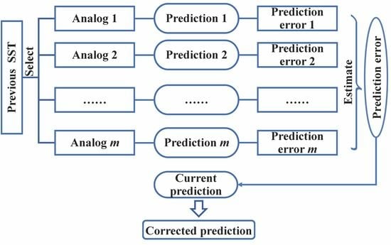
2.3. Analog-Based Correction Method

A brief overview of the ABC method [60,63] is given here:

$$\widehat{\mathrm{Pred}}({\psi }_0)=\mathrm{Pred}({\psi }_0)+\sum _{i=1}^n{w}_i\left[\mathrm{Obs}\left({\tilde{\psi }}_i\right)-\mathrm{Pred}\left({\tilde{\psi }}_i\right)\right]$$

(1)

where $\mathrm{Pred}$ and $\mathrm{Obs}$ refer to model predictions and observations, respectively. In the equation, $w_i$ is the weight function. “$\stackrel{~}{}$” represents the historical analog time. ${\psi }_0$ indicates the current initial state and ${\tilde{\psi }}_i$ is the analogy initial state (i = 1, 2 … n, where n denotes the overall number of analogs chosen). For different ${\psi }_0$, one can target the historical analog ${\tilde{\psi }}_i$ $\mathrm{t}\mathrm{h}\mathrm{a}\mathrm{t}$ is well suited for an estimation of current errors. $\widehat{\mathrm{Pred}}({\psi }_0)$ represents the corrected model prediction. To the right, the first term corresponds to the original model prediction, while the second term represents the prediction correction. The prediction correction term is determined by utilizing historical analog prediction errors from the same model. Furthermore, it should be noted that prediction objectives are expressed in the equation as functions Pred($\psi$) rather than prediction variables $\psi$, indicating that the method can be used to correct either prediction variables (such as geopotential height) or their functions (such as precipitation). Particularly, in this study, the variable $\psi$ denotes SST and $\mathrm{Obs}\left({\tilde{\psi }}_i\right)$ denotes the observed precipitation corresponding to the predicted precipitation $\mathrm{Pred}\left({\tilde{\psi }}_i\right)$ for the initial value ${\tilde{\psi }}_i$.

2.4. Evaluation Methods

The Temporal Correlation Coefficient (TCC) and the Pattern Correlation Coefficient (PCC) are used to quantify model predictability. We define $x_{l,k}$ and $f_{l,k}$ as the anomalies for observation and prediction in space ($l$) and time ($k$); P is the number of space samples; and Q is the number of time samples. They are calculated as follows:

$${\mathrm{TCC}}_l=\frac{{\sum }_{k=1}^Q(x_{l,k}-\overline{x_l})(f_{l,k}-\overline{f_l})}{\sqrt{{\sum }_{k=1}^Q(x_{l,k}-\overline{x_l}{)}^2}\times \sqrt{{\sum }_{k=1}^Q(f_{l,k}-\overline{f_l}{)}^2}},$$

(2)

$${\mathrm{PCC}}_k=\frac{{\sum }_{l=1}^P(x_{l,k}-\overline{x_k})(f_{l,k}-\overline{f_k})}{\sqrt{{\sum }_{l=1}^P(x_{l,k}-\overline{x_k}{)}^2}\times \sqrt{{\sum }_{l=1}^P(f_{l,k}-\overline{f_k}{)}^2}}$$

(3)

The range of the TCC and PCC are from −1.0 to 1.0, and a large positive (negative) value indicates a highly similar (opposite) correlation between prediction and observation.

3. Results

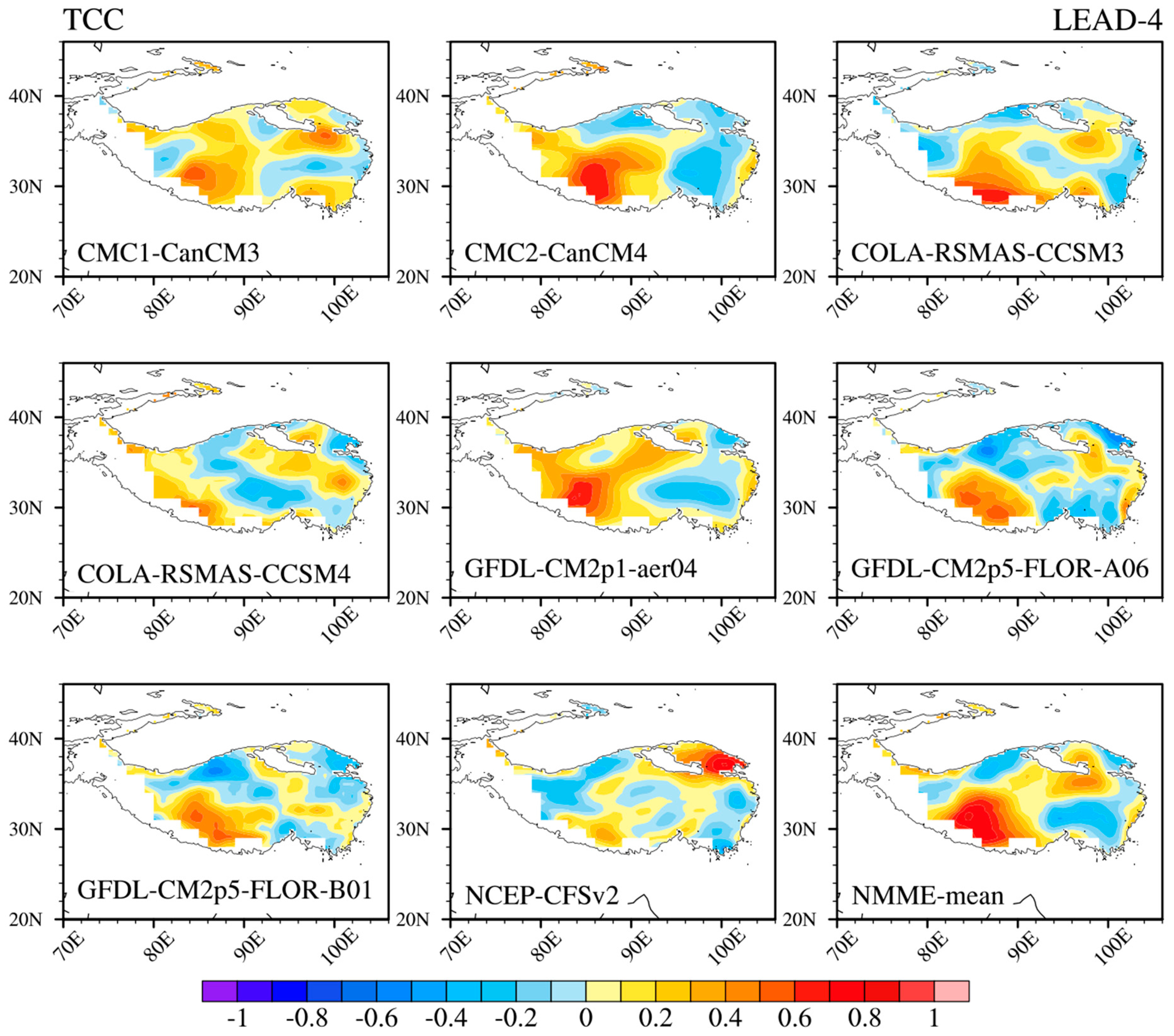
3.1. Evaluation of Model Direct Predictions

Figure 1 shows the TCC skills directly from the individual NMME models, as well as their mean for predicting the TPSP. The individual models exhibit low prediction skills, characterized by significant correlation coefficients limited to small areas in the southwestern TP. The NMME-mean shows higher positive TCC skills, although this improvement is mainly observed in the southwestern TP. The central–eastern TP is characterized by high population density and extensive economic and agricultural activities, indicating the urgent need for improvements in predicting precipitation over this region. The subsequent analysis focuses on identifying effective predictors of TPSP. Next, a new analog-based correction method of dynamical models is developed, utilizing potential predictors.

3.2. The Establishment of the SST Analog-Based Correction Method

Oceanic basin-wide tropical SSTAs have been recognized as critical climate-forcing factors that significantly contribute to climate prediction due to their long-term sustainability with respect to atmospheric processes. Existing studies have extensively examined the oceanic factors that contribute to the inter-annual variability of TPSP, such as ENSO, NAO/AO, and IOBM (e.g., [15,16,17,18,19,21,23]). Specifically, positive anomalies in SST lead to positive anomalies in the upper tropospheric height field and result in anomalous anticyclonic circulation. The SSTAs are modulated by the influence of winter ENSO and Indian Ocean dipole events. Collectively, these oceanic processes regulate the transport of water vapor, subsequently influencing the TPSP [24].

Figure 2 provides the 5-year-out running correlation between the previous February global SSTAs and the TP area-averaged summer precipitation. The delayed influence of the SST was investigated first, with an analysis of the correlation from the TP-averaged precipitation to global SSTAs in February from 1982 to 2018 (shown in Figure 2a). The previous February SSTAs in the Indian Ocean (IO) and North Atlantic Ocean (ATL) were found to be significantly related to the TPSP. The maximum correlation coefficients with the TP-averaged precipitation index are 0.53 and 0.55, respectively. It is essential to recognize that the relationship between two climate systems can exhibit temporal instability, limiting climate predictability (e.g., [75,76,77,78,79]). Taking these considerations into account, further analysis of running correlation coefficients was conducted to determine the optimal predictor domains. These coefficients were evaluated by consecutively excluding 5 years at a time from the time series and calculating correlations between the predictor and precipitation for each omission; a series of correlation values was obtained. The minimal running correlations refer to the reliability of the predictor–precipitation relationship, as illustrated in Figure 2b. Accordingly, the SSTAs identified by the red boxes in Figure 2b were chosen as predictors and labeled as the ATL-SST and IO-SST.

Figure 3 further provides the correlation between the observational region-averaged SST indices in the two key regions (hereafter referred to as IO-index and ATL-index) and the precipitation prediction errors in each individual model [55]. Positive correlations can be found throughout the TP, with the ATL-index demonstrating relatively higher correlation coefficients compared to the IO-index. Moreover, the spatial distributions of correlation coefficients generally exhibit a high degree of similarity among these model results, with the majority of PCCs between SST-TP precipitation correlations for the NMME-mean and individual models exceeding 0.8 (Figure 4). These findings imply that SSTAs within the key regions influence the formation and development of prediction errors, providing insights into prediction error spatial distribution and variability.

In some cases, there may not be available historical years that are directly comparable or considered the “most analogous” to the current year. To address this issue, a flexible approach has been adopted for the final predictions, which involves selecting analog states by evaluating the PCCs that capture the similarity between present and historical SSTAs within the predictor domain, with a threshold set at 0.7. When the correlation between the SSTAs within the predictor domain exceeds 0.7, the corrected precipitation is utilized as the ultimate prediction result. Conversely, when the correlation is less than 0.7, the original model-predicted precipitation is used as the ultimate prediction for that year. This allows for adaptability in capturing the influence of both high and low correlations between the SSTAs in the predictor domain and prediction errors, resulting in more reliable predictions. Based on the aforementioned analysis, two predictors were selected. Consequently, the final predictions are determined by averaging the results of these two selected predictors, referred to as ensemble–mean (EM) predictions.

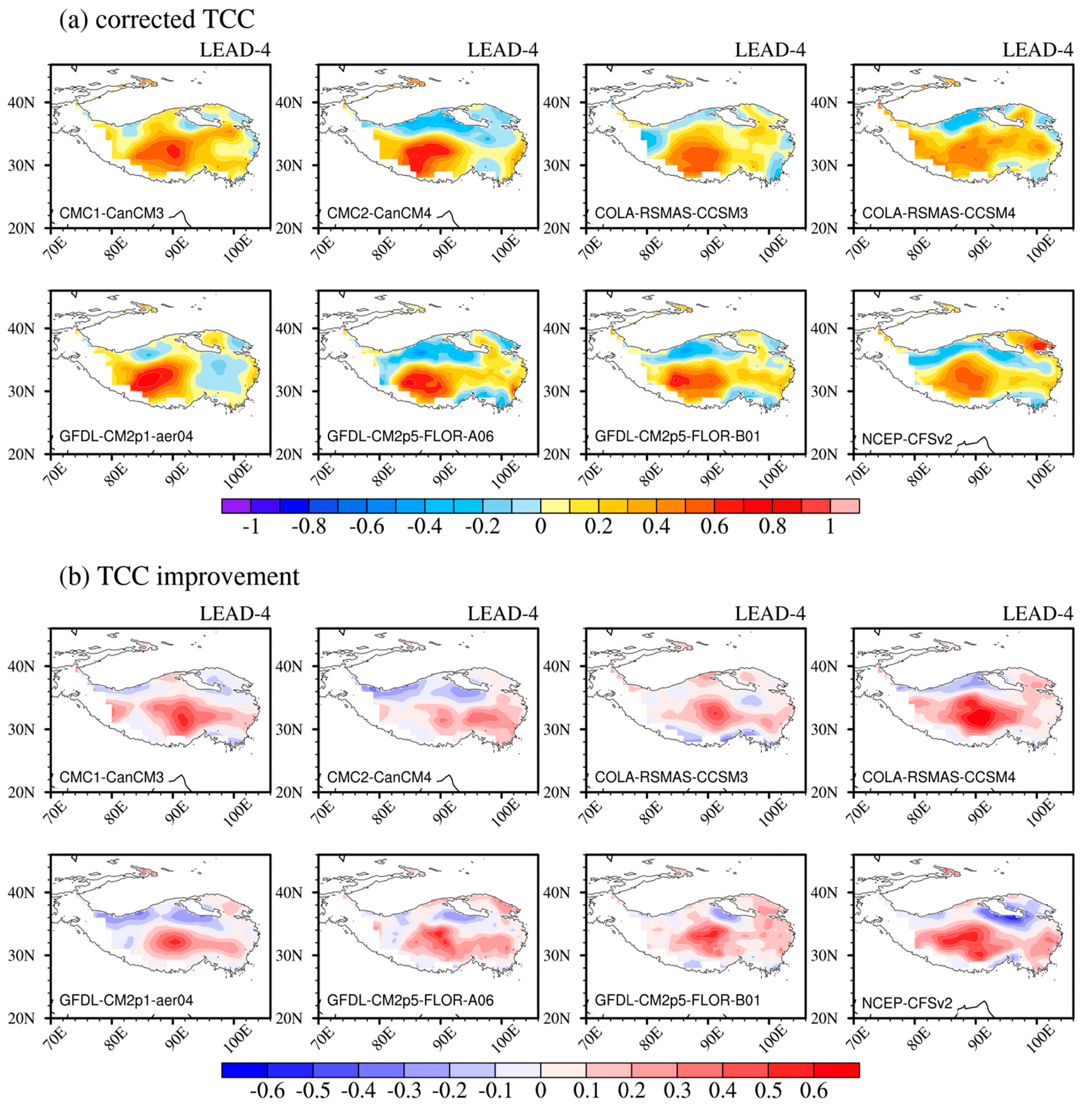
3.3. Validation of the New Method

To validate the new method, rolling-independent reforecast experiments were adopted in this study. This approach involves using only historical observational data from previous years to be utilized for training. For example, for the year 1992 (1993), only observational data from 1982 to 1991 (1982–1992) are utilized to train the model, and so on. Subsequently, a combined dataset spanning from 1992 to 2018, incorporating both hindcasts and operational predictions, is employed for evaluating how well the correction method performs.

Figure 5 and Figure 6 depict the TCC skills of the individual models for JJA mean precipitation after applying the new method, using the predictors of the IO-SST and the ATL-SST, during the rolling-independent period from 1992 to 2018. In comparison to the original predictions, which demonstrate low prediction skill over the central–eastern TP (Figure 1), the new method predictions exhibit significantly improved skill in predicting JJA precipitation. Figure 5b and Figure 6b show the TCC differences between the corrected and the original predictions, highlighting the substantial improvements achieved by the new method in predicting the TPSP. For the corrected predictions of the IO-SST as a predictor, positive values are found throughout the central–eastern TP regions in most models with the highest TCC improvement (over 0.5). When the ATL-SST is used as a predictor, the COLA-RSMAS-CCSM4 model demonstrates the most significant improvement in TCC with a maximum value of 0.81, while the majority of other models also exhibit improvements exceeding 0.5. Using ATL-SST as a predictor leads to a skill improvement, notably in the southwestern TP region in Figure 6, even if the original models already show remarkable skill in this area. This finding is further supported by the skills of area-averaged TCC for both the original and corrected NMME-mean, as shown in Figure S1. Additionally, it can be observed from Figure S1 that the EM predictions combining the two predictors are generally superior to those of each individual predictor alone.

Figure 7 illustrates the spatial patterns of the TCCs of the corrected NMME-mean, as well as the differences between the corrected NMME-mean and the original NMME-mean, for each lead month ranging from 1 to 4. In contrast to the limited improvement observed in the southwestern TP of the original NMME-mean, the corrected NMME-mean exhibits widespread positive TCCs across almost the whole TP region, except for some northern peripheral areas. As seen in Figure 7b, TCCs have significantly improved, with values exceeding 0.6.

Figure 8 presents the PCCs from the observed anomalous precipitation with respect to the predictions generated by both the original NMME-mean and the new method. In most years, the NMME-mean based on the new method exhibits larger or very similar PCCs compared to the original NMME-mean. The long-term averaged PCCs over 1992–2018 increased from approximately 0.16 (0.17, 0.20, and 0.16) of the uncorrected NMME-mean to approximately 0.25 (0.23, 0.27, and 0.28) of the original NMME-mean at lead time of one month (two months, three months, and four months). Figure S2 shows substantial improvements in the long-term averaged PCCs for the individual models derived from the new method. The results obtained from this study indicate that the new method has the ability to significantly improve the prediction of the TPSP.

4. Discussion

The TP poses considerable challenges for accurately predicting summer precipitation due to its unique geographical features, complex topography, and atmospheric circulation patterns. Current dynamical models have limitations in accurately capturing TPSP. This study introduces a new analog-based correction method that has been developed to address this challenge and improve the prediction of the TPSP. The method is motivated by the hypothesis that the flow-dependent model prediction errors exhibit some degree of similarity when the prior climate states of the models are analogous to one another. When the new method is applied to the NMME model hindcasts dataset, the verification against independent observations shows that the new SST analog-based correction method of dynamical models can evidently improve prediction skills of summer precipitation in most TP regions.

Over the past few years, dynamic models have become the most powerful tool in climate predictions. However, it is inevitable that these models will have inherent errors in their predictions. Specifically, prediction errors refer to the disparities between the predicted values and the corresponding observed values. The errors are known to vary with the climate state, which can be estimated statistically using related physical variables as predictors. In other words, the variability of the climate system directly or indirectly influences the configuration and evolution of prediction errors, and such influences will further be reflected in the distribution and change in prediction errors. This serves as the fundamental premise of the present study. Our study examined the correlation between preceding February SSTAs and prediction errors of TPSP. The analysis reveals a significant relationship between prediction errors and preceding February SSTAs in key regions of the Indian Ocean and North Atlantic Ocean. Additionally, a high degree of similarity in the prediction errors is observed among different dynamical models utilized in this study. In simpler terms, when the SSTAs in February exhibit similarities, it is possible for the model prediction errors to exhibit similar patterns as well. This formed the basis of our method, and we utilized this relationship to estimate error weights by combining them. Building on these findings, the analog-based correction method has been applied to predict summer precipitation using the identified SST predictors. The rolling-independent validation technique has been used from 1992 to 2018 to verify the new method. The findings of this study demonstrate promising results for the proposed correction method in predicting summer precipitation over the TP. Both the IO-SST and ATL-SST exhibit superior performance with positive TCCs over most areas of the TP, albeit with regional differences. The EM predictions using both the IO-SST and ATL-SST predictors demonstrate superior performance compared to each predictor individually. This approach provided a novel perspective and practical application for error correction in climate prediction, ultimately contributing to the advancement of the field.

Our findings provided insights that, despite the overall positive performance exhibited by the IO-SST and ATL-SST, there are regional differences indicating that individual predictors may exert specific influences on particular areas of the TP. The regional variations could be attributed to the complex interactions between atmospheric and oceanic processes, as well as the specific geographical features and atmospheric circulation patterns in different sub-regions of the TP. Therefore, future prediction research will consider dividing the entire TP into several sub-regions. In addition to our focus on SST predictors, previous studies, as mentioned in our introduction, have extensively investigated the influence of ENSO on TP precipitation. We also explored the application of an ENSO-based ABC method to predict TP summer precipitation. However, despite our efforts, this approach has not yielded a significant improvement in prediction skills. Notably, Liu and Ren (2023) found that EP El Niño and CP La Niña have contrasting effects on summer precipitation in the southwestern TP, resulting in a trans-type inversion characterized by significant decreases and increases, respectively [19]. These findings highlight the complexity of the relationship between ENSO and TP precipitation, which is may also reflected in model errors. Considering the intricate nature of this relationship, our future investigations aim to delve deeper into the characteristics of TP precipitation under different ENSO event types and apply the findings to improve the TPSP prediction in dynamical models. Beyond that, it is possible to consider that nonlinear prediction errors can be objectively isolated and addressed via alternative nonlinear methodologies, including deep learning techniques [80].

Although the new method for TP precipitation shows significant improvement, it is important to acknowledge that its performance may vary across different time periods. The variation can arise from uncertainties between the predictor and predictand at interdecadal or decadal scales [81]. Therefore, achieving stable and highly skilled TP precipitation prediction remains a major challenge. In this study, the analog-based correction mechanism is exclusively established using the preceding SST signals. Nevertheless, it is imperative to acknowledge the intricate and extensive drivers of TPSP variability. Other boundary signals, including snow cover and soil moisture [82,83,84,85], may also influence TPSP. In addition, we used bilinear interpolation to estimate the values at the grid points in the interpolated dataset. It is also important to acknowledge the limitations and potential biases associated with interpolation techniques. Bilinear interpolation assumes a uniform distribution of data in space and equal distances between grid points. In reality, there may be discrepancies in spatial resolution or grid layout between the observed datasets and the model data, which could introduce interpolation bias. Although it is not possible to eliminate this type of bias entirely, in order to improve the reliability of the observational data, we employed multiple datasets. This ensemble averaging approach involved calculating the mean value across the three datasets at each grid point, resulting in a composite precipitation dataset. This helped to reduce the impact of individual dataset biases and improve the representativeness of the interpolated dataset. In addition, in our study, we also compared the skills verified by directly using each set of observational data, respectively. It is evident that the overall distribution of TCC skills remains relatively consistent. These findings align with the results obtained from multiple observational ensembles. Despite the inherent variability in the observation data, we made diligent efforts to account for its influence, and via comprehensive analysis, we demonstrated the robustness of our error correction method from multiple perspectives.

5. Conclusions

This study introduced an analog-based correction method aimed at improving summer precipitation prediction over the TP. The new method has been successfully applied to predict precipitation for the models included in the NMME dataset. The performance of the new method is validated by utilizing remote-sensing-based and observational datasets as benchmarks. Three main conclusions were obtained as follows:

(1)

The prediction skill for summer precipitation over the TP in current climate models is constrained, with notable limitations observed in the central–eastern TP region. Additionally, the prediction errors demonstrate a pronounced level of consistency across various dynamical models.

(2)

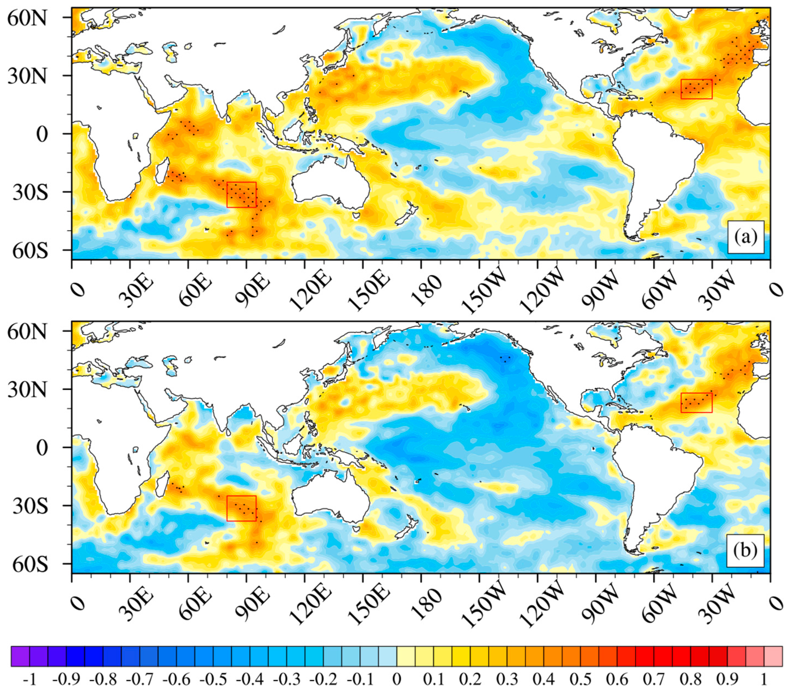
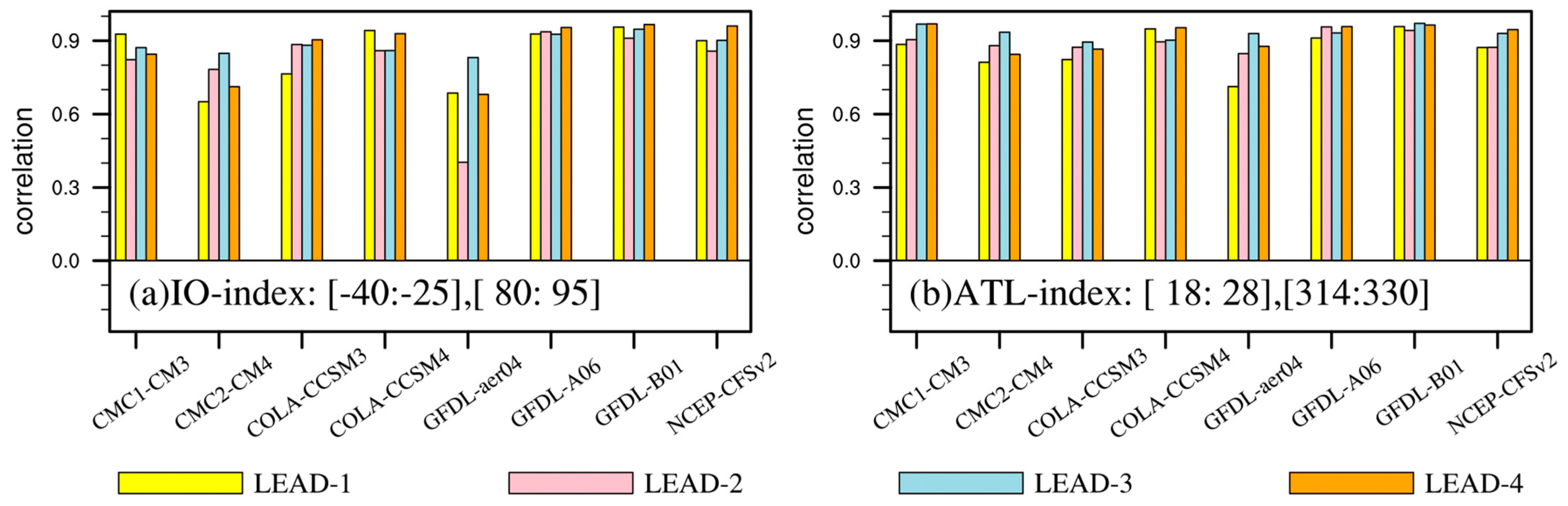
The prediction errors of TPSP exhibit a significant correlation with the previous February anomalies of SST in the key regions of the tropical Ocean. Both the ATL-SST and IO-SST can be considered effective predictors for correcting the prediction errors while noting the presence of regional differences.

(3)

The prediction skill for summer precipitation over the TP exhibits notable improvements via the application of the new SST analog-based correction method, as demonstrated by higher temporal and spatial skill scores obtained from the rolling-independent verification. This study provides a valuable tool for enhancing the prediction of TPSP within dynamical models.

References

1. Qiu, J. China: The third pole. Nature 2008, 454, 393–396. [Google Scholar] [CrossRef]
2. Yao, T.; Xue, Y.; Chen, D.; Chen, F.; Thompson, L.; Cui, P.; Koike, T.; Lau, W.K.-M.; Lettenmaier, D.; Mosbrugger, V.; et al. Recent Third Pole’s Rapid Warming Accompanies Cryospheric Melt and Water Cycle Intensification and Interactions between Monsoon and Environment: Multidisciplinary Approach with Observations, Modeling, and Analysis. Bull. Am. Meteorol. Soc. 2019, 100, 423–444. [Google Scholar] [CrossRef]
3. Nowak, A.S.; Nobis, M. Distribution patterns, floristic structure and habitat requirements of the alpine river plant community Stuckenietum amblyphyllae ass. nova (Potametea) in the Pamir Alai Mountains (Tajikistan). Acta Soc. Bot. Pol. 2012, 81, 101–108. [Google Scholar] [CrossRef]
4. Sun, J.; Cheng, G.; Li, W.; Sha, Y.; Yang, Y. On the Variation of NDVI with the Principal Climatic Elements in the Tibetan Plateau. Remote Sens. 2013, 5, 1894–1911. [Google Scholar] [CrossRef]
5. Immerzeel, W.W.; van Beek, L.P.; Bierkens, M.F. Climate change will affect the Asian water towers. Science 2010, 328, 382–1385. [Google Scholar] [CrossRef]
6. Flohn, H. Large-scale aspects of the ‘summer monsoon’ in South and East Asia. J. Meteorol. Soc. Jpn. 1957, 75, 180–186. [Google Scholar] [CrossRef]
7. Yeh, T.C.; Lo, S.W.; Chu, P.C. On the heat balance and circulation structure in troposphere over Tibetan Plateau. Acta Meteorol. Sin. 1957, 28, 108–121. (In Chinese) [Google Scholar]
8. Ueda, H.; Kamahori, H.; Yamazaki, N. Seasonal contrasting features of heat and moisture budgets between the eastern and western Tibetan plateau during the GAME IOP. J. Clim. 2003, 16, 2309–2324. [Google Scholar] [CrossRef]
9. Bibi, S.; Wang, L.; Li, X.; Zhou, J.; Chen, D.; Yao, T. Climatic and associated cryospheric, biospheric, and hydrological changes on the Tibetan Plateau: A review. Int. J. Climatol. 2018, 38, e1–e17. [Google Scholar] [CrossRef]
10. Dong, W.; Lin, Y.; Wright, J.S.; Ming, Y.; Xie, Y.; Wang, B.; Luo, Y.; Huang, W.; Huang, J.; Wang, L.; et al. Summer rainfall over the southwestern Tibetan Plateau controlled by deep convection over the Indian subcontinent. Nat. Commun. 2016, 7, 10925. [Google Scholar] [CrossRef] [PubMed]
11. Yao, T.; Thompson, L.; Yang, W.; Yu, W.-S.; Gao, Y.; Guo, X.-J.; Yang, X.; Duan, K.; Zhao, H.; Xu, B.; et al. Different glacier status with atmospheric circulations in Tibetan Plateau and surroundings. Nat. Clim. Chang. 2012, 2, 663–667. [Google Scholar] [CrossRef]
12. Duan, A.; Wu, G. Weakening trend in the atmospheric heat source over the Tibetan Plateau during recent decades. Part I: Observations. J. Clim. 2008, 21, 3149–3164. [Google Scholar] [CrossRef]
13. Wu, Z.; Li, J.; Jiang, Z.; Ma, T. Modulation of the Tibetan Plateau Snow Cover on the ENSO Teleconnections: From the East Asian Summer Monsoon Perspective. J. Clim. 2012, 25, 2481–2489. [Google Scholar] [CrossRef]
14. Jiang, X.; Li, Y.; Yang, S.; Yang, K.; Chen, J. Interannual Variation of Summer Atmospheric Heat Source over the Tibetan Plateau and the Role of Convection around the Western Maritime Continent. J. Clim. 2016, 29, 121–138. [Google Scholar] [CrossRef]
15. Gao, X.; Wang, M.; Filippo, G. Climate Change over China in the 21st Century as Simulated by BCC_CSM1.1-RegCM4.0. Atmos. Ocean. Sci. Lett. 2013, 6, 381–386. [Google Scholar]
16. Wang, C.; Ma, Z. Quasi-3-yr cycle of rainy season precipitation in Tibet related to different types of ENSO during 1981–2015. J. Meteorol. Res. 2018, 32, 181–190. [Google Scholar] [CrossRef]
17. Hu, S.; Zhou, T.; Wu, B. Impact of Developing ENSO on Tibetan Plateau Summer Rainfall. J. Clim. 2021, 34, 3385–3400. [Google Scholar] [CrossRef]
18. Hu, S.; Wu, B.; Zhou, T.; Yu, Y. Dominant Anomalous Circulation Patterns of Tibetan Plateau Summer Climate Generated by ENSO-Forced and ENSO-Independent Teleconnections. J. Clim. 2022, 35, 1679–1694. [Google Scholar] [CrossRef]
19. Liu, M.; Ren, H.-L.; Wang, R.; Ma, J.; Mao, X. Distinct Impacts of Two Types of Developing El Niño–Southern Oscillations on Tibetan Plateau Summer Precipitation. Remote Sens. 2023, 15, 4030. [Google Scholar] [CrossRef]
20. Yang, X.; Yao, T.; Deji; Zhao, H.; Xu, B. Possible ENSO Influences on the Northwestern Tibetan Plateau Revealed by Annually Resolved Ice Core Records. J. Geophys. Res. Atmos. 2018, 123, 3857–3870. [Google Scholar] [CrossRef]
21. Chen, X.; You, Q. Effect of Indian Ocean SST on Tibetan Plateau Precipitation in the Early Rainy Season. J. Clim. 2017, 30, 8973–8985. [Google Scholar] [CrossRef]
22. Zhao, Y.; Duan, A.; Wu, G. Interannual variability of late-spring circulation and diabatic heating over the Tibetan Plateau associated with Indian Ocean forcing. Adv. Atmos. Sci. 2018, 35, 927–941. [Google Scholar] [CrossRef]
23. Liu, X.; Yin, Z. Spatial and Temporal Variation of Summer Precipitation over the Eastern Tibetan Plateau and the North Atlantic Oscillation. J. Clim. 2001, 14, 2896–2909. [Google Scholar] [CrossRef]
24. He, K.; Liu, G.; Wu, R.; Nan, S.; Wang, S.; Zhou, C.; Qi, D.; Mao, X.; Wang, H.; Wei, X. Oceanic and land relay effects in the link between spring sea surface temperatures in the Indian Ocean and summer precipitation over the Tibetan Plateau. Atmos. Res. 2022, 266, 105953. [Google Scholar] [CrossRef]
25. Wang, Z.; Duan, A.; Yang, S.; Ullah, K. Atmospheric moisture budget and its regulation on the variability of summer precipitation over the Tibetan Plateau. J. Geophys. Res. Atmos. 2017, 122, 614–630. [Google Scholar] [CrossRef]
26. Wang, B.; Lee, J.-Y.; Kang, I.-S.; Shukla, J.; Park, C.K.; Kumar, A.; Schemm, J.; Cocke, S.; Kug, J.-S.; Luo, J.-J.; et al. Advance and prospectus of seasonal prediction: Assessment of the APCC/ CliPAS 14-model ensemble retrospective seasonal prediction (1980–2004). Clim. Dyn. 2009, 33, 93–117. [Google Scholar] [CrossRef]
27. Wang, B.; Lee, J.-Y.; Xiang, B. Asian summer monsoon rainfall predictability: A predictable mode analysis. Clim. Dyn. 2015, 44, 61–74. [Google Scholar] [CrossRef]
28. Yu, R.; Li, J.; Zhang, Y.; Chen, H. Improvement of rainfall simulation on the steep edge of the Tibetan Plateau by using a finite-difference transport scheme in CAM5. Clim. Dyn. 2015, 45, 2937–2948. [Google Scholar] [CrossRef]
29. Bao, Q.; Wu, X.; Li, J.; Wang, L.; He, B.; Wang, X.; Liu, Y.; Wu, G. Outlook for El Niño and the Indian Ocean Dipole in autumn-winter 2018–2019. Chin. Sci. Bull. 2019, 64, 73–78. [Google Scholar] [CrossRef]
30. Bao, Q.; Li, J. Progress in climate modeling of precipitation over the Tibetan Plateau. Natl. Sci. Rev. 2020, 7, 486–487. [Google Scholar] [CrossRef]
31. He, B.; Bao, Q.; Wang, X.; Zhou, L.; Wu, X.; Liu, Y.; Wu, G.; Chen, K.; He, S.; Hu, W.; et al. CAS FGOALS-f3-L Model Datasets for CMIP6 Historical Atmospheric Model Intercomparison Project Simulation. Adv. Atmos. Sci. 2019, 36, 771–778. [Google Scholar] [CrossRef]
32. Lee, W.L.; Liou, K.N.; Wang, C. Impact of 3-D topography on surface radiation budget over the Tibetan Plateau. Theor. Appl. Climatol. 2013, 113, 95–103. [Google Scholar] [CrossRef]
33. Wang, L.; Ren, H.-L.; Xu, X.; Huang, B.; Wu, J.; Liu, J. Seasonal-interannual predictions of summer precipitation over the Tibetan Plateau in North American Multimodel Ensemble. Geophys. Res. Lett. 2022, 49, e2022GL100294. [Google Scholar] [CrossRef]
34. Palmer, T.; Alessandri, A.; Andersen, U.; Cantelaube, P.; Davey, M.; Délécluse, P.; Déqué, M.; Díez, E.; Doblas-Reyes, F.J.; Feddersen, H.; et al. Development of a European multimodel ensemble system for seasonal to interannual prediction (DEMETER). Bull. Am. Meteorol. Soc. 2004, 85, 853–872. [Google Scholar] [CrossRef]
35. Hewitt, C.D.; Griggs, D.J. Ensembles-based predictions of climate change and their impacts (ENSEMBLES). EOS Trans. AGU 2004, 85, 566. [Google Scholar]
36. Kirtman, B.P.; Min, D.; Infanti, J.M.; Kinter, J.L.; Paolino, D.A.; Zhang, Q.; van den Dool, H.; Saha, S.; Mendez, M.; Becker, E.; et al. Phase-1 seasonal to interannual prediction, phase-2 toward developing intra-seasonal prediction. Bull. Am. Meteorol. Soc. 2014, 95, 585–601. [Google Scholar] [CrossRef]
37. Shukla, S.; Jason, R.; Hoell, A.; Funk, C.; Franklin, R.C.; Kirtman, B. Assessing North American multimodel ensemble (NMME) seasonal forecast skill to assist in the early warning of anomalous hydrometeorological events over East Africa. Clim. Dyn. 2019, 53, 7411–7427. [Google Scholar] [CrossRef]
38. Slater, L.J.; Villarini, G.; Bradley, A.A. Weighting of NMME temperature and precipitation forecasts across Europe. J. Hydrol. 2017, 552, 646–659. [Google Scholar] [CrossRef]
39. Giannini, A.; Ali, A.; Kelley, C.P.; Lamptey, B.L.; Minoungou, B.; Ndiaye, O. Advances in the lead time of Sahel rainfall prediction with the North American Multimodel Ensemble. Geophys. Res. Lett. 2020, 47, e2020GL087341. [Google Scholar] [CrossRef]
40. Ren, H.L.; Wu, Y.J.; Bao, Q.; Ma, J.H.; Li, Q.P.; Wan, J.H.; Li, Q.; Wu, X.; Liu, Y.; Tian, B.; et al. China multi-model ensemble prediction system version 1.0 (CMMEv1.0) and its application to flood-season prediction in 2018. J. Meteorol. Res. 2019, 31, 542–554. [Google Scholar]
41. Wigley, T.M.L.; Jones, P.D.; Briffa, K.R.; Smith, G. Obtaining sub-grid-scale information from coarse-resolution general circulation model output. J. Geophys. Res. Atmos. 1990, 95, 1943–1953. [Google Scholar] [CrossRef]
42. Zeng, Q.C.; Zhang, B.L.; Yuan, C.G.; Lu, P.S.; Yang, F.L.; Li, X.; Wang, H.J. A note on some methods suitable for verifying and correcting the prediction of climate anomaly. Adv. Atmos. Sci. 1994, 11, 121–127. [Google Scholar]
43. Zeng, Q.C.; Yuan, C.G.; Xu, L.; Zhang, R.H.; Yang, F.L.; Zhang, B.L.; Lu, P.S.; Bi, X.Q.; Wang, H.J. Seasonal and Extraseasonal predictions of summer monsoon precipitation by GCMs. Adv. Atmos. Sci. 1997, 14, 163–176. [Google Scholar]
44. Busuioc, A.; Von Storch, H.; Schnur, R. Verification of GCM-generated regional seasonal precipitation for current climate and of statistical downscaling estimates under changing climate conditions. J. Clim. 1999, 12, 258–272. [Google Scholar] [CrossRef]
45. Wang, H.J.; Fan, K. A New Scheme for Improving the Seasonal Prediction of Summer Precipitation Anomalies. Wea. Forecast. 2009, 24, 548–554. [Google Scholar] [CrossRef]
46. Liu, Y.; Fan, K. An application of hybrid downscaling model to forecast summer precipitation at stations in China. Atmos. Res. 2014, 143, 17–30. [Google Scholar] [CrossRef]
47. Yu, H.P.; Zhang, Q.; Wei, Y.; Liu, C.X.; Ren, Y.; Yue, P.; Zhou, J. Bias-corrections on aridity index simulations of climate models by observational constraints. Int. J. Climatol. 2022, 42, 889–907. [Google Scholar] [CrossRef]
48. Wu, J.; Ren, H.L.; Zhang, P.; Wang, Y.; Liu, Y.; Zhao, C.; Li, Q. The dynamical-statistical subseasonal prediction of precipitation over China based on the BCC new-generation coupled model. Clim. Dyn. 2022, 59, 1213–1232. [Google Scholar] [CrossRef]
49. Ma, J.H.; Sun, J.Q. New statistical prediction scheme for monthly precipitation variability in the rainy season over northeastern China. Int. J. Climatol. 2021, 41, 5805–5819. [Google Scholar] [CrossRef]
50. Ma, J.H.; Sun, J.Q.; Liu, C.Z. A hybrid statistical-dynamical prediction scheme for summer monthly precipitation over Northeast China. Meteorol. Appl. 2022, 29, e2057. [Google Scholar] [CrossRef]
51. Zhu, Y.; Sun, J.; Ma, J. A hybrid statistical-dynamical prediction model for summer precipitation in northwestern China based on NCEP CFSv2. Atmos. Res. 2023, 283, 106567. [Google Scholar] [CrossRef]
52. Ren, H.-L. Predictor-based error correction method in short-term climate prediction. Prog. Nat. Sci. 2008, 18, 129–135. [Google Scholar] [CrossRef]
53. Yang, X.Q.; Anderson, J.L. Correction of systematic errors in coupled GCM forecasts. J. Clim. 2000, 13, 2072–2085. [Google Scholar] [CrossRef]
54. Gu, W.; Chen, L.; Li, W.; Chen, D. Development of a downscaling method in China regional summer precipitation prediction. Acta Meteorol. Sin. 2011, 25, 303–315. [Google Scholar] [CrossRef]
55. Samadi, S.; Wilson, C.A.; Moradkhani, H. Uncertainty analysis of statistical downscaling models using Hadley centre coupled model. Theor. Appl. Climatol. 2013, 4, 673–690. [Google Scholar] [CrossRef]
56. Paul, S.; Liu, C.M.; Chen, J.M.; Lin, S.H. Development of a statistical downscaling model for projecting monthly rainfall over East Asia from a general circulation model output. J. Geophys. Res. Atmos. 2008, 113, D15117. [Google Scholar] [CrossRef]
57. Fan, K.; Wang, H.J.; Choi, Y.-J. A physically-based statistical forecast model for the middle-lower reaches of the Yangtze River Valley summer rainfall. Chin. Sci. Bull. 2008, 53, 602–609. [Google Scholar] [CrossRef]
58. Fan, K.; Liu, Y.; Chen, H.P. Improving the prediction of the East Asian summer monsoon: New approaches. Wea. Forecast. 2012, 27, 1017–1030. (In Chinese) [Google Scholar] [CrossRef]
59. Ren, H.-L.; Chou, J.F. Analog correction method of errors by combining statistical and dynamical methods. Acta Meteorol. Sin. 2006, 20, 367–373. [Google Scholar]
60. Ren, H.-L.; Chou, J.F. Strategy and methodology of dynamical analogue prediction. Sci. China Ser. D Earth Sci. 2007, 50, 1589–1599. [Google Scholar] [CrossRef]
61. Ren, H.-L.; Chou, J.F.; Huang, J.P.; Zhang, P. Theoretical basis and application of analogue-dynamical model in the Lorenz system. Adv. Atmos. Sci. 2009, 26, 67–77. [Google Scholar] [CrossRef]
62. Yu, H.P.; Huang, J.P.; Chou, J.F. Improvement of Medium-Range Forecasts Using the Analog-Dynamical Method. Mon. Wea. Rev. 2014, 142, 1570–1587. [Google Scholar] [CrossRef]
63. Ren, H.-L.; Liu, Y.; Jin, F.-F.; Yan, Y.P.; Liu, X.W. Application of the analogue-based correction of errors method in ENSO prediction. Atmos. Ocean. Sci. Lett. 2014, 7, 157–161. [Google Scholar]
64. Liu, Y.; Ren, H.-L. Improving ENSO prediction in CFSv2 with an analogue-based correction method. Int. J. Climatol. 2017, 37, 5035–5046. [Google Scholar] [CrossRef]
65. Becker, E.; den Dool, H.V.; Zhang, Q. Predictability and Forecast Skill in NMME. J. Clim. 2014, 27, 5891–5906. [Google Scholar] [CrossRef]
66. Becker, E.; Kirtman, B.P.; Pegion, K. Evolution of the North American multi-model ensemble. Geophys. Res. Lett. 2020, 47, e2020GL087408. [Google Scholar] [CrossRef]
67. Merryfield, W.J.; Lee, W.S.; Boer, G.J.; Kharin, V.V.; Scinocca, J.F.; Flato, G.M.; Ajayamohan, R.S.; Fyfe, J.C.; Tang, Y.; Polavarapu, S. The Canadian Seasonal to Interannual Prediction System. Part I: Models and initialization. Mon. Weather Rev. 2013, 141, 2910–2945. [Google Scholar] [CrossRef]
68. Kirtman, B.P.; Min, D. Multimodel Ensemble ENSO Prediction with CCSM and CFS. Mon. Weather Rev. 2009, 137, 2908–2930. [Google Scholar] [CrossRef]
69. Infanti, J.; Kirtman, B. Southeastern US Rainfall Prediction in the North American Multi-Model Ensemble. J. Hydrol. 2014, 15, 529–550. [Google Scholar]
70. Vecchi, G.A.; Delworth, T.; Gudgel, R.; Kapnick, S.; Rosati, A.; Wittenberg, A.T.; Zeng, F.; Anderson, W.; Balaji, V.; Dixon, K.; et al. On the Seasonal Forecasting of Regional Tropical Cyclone Activity. J. Clim. 2014, 27, 7994–8016. [Google Scholar] [CrossRef]
71. Saha, S.; Moorthi, S.; Wu, X.R.; Wang, J.D.; Nadiga, S.; Tripp, P.; Behringer, D.; Hou, Y.-T.; Chuang, H.-Y.; Iredell, M.; et al. The NCEP Climate Forecast System Version 2. J. Clim. 2014, 27, 2185–2208. [Google Scholar] [CrossRef]
72. Wu, J.; Gao, X. A gridded daily observation dataset over China region and comparison with the other datasets. Chin. J. Geophys. 2013, 56, 1102–1111. (In Chinese) [Google Scholar]
73. Harris, I.C.; Jones, P.D.; Osborn, T. CRU TS4.05: Climatic Research Unit (CRU) Time-Series (TS) Version 4.05 of High-Resolution Gridded Data of Month-by-Month Variation in Climate (Jan. 1901–Dec. 2020); NERC EDS Centre for Environmental Data Analysis: Chicago, IL, USA, 2021. [Google Scholar]
74. Adler, R.F.; Sapiano, M.R.P.; Huffman, G.J.; Wang, J.-J.; Gu, G.; Bolvin, D.; Chiu, L.; Schneider, U.; Becker, A.; Nelkin, E.; et al. The Global Precipitation Climatology Project (GPCP) Monthly Analysis (New Version 2.3) and a Review of 2017 Global Precipitation. Atmosphere 2018, 9, 138. [Google Scholar] [CrossRef]
75. Kumar, K.K.; Rajagopalan, B.; Cane, M.A. On the weakening relationship between the Indian monsoon and ENSO. Science 1999, 284, 2156–2159. [Google Scholar] [CrossRef]
76. Wang, H.J. The instability of the East Asian summer monsoon ENSO relations. Adv. Atmos. Sci. 2002, 19, 1–11. [Google Scholar]
77. Sun, J.Q.; Wang, H.J.; Yuan, W. Decadal variations of the relationship between the summer North Atlantic Oscillation and middle East Asian air temperature. J. Geophys. Res. 2008, 113, D15107. [Google Scholar] [CrossRef]
78. Sun, J.Q.; Wang, H.J.; Yuan, W. Linkage of the boreal spring Antarctic Oscillation to the West African Summer Monsoon. J. Meteorol. Soc. Jpn. 2010, 88, 15–28. [Google Scholar] [CrossRef]
79. Sun, J.Q.; Ahn, B.J. A GCM-based forecasting model for the landfall of tropical cyclones in China. Adv. Atmos. Sci. 2011, 28, 1049–1055. [Google Scholar] [CrossRef]
80. Ham, Y.G.; Kim, J.H.; Luo, J.J. Deep learning for multi-year ENSO forecasts. Nature 2019, 573, 568–572. [Google Scholar] [CrossRef]
81. Wang, B.; Xiang, B.; Li, J.; Webster, P.J.; Rajeevan, M.N.; Liu, J.; Ha, K.-J. Rethinking Indian monsoon rainfall prediction in the context of recent global warming. Nat. Commun. 2015, 6, 7154. [Google Scholar] [CrossRef]
82. Xu, J.J.; Lu, J. Precipitation over the Qinghai-Xizang Plateau in summer and its association with the Eurasian snow cover. J. Nanjing Inst. Meteorol. 1992, 15, 517–524. (In Chinese) [Google Scholar]
83. Wu, B.Y.; Zhang, R.H.; Wang, B.; Rosanne, D.A. On the association between spring Arctic sea ice concentration and Chinese summer rainfall. Geophys. Res. Lett. 2009, 36, L09501. [Google Scholar] [CrossRef]
84. Wu, R.G.; Kirtman, B.P. Observed relationship of spring and summer east Asian rainfall with winter and spring Eurasian snow. J. Clim. 2007, 20, 1285–1304. [Google Scholar] [CrossRef]
85. Yang, S.; Xu, L.Z. Linkage between Eurasian winter snow cover and regional Chinese summer rainfall. Int. J. Climatol. 1994, 14, 739–750. [Google Scholar] [CrossRef]
Figure 1. TCC skills between the observed and predicted TPSP, derived from the original NMME models and NMME-mean at four-month lead during 1992–2018.
Remotesensing 15 05669 g001
Figure 2. (a) The correlation map and (b) the 5-year-out running correlation map between the previous February global SSTAs and the TP area-averaged summer precipitation during the whole period of 1982–2018. The dotted areas denote the statistical significance of Student’s t-test at the 99% confidence level.
Remotesensing 15 05669 g002
Figure 3. The correlation maps between prediction errors of JJA precipitation at a four-month lead and the observed (a) IO-index and (b) ATL-index during the whole period of 1982–2018.
Remotesensing 15 05669 g003
Figure 4. The PCCs between the NMME-mean and individual models for the correlation maps (obtained from Figure 3) of the JJA precipitation prediction errors and the observed (a) IO-index and (b) ATL-index.
Remotesensing 15 05669 g004
Figure 5. (a) Patterns of TCC skills for the new method of the IO-SST as predictor (top 2 rows) and (b) the skill differences between the corrected and original models (bottom 2 rows) at four-month lead during the period of 1992–2018.
Remotesensing 15 05669 g005
Figure 6. (a) Patterns of TCC skills for the new method of the ATL-SST as predictor (top 2 rows) and (b) the skill differences between the corrected and original models (bottom 2 rows) at four-month lead, during the period of 1992–2018.
Remotesensing 15 05669 g006
Figure 7. Patterns of TCC skills (a) for the corrected NMME-mean from the new method of combining two selected predictors and the skill differences (b) between the corrected and original NMME-mean predictions during the period of 1992–2018. The first to fourth rows reflect one- to four-month leads, respectively.
Remotesensing 15 05669 g007
Figure 8. PCCs for the predictions of the original NMME-mean, as well as the corrected NMME-mean from the new method of combining two selected predictors, during the period of 1992–2018. The first to fourth rows reflect one- to four-month leads, respectively. The long-term averaged PCC skills are given in the top-right for each panel.
Remotesensing 15 05669 g008