
Comparative Study of 2D Lattice Boltzmann Models for Simulating Seismic Waves


1
CAS Engineering Laboratory for Deep Resources Equipment and Technology, Institute of Geology and Geophysics, and Innovation Academy for Earth Science, Chinese Academy of Sciences, Beijing 100029, China
2
National Key Laboratory of Petroleum Resources and Engineering, CNPC Key Laboratory of Geophysical Exploration, China University of Petroleum (Beijing), Beijing 102249, China
*
Author to whom correspondence should be addressed.
Remote Sens. 2024, 16(2), 285; https://doi.org/10.3390/rs16020285
Submission received: 6 November 2023
/
Revised: 4 January 2024
/
Accepted: 8 January 2024
/
Published: 10 January 2024
(This article belongs to the Special Issue Recent Advances in Underwater and Terrestrial Remote Sensing)
Abstract
:The simulation of seismic wavefields holds paramount significance in understanding subsurface structures and seismic events. The lattice Boltzmann method (LBM) provides a computational framework adept at capturing detailed wave interactions, offering a new approach to improve seismic wavefield simulations. Our study involves a novel comparative analysis of wavefields using different lattice Boltzmann models, focusing on how relaxation times, discrete velocity models, and collision operators affect simulation accuracy and efficiency. We explore the impacts of distinct relaxation times and evaluate their effects on wave propagation speed and fidelity. By incorporating four discrete velocity models of LBM, we innovatively investigate the trade-off between spatial resolution and computational complexity. Additionally, we delve into the implications of employing three collision operators—single relaxation time (SRT), two relaxation times (TRT), and multiple relaxation times (MRT). By comparing their accuracy and stability, we provide insights into selecting the most suitable collision operator for capturing complex wave interactions. Our research provides a comprehensive framework to optimize the LBM parameters, enhancing both accuracy and efficiency in seismic wave simulations, and offers valuable insights to benefit wave simulation across diverse disciplines.

1. Introduction
Seismic numerical simulation is a crucial research method in seismology, providing valuable insights into the mechanism of earthquakes, seismic event prediction, risk assessment, exploration of the Earth’s internal structure, oil and gas exploration, and resource development. Additionally, seismic modeling forms the foundation for full-waveform inversion [1,2,3,4,5,6,7] and reverse-time migration [8,9,10,11,12,13,14], and aids seismic interpretation.
The lattice Boltzmann method (LBM) is a powerful numerical approach for simulating macroscopic fluid dynamics based on mesoscopic kinetic equations. Its applicability also extends to wavefield simulation. In the past 30 years, researchers have proposed various collision models to broaden the application scope of the LBM. These models comprise the lattice Bhatnagar–Gross–Krook (BGK) model, also known as the single-relaxation-time (SRT) model, as well as the two-relaxation-times (TRT) and multiple-relaxation-times (MRT) collision models. The LBM has seen significant developments in various research areas, as evidenced by multiple studies in the literature.
The LBM with single relaxation time (LBM-SRT), introduced by different groups simultaneously [15,16,17], is widely used and versatile. Xiao (2007) proposed an innovative LBM with a flux-corrected transport algorithm for studying shock wave propagation in elastic solids [18]. Additionally, Zhang et al. (2009) developed a two-dimensional (2D) LBM model using higher-order moment methods and multiscale techniques, along with the Chapman–Enskog expansion, to recover the wave equations [19]. Frantziskonis (2011) expanded the LBM to model wave propagation in elastic solids, encompassing volumetric and shear viscoelasticity [20]. Viggen (2009, 2014) demonstrated the LBM’s applicability for acoustic wave simulations and its role as a compressible Navier–Stokes solver in cases where the flow field interacts with the acoustic field [21,22]. Salomons et al. (2016) employed LBM to simulate sound propagation in various scenarios, achieving good agreement with acoustic equation solutions [23]. Jiang et al. (2020) improved boundary reflections by introducing a viscous absorbing boundary in LBM wavefield simulations [24]. Xia et al. (2017, 2022) established a mapping model between the relaxation time of LBM-SRT and the quality factor based on the Kelvin–Voigt model, validating it by comparing wavefields with the finite difference method (FDM) [25,26].
The LBM with two relaxation times (LBM-TRT), initially introduced by Ginzburg in 2005, finds applications in various flow simulations [27]. Servan-Camas and Tsai (2008) investigated the third-order accuracy and linear stability of LBM-TRT for the advection–diffusion equation, reporting enhanced solution accuracy and stability through the introduction of an additional relaxation time [28]. Talon et al. (2012) evaluated LBM-TRT for simulating Stokes flow in porous media [29]. Vikhansky and Vikhansky (2014) devised a TRT scheme to simulate passive scalar transport in heterogeneous media [30]. Peng et al. (2016) proposed LBM-TRT for shallow-water equations without turbulence [31]. Zhao et al. (2018) introduced a novel lattice kinetic scheme and validated its stability through numerical experiments [32]. Bhopalam et al. (2018) employed the LBM-TRT model to compute flow in double-sided cross-shaped lid-driven cavities [33]. Postma and Silva (2020) demonstrated the integration of force methods into the two-relaxation-times collision process, revealing the impact on viscosity independence with a second-order velocity moment [34].
The LBM with multiple relaxation times (LBM-MRT) has made significant strides in various research areas, and was first proposed by d’Humières in 1992 [35]. d’Humières (2002) demonstrated superior numerical stability of the LBM-MRT equation compared with the classical BGK equation by simulating three-dimensional (3D) diagonally lid-driven cavity flow [36]. Fakhari and Rahimian (2010) developed a scheme for multiphase flows with varying densities using LBM-MRT [37]. Zhao et al. (2012) proposed a novel method based on the LBM-MRT equation and kinematic boundary condition for simulating 2D viscous free surface waves [38]. Wang et al. (2013) applied LBM-MRT to simulate 2D incompressible thermo-hydrodynamic flows [39]. Viggen (2014) found LBM-MRT more stable and accurate than LBM-SRT in studying acoustic wave propagation [22]. Dhuri et al. (2017) analyzed a linear lattice Boltzmann formulation for simulating linear acoustic wave propagation in heterogeneous media, incorporating grid refinement for simulating waves in media with varying velocities [40]. Chai and Shi (2020) developed a unified framework of the MRT model to solve the Navier–Stokes and nonlinear convection–diffusion equations [41]. Benhamou et al. (2023) conducted numerical investigations of acoustic wave propagation using LBM-MRT in differentially heated square enclosures filled with air and water [42]. Jiang et al. (2023) extended the concepts of viscous absorbing boundaries and perfectly matched layer (PML) absorbing boundaries from LBM-SRT to LBM-MRT, proposing a unified absorbing boundary to reduce reflections at truncated boundaries. The advancements in LBM-MRT highlight its potential across a wide range of applications and its significant role in complex media wavefield simulations [43].
These studies highlight the versatility and wide-ranging applications of the LBM in simulating fluid dynamics and wavefield propagation across various fields. Indeed, the LBM has seen significant development in various discrete models, catering to different numerical scenarios such as flow field simulation, wavefield calculation, and thermodynamic research. However, there is currently a deficiency in thorough comparative analysis and research regarding the wavefields calculated by these various LBM models. Therefore, we conducted an innovative comparison and analysis of the performance and accuracy of various LBM models in simulating wavefields. Such a novel study could help identify the strengths and limitations of each model, provide insights into their respective applicability, and guide the selection of the most suitable LBM model for specific simulation scenarios.
In this paper, we focus on the application of the LBM in the field of seismic wave numerical simulation. The main goal is to extensively explore the influences of the relaxation time, discrete velocity models, and collision operator on the simulation results of the wavefield. By studying these factors, we aim to provide valuable reference examples that can help researchers to select the most appropriate LBM approach for their seismic wave forward modeling tasks. The objective is to gain insights into the performance and capabilities of LBM in simulating seismic wave propagation and to guide researchers in making informed choices for their specific seismic wavefield simulations.
This paper starts with an introduction to the methods and principles of LBM. Next, it analyzes the numerical dispersion and stability of LBM in wavefield simulations. Then, various numerical simulation examples are presented to compare and analyze the computation results obtained with different LBM models. Finally, the simulation results are thoroughly discussed and analyzed, and some comprehensive conclusions are drawn based on the findings.
2. Lattice Boltzmann Models
2.1. Basis Theory
LBM is a versatile computational technique that has gained prominence in simulating fluid dynamics and various complex physical phenomena. It operates by simulating the behavior of fictitious particles within a discrete lattice, yielding macroscopic fluid behaviors. The LBM’s foundation lies in the lattice Boltzmann equation (LBE), which describes the evolution of particle distribution functions shown as following equation [17]:
where is the particle distribution function in the i direction, is the corresponding discrete velocity vector, and is the collision term which represents the increment of the particle distribution function along the i direction due to collisions between particles. In the LBM system, the fluid density and fluid velocity in the macroscopic sense can be easily obtained by a simple weighted summation using the particle distribution function and the discrete velocity , as follows [26]:
where n is the number of grids the particles jumping per time step (streaming speed).
In Equation (1), the most commonly used collision operator is the simple linearized Bhatnagar–Gross–Krook (BGK) collision operator with only one relaxation time (LBM-BGK or LBM-SRT) [17]:
where the collision operator represents a relaxation process in which the particle distribution function approaches its equilibrium state, is the relaxation time, and is the equilibrium distribution function. The Maxwell–Boltzmann equilibrium distribution function in the second-order truncated form is expressed as [44]:
where is a weight factor, is the lattice speed of sound.
The choice of discrete velocity model is of vital importance when using LBM for numerical simulations of fluid flow or wave propagation. An LBM model with too few discrete velocities may result in some physical quantities that should be conserved not satisfying the conservation law, while a model with too many discrete velocities may result in computational waste. The term “DdQq” is commonly used in LBM to label different discrete velocity models, where d represents the number of spatial dimensions and q represents the number of discrete velocities. The discrete velocity models in 2D space are shown in Figure 1. In this context, the classical D2Q9 model is utilized to elucidate the fundamental framework of the model. The discrete velocity sets for the D2Q9 model along with their corresponding weighting factors are presented in Table 1. Additionally, the lattice speed of sound () for the D2Q9 model is .
To provide a more accurate depiction of wave propagation motion at an interface within the inner region of the computational domain, the reflection and transmission coefficients are defined as stated by [26]:
where and are the densities and streaming velocities on both sides of the interface. The classical LBM evolution process consists of a collision step and a streaming step [45]. After accounting for the reflection and transmission effects, the streaming step is modified as follows:
where is the opposite lattice direction of and the superscript “*” represents the particle distribution function after collisions. In the wave simulation of a viscous absorbing medium, it is especially crucial to align the relaxation time τ of the LBM with the media’s quality factor [26]. Via rigorous mathematical calculations, Xia et al. (2022) derived the following mapping model for the LBM-SRT with the D2Q9 model [26]:
where is the time conversion factor and is the dominant frequency. Utilizing this quantitative relationship, one can adjust various relaxation times to cater to attenuation media with diverse quality factors in seismic wave modeling, as per specific requirements.
According to the theory discussed earlier, we can proceed with the numerical simulation of LBM. However, as previously indicated, the discrete velocity models and collision operators are fundamental elements of LBM theory. Therefore, the upcoming subsections will be dedicated to introducing these components and examining their influence on the results of wave simulations.
2.2. 2D Discrete Velocity Models
LBM has garnered substantial attention as a computational fluid dynamics technique for modeling intricate fluid flows or wave propagations. A pivotal consideration in LBM involves selecting the discrete velocity model, which establishes the discrete velocities set and the corresponding weighting coefficients . This subsection conducts an exhaustive investigation into diverse discrete velocity models designated as DdQq in the 2D case, e.g., D2Q4, D2Q5, D2Q9, and D2Q13 (as shown in Figure 1) [17,46,47] are the four most representative LBM discrete velocity models.
The selection of the DdQq model profoundly affects the model’s accuracy, stability, and computational efficiency. A pivotal aspect involves finding the equilibrium between discrete velocities count and the model’s adherence to physical conservation laws. While fewer velocities conserve memory and lower computational demands, an inadequate count might breach fundamental conservation principles. Additionally, even when adhering to conservation, limited velocities can curtail the model’s potential for attaining high numerical precision. Achieving the optimal equilibrium entails a systematic method of constructing DdQq models that fulfill both memory and accuracy prerequisites.
The discrete velocity sets within the LBM are characterized by the two distinct components: the discrete velocity and its corresponding weight factor . Another crucial parameter that can be derived from these discrete velocity sets is the lattice sound speed . The values of the weight coefficients and lattice sound speed directly influence the stability of simulations. For the discrete vectors of the LBM model, certain assumptions must be satisfied to ensure the isotropic nature of the discrete lattice, which is essential for the accurate derivation of the macroscopic Navier–Stokes equations [22].
This subsection will address four commonly used 2D velocity models employed in the square lattices, i.e., D2Q4, D2Q5, D2Q9, and D2Q13. Their lattice configurations are illustrated in Figure 1. The D2Q5 model is composed of four discrete velocity vectors emitted from the central node in the upward, downward, leftward, and rightward directions , along with one discrete velocity located at the central node itself. D2Q4 and D2Q5 share similarities, with the distinction that D2Q4 lacks a particle at the central node, featuring only four discrete velocity vectors [47]. Both the D2Q4 and D2Q5 models can be viewed as straightforward extensions of one-dimensional problems. In contrast, the D2Q9 model is more intricate, augmenting the D2Q5 model with an additional four discrete velocity vectors in diagonal directions . The D2Q9 model, having a stricter stability condition than the D2Q5 due to additional diagonal speeds, is preferred for its high accuracy and efficient processing time, making it the most popular and versatile 2D discrete model. For further refinement in simulation precision, the D2Q13 model is obtained by incorporating four more discrete velocity vectors along the axes . Compared with the D2Q9 model, D2Q13 attains heightened accuracy at the cost of computational efficiency. An overview of the discrete velocity sets, weights, and lattice sound speeds for these LBM models is summarized in Table 1.
2.3. TRT and MRT Collision Operators
The SRT model simplifies the collision operator in the LBE, as depicted in Equation (1). While the SRT collision operator is straightforward and efficient, it comes at the cost of computational accuracy, especially when dealing with higher fluid viscosities. Additionally, it may compromise stability when applied to media with lower viscosities. As a solution, the MRT collision operator has emerged, incorporating adjustable free parameters to address these concerns. These models are referred to as LBM-MRT models.
The LBE of the MRT model adheres to the general form shown in Equation (1), and the collision function is replaced with a collision vector constructed in moment space. Diverging from the LBM-SRT model, the collision process in the LBM-MRT model necessitates operation within moment space, wherein the particle distribution function vector is mapped into the moment space vector . Equation (1) can be transformed into the following form [22,48]:
Upon subjecting the system to collision (or relaxation) processes that drive it to equilibrium, the moment space vector can be transformed back into the population space vector . This process can be mathematically expressed as follows:
where:
In the following text, we take the D2Q9 discrete velocity model as an example to present the relaxation matrix , the transformation matrix , and the inverse transformation matrix within the LBM-MRT framework [48,49,50]. The transformation matrix reads:
and its inverse matrix is:
The relaxation matrix of the D2Q9 model takes the following diagonal matrix form [48]:
where the zero relaxation factor corresponds to the conservation matrices for density and momentum, and are associated with volume and shear viscosities, and are adjustable free parameters. Through the Chapman–Enskog multi-scale expansion method and by comparing the coefficients with those of the Navier–Stokes equations, one can obtain the expressions for calculating the macroscopic fluid pressure , shear viscosity , and bulk viscosity , as follows [48,50]:
Based on Equation (13), it is evident that, unlike the SRT model, the shear viscosity and bulk viscosity in the MRT model can be independently selected. This is a notable advantage of the LBM-MRT model over the LBM-SRT model.
MRT, serving as the most comprehensive relaxation model, simplifies to the TRT model by assigning one relaxation factor (i.e., inverse of the relaxation time) to all even-order non-conserved moments and another relaxation factor to odd-order moments [27,48]. The relaxation matrix for the TRT model can still be represented as in Equation (12), but the relaxation factors need to satisfy the following relationships:
indicating the utilization of only two relaxation factors in the TRT model (i.e., and ). In the TRT model, the kinematic viscosity of the media can be tuned with the relaxation factor :
The additional relaxation factor is freely selected, and a good choice can improve the numerical stability. One can obtain optimal stability for any viscosity by adopting the TRT model, and this is clearly not possible with the SRT model. To minimize the viscosity’s dependence on the slip velocity, the relaxation factor is suggested with the value . However, the TRT scheme is not as popular as SRT or MRT. Furthermore, if only a single relaxation factor is used in the MRT model, the MRT model can be further simplified to the SRT model, as shown in Section 2.1. The relaxation time in the LBM-SRT model is tied to the kinematic viscosity as [51]. Note that, unlike the MRT model, neither the TRT nor SRT models permit the independent adjustment of bulk viscosity from shear viscosity.
3. Numerical Dispersion and Stability Analysis
Before conducting numerical simulations of the seismic wavefields using the LBM schemes, it is crucial to perform numerical dispersion and computational stability analysis [22,48]. This analysis serves a fundamental purpose and holds significance for ensuring the accuracy, reliability, and credibility of the subsequent simulations.
3.1. Numerical Dispersion Analysis
Numerical dispersion analysis is a fundamental aspect in assessing the accuracy and fidelity of simulations conducted using LBM [22,40,48]. It involves the investigation of how LBM captures wave propagation characteristics and ensures that the numerical solutions accurately reflect the underlying physical behavior. In this subsection, we delve into the process of numerical dispersion analysis within the framework of LBM. Numerical dispersion occurs when the simulated wave propagation behavior deviates from the actual physical behavior due to the discretization and computational aspects of the simulation. By conducting numerical dispersion analysis, we aim to quantify and understand these discrepancies, ensuring that the wavefields produced by LBM schemes exhibit minimal distortion compared to the actual results.
Numerical dispersion analysis of the LBM-SRT scheme involved the following steps:
Step 1: Combining Equations (2) and (4), and rewriting the expression for the equilibrium distribution function in the linearized form:
In this way, morphs into a function only with respect to .
Step 2: Bringing the modified equilibrium distribution function into Equations (1) and (3), and after some calculations, obtaining the following equation:
For the four discrete velocity models of D2Q4, D2Q5, D2Q9, and D2Q13, with the relaxation time in the LBE set as 0.50, the numerical matrices are shown as follows:
and
Step 3: A 2D Fourier transform of Equation (17) in the time- and space-domain yields
where is the angular frequency, is the Fourier transform of in the frequency domain, is the wavenumber vector. This is an eigenvalue problem, and in order to ensure that the above equation has a nonzero solution, it needs to satisfy:
Step 4: For a certain discrete velocity model DdQq, given the number of sampling points in a unit wavelength Nλ and the wave propagation angle , one can solve the nonlinear equation shown in Equation (23) to obtain the numerical wave number modulus . Therefore, the normalized phase velocity can be written as:
where is the phase velocity of the LBM scheme.
Figure 2 illustrates the dispersion curves of the four discrete velocity models for D2Q4, D2Q5, D2Q9, and D2Q13, for different sampling points Nλ and different wave propagation angles ; the four subfigures are the results for , respectively. Two conclusions can be drawn from Figure 2. Firstly, in general, the dispersion of D2Q4, D2Q5, D2Q9, and D2Q13 gets worse under the same conditions with the increasing number of discrete velocities. Secondly, D2Q4, D2Q5, and D2Q13 have the most severe dispersion in the coordinate-axis direction and the weakest dispersion in the diagonal direction, while D2Q9 shows the opposite behavior.
To further investigate the azimuth characteristics of the numerical dispersion characteristics of the wavefield calculated by LBM, Figure 3 shows the spatial variation of the relative errors of the normalized phase velocities of the four LBM discrete models using five different relaxation times (i.e., 0.50, 0.51, 0.65, 0.80, and 1.00). By comparing the calculation results of the four LBM models, it is not difficult to see that the numerical dispersion error increases with the increase in the number of discrete velocities. However, the azimuth difference of the numerical dispersion also decreases, and the error curves are gradually approaching a circle. Moreover, for any LBM model, the numerical dispersion error generally increases with the increase of relaxation time. One can also notice that for both D2Q9 and D2Q13, the numerical dispersion errors at a relaxation time of 1.00 are less than those for a relaxation time of 0.80. We think the abnormal phenomena may be due to the existence of extra stationary particles and additional dispersion velocities in D2Q9 and D2Q13 compared with the D2Q4 model. In practical application, it is necessary to select an appropriate discrete velocity model and relaxation time according to the research needs to obtain the best numerical simulation results.
3.2. Stability Analysis
The stability analysis of LBM in the context of seismic wavefield simulation is a pivotal step to ensure the robustness and accuracy of numerical results [22,48]. To examine the behavior of LBM under various parameter configurations, it is necessary to determine the parameter ranges that guarantee stable and reliable simulations. Stability analysis for LBM is complex because the Courant number is not the sole determining factor. Beyond the parameters , , and , LBM introduces additional variables, including one or more relaxation times. Furthermore, it encompasses multiple equations, each corresponding to a specific direction of the q directions in a DdQq model. As a result, determining the dispersion relation of the LBM discrete equations necessitates the inversion of a q × q matrix, where q represents the number of populations in a DdQq model. Therefore, we only offer qualitative stability analysis for seismic wavefield simulation via LBM, and our focus is on the key issues, including the selection of the relaxation time, discrete velocity set, and collision operator.
- (1)
- Influence of the relaxation time. Relaxation times are pivotal in determining LBM stability, particularly within the collision step of the LBM algorithm, where they dictate the system’s approach to equilibrium. Understanding their impact on LBM stability is vital for precise and efficient simulations. In LBM, each lattice node holds distribution functions representing particle populations moving in discrete directions. During collision, these functions adjust according to the relaxation times, influencing the system’s relaxation factor toward equilibrium. Choosing inappropriate relaxation times can result in numerical instability, yielding inaccurate or unrealistic simulation outcomes. This selection significantly influences the stability of seismic simulation, with shorter relaxation times necessitating smaller time steps due to higher associated wave speeds. Conversely, longer relaxation times permit larger time steps but may introduce artificial damping of seismic waves. Usually, the relaxation time is located in the range of (0.50, 2.00).
- (2)
- Influence of discrete velocity models. The discrete velocity set is a fundamental component of LBM and profoundly impacts both the stability and accuracy of simulations. It signifies the directions the particles move along the lattice grid during each time step and makes it pivotal for tailoring LBM to specific fluid flow scenarios. Selecting an appropriate set is critical for numerical stability, ensuring simulations generate physically meaningful results devoid of uncontrolled growth or oscillations in the flow field. The velocity set choice influences isotropy, ensuring accurate representation of wave behavior in all spatial directions. A well-balanced discrete velocity set preserves isotropy, minimizing numerical artifacts and maintaining stability. The discrete velocity model also affects stability, with models featuring more discrete velocities (e.g., D2Q13 model) demanding smaller time steps for stability and precise wave propagation representation, albeit at the potential cost of increased computational resources.
- (3)
- Influence of the collision operators. The collision operator, a critical element of LBM, significantly impacts the simulation’s stability by modeling particle interactions at lattice nodes. Its choice, particularly in terms of the relaxation time (τ) within the SRT model, a common LBM collision operator, plays a pivotal role. τ dictates the rate of distribution function convergence towards equilibrium, influencing numerical dissipation. Optimal τ selection is essential, as too small values may result in excessive dissipation and loss of fine-scale details, while overly large values can lead to instability with unphysical oscillations or divergence. Beyond the SRT model, advanced options like the TRT and MRT collision models provide flexibility by allowing distinct relaxation factors for various moments of distribution functions, potentially enhancing stability. Collision model selection depends on specific simulation needs and complexity. Careful consideration of these factors is necessary to design successful LBM simulations yielding reliable, physically meaningful results across diverse fluid flow and wave propagation scenarios.
In summary, computational stability in LBM-based seismic wavefield simulations is influenced by multiple factors, such as the CFL condition, relaxation time, grid spacing, discrete velocity model, collision operator, physical parameters, and numerical schemes. Adhering to stability criteria and striking the right balance among these factors is essential for conducting accurate and dependable seismic simulations using LBM.
4. Numerical Examples
This section sequentially examines the effects of key factors closely associated with the LBM model, such as relaxation time, discrete model architecture, and collision operator, on the solved seismic wavefields.
4.1. Comparative Tests of Different Relaxation Times and Discrete Velocity Models
The relaxation time τ in the LBE is linked to media viscosity, indicating that LBM-calculated seismic wavefields encompass certain viscous effects. In efforts to unravel the viscoacoustic mechanism of waves generated by the LBM model with the D2Q9 lattice structure, extensive simulations have been conducted. Xia et al. (2017, 2022) established a mapping model between the relaxation time of LBM and the quality factor () of the Kelvin–Voigt model, known as the τ- model [25,26]. In this context, we investigated the impact of relaxation time on simulated seismic waves and compared it with four different LBM discrete structures of D2Q4, D2Q5, D2Q9, and D2Q13.
In our simulations, we utilized a 2D homogeneous model with discrete grids measuring 801 × 801. The spatial intervals in the x and z directions, along with the time interval, were uniformly set to 1 unit. For the conversion between lattice variables and physical variables, please refer to Table 1 in [26]. A Ricker wavelet source with a dominant frequency of 25 Hz was initiated at the center of the homogeneous model and integrated into the nine particle distribution functions. The receiver point was located at coordinates (300 m, 300 m). We conducted numerical simulations employing four LBM discrete velocity models and five different relaxation times to evaluate the LBM schemes.
Figure 4 compares normalized seismic snapshots of the LBM at the same time, utilizing four discrete velocity models of D2Q4, D2Q5, D2Q9, and D2Q13 with four distinct relaxation times of 0.51, 0.65, 0.80, and 1.00 in a homogeneous medium. As depicted in Figure 4, an increase in relaxation time led to heightened medium viscosity, resulting in a consistent decrease in the amplitude of the calculated direct wave. Notably, for the D2Q9 and D2Q13 models, the amplitude of the calculated direct wave remained largely unchanged in all directions. Conversely, with the D2Q4 and D2Q5 models, particularly when the relaxation time was relatively large (e.g., 0.80 and 1.00), the calculated amplitude of the direct wave varied across directions. It exhibited a pattern of lower amplitude along the coordinate axes and higher diagonal amplitude. This phenomenon is believed to be connected to the azimuthal characteristics of numerical dispersion in LBM simulations. Additionally, with equal lattice spatial and time intervals, varying lattice sound speeds in discrete models led to distinct wavefront propagation distances.
Seismic traces, computed using the FDM solution of the acoustic wave equation (referred to as FDM-Acoustic), are presented alongside those generated by four discrete velocity models and five distinct relaxation times (i.e., 0.50, 0.51, 0.65, 0.80, and 1.00) in a homogeneous medium, as depicted in Figure 5. From Figure 5, it is clear that the seismic records computed using the four LBM models with are very close to that of the FDM solution of acoustic wave equation. Moreover, it can be observed that as the value of τ increases, the amplitude of the signal gradually decreases, with the peaks and central frequencies of the corresponding amplitude spectra decreasing sequentially, aligning with real-world observations. Furthermore, it is evident that the arrival time of the direct wave in the seismic record computed with D2Q4 is the earliest, followed by D2Q13. Conversely, the arrival times of the direct wave in the D2Q5 and D2Q9 calculations are the same but occur later. This observation aligns with the theoretical wave propagation velocities, or lattice sound speeds, of the four discrete velocity models. In addition, one can also find that when the relaxation time is set to 0.50, the seismic traces for D2Q9 and D2Q13 are anomalous, and we attribute this phenomenon to numerical dispersion.
To assess the impact of various discrete velocity models and relaxation times on the frequency characteristics of the seismic records, spectrum analysis was conducted on the seismic records presented in Figure 5. The resulting amplitude spectra are compared in Figure 6. It is evident from Figure 6 that as the relaxation time increases, the peak amplitude of the spectrum decreases, and the central frequency generally exhibits a downward trend. Notably, the shift in the central frequency of the seismic record computed by D2Q4 is scarcely discernible. In addition, as the relaxation time approaches 0.50, all discrete velocity models, except for D2Q4, exhibit the presence of weak abnormal high-frequency components in their amplitude spectra. This phenomenon may be attributed to the numerical dispersion characteristics of LBM.
For a more in-depth analysis of the influence of different discretized LBM models on wavefield computation results, we utilize the case with as an example to compare simulation outcomes across different LBM discrete velocity models. Also, we compare the seismic records and amplitude spectra obtained with LBM with those from FDM-Acoustic in Figure 7. The figure reveals that the wavefield shapes computed by the different LBM models are strikingly similar. However, there are disparities in the wavefront propagation speeds calculated by different discrete velocity models. The D2Q4 model exhibits the fastest wavefront propagation, followed by the D2Q13 model, while the D2Q5 and D2Q9 models show slower wave propagation. This correlation corresponds with the lattice sound velocities of these models as listed in Table 1. Additionally, as seen in Figure 7c, the D2Q9 and D2Q13 models manifest unusual energy in the high-frequency range within the simulated wavefield, contrasting with the other models. This anomaly is likely to be attributable to numerical dispersion. Notably, the D2Q13 model exhibits a less pronounced numerical dispersion in comparison with that of the D2Q9 model, possibly attributed to the four additional axial neighbors at the far end.
In the case of the selected relaxation time of 0.51, all four models performed well, providing reasonable simulation results. However, when the relaxation time was set to 0.50 (i.e., representing zero viscosity in the fluid media), both the D2Q9 and D2Q13 models encountered severe numerical dispersion problems, leading to abnormal calculation results. In contrast, the D2Q4 and D2Q5 models still yielded accurate results. In essence, the D2Q9 and D2Q13 models are suitable for simulating viscoacoustic waves, while the D2Q4 and D2Q5 models can simulate both viscoacoustic and purely acoustic waves without viscosity effects. These findings underscore the importance of selecting the appropriate LBM model for accurate wavefield computations. While the wavefield shapes remain similar, differences in wave propagation speeds and the presence of numerical dispersion emphasize the nuanced distinctions between the tested models. This knowledge provides valuable insights for practitioners seeking to choose LBM models that align with their desired balance of accuracy and computational efficiency.
This investigation underscores the pivotal role of relaxation time in LBM-based seismic wavefield simulations. By accurately accounting for media viscosity effects through the parameter τ, these simulations produced wave behaviors that align with real-world propagation characteristics. The establishment of a mapping model between relaxation time τ and the quality factor , as introduced by Xia et al. (2022), contributes to a deeper theoretical understanding of the viscoacoustic mechanisms captured by LBM [26]. The findings illuminate the intricate interplay between relaxation time, discrete velocity models, viscoacoustic effects, and wave propagation characteristics. The comprehensive analysis conducted in this study advances our comprehension of how τ influences seismic wavefields, aiding in the optimization of LBM parameters for more accurate and physically meaningful simulations. Furthermore, these insights have the potential to extend to broader applications across fields such as seismology, geophysics, and beyond.
4.2. Comparative Tests of Different Collision Operators
When employing the LBM method to solve various problems, there are several collision operators available, namely SRT, TRT, and MRT. In this subsection, we assess and investigate the wavefield simulation outcomes using different collision operators within the context of the D2Q9 model. This investigation encompasses both a two-layer model and a modified Marmousi model.
4.2.1. Two-Layer Model
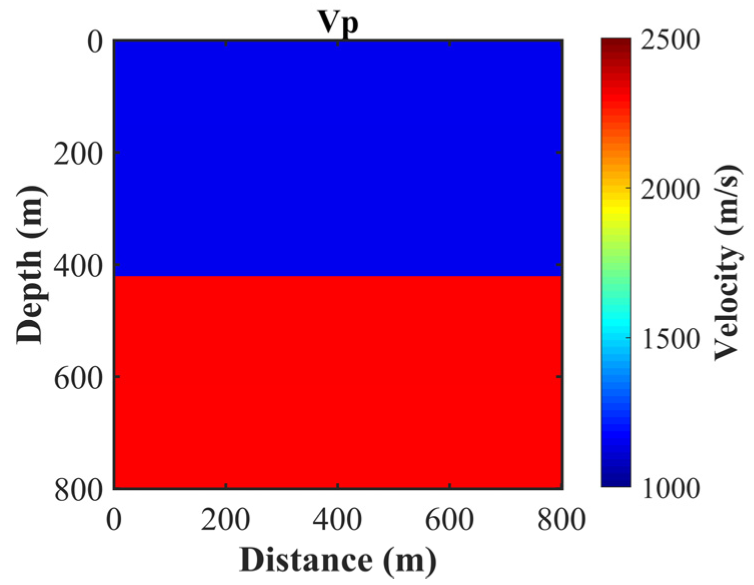
For a more comprehensive comparison of different collision operators, we examined a heterogeneous medium comprising two layers of homogeneous media connected at a horizontal interface with discrete grids of 801 × 801, as depicted in Figure 8. The lower layer exhibits a larger velocity in comparison to the upper layer. Both layers are assumed to possess a constant density value of 1000 kg/m³, and uniform spatial and temporal intervals are employed in the wave propagation simulations. The upper and lower layers’ velocities are 1155 m/s and 2310 m/s, while the source and receiving points are located at coordinates (401 m, 341 m) and (361 m, 361 m), respectively. The Ricker wavelet source has a dominant frequency of 50 Hz, and the relaxation time of the LBM-SRT model is 0.54. The guideline for choosing relaxation times in LBM-TRT and LBM-MRT is explained in Section 2.3. Notably, a shared relaxation time of 0.54, associated with the media’s viscosity, was used for all the models.
To validate and compare the wave simulation results from different LBM models, we have employed consistent parameters. The reference non-viscous wavefields were obtained by solving the acoustic equation using the classical FDM scheme.
Figure 9 shows the snapshots of Vz calculated with FDM-Acoustic and three LBM schemes by adopting the D2Q9 models. Due to the LBM’s relaxation time being close to 0.54, the viscosity effect on the simulated wavefield is minimal. As a result, the calculated waveforms of the three LBM models closely resemble that of FDM reference solution. The seismic records and corresponding amplitude spectra in Figure 10a,b demonstrate that the direct waves closely align with that of FDM, with slight variations in the amplitude values of the interface-reflected waves. This divergence is due to the computation of weakly viscous sound waves by LBM. Moreover, Figure 10b shows that there is relatively high consistency in the energy of the amplitude spectra of the wavefields, particularly in the middle and low-frequency bands, when comparing the spectra from the three LBM models with that of the FDM-calculated sound wave. However, in the high frequency range, the LBM-calculated wavefield energy is slightly weaker, owing to some attenuation. In order to further investigate the performance of different relaxation times under short relaxation time, Figure 10c,d also compare the simulation results when the relaxation time is 0.51. It is evident that when the relaxation time is closer to 0.50, the seismogram and its amplitude spectra from the LBM simulations closely resemble the results obtained with FDM, consistent with real-world observations. Simultaneously, we observe that when the relaxation time is set to 0.51, seismic records simulated by LBM-SRT exhibit distortion, resulting in a deviation from the FDM reference solution. In contrast, LBM-TRT and LBM-MRT still produce reasonable wavefields, highlighting the advantages of LBM-TRT and LBM-MRT over LBM-SRT.
4.2.2. Modified Marmousi Model
To further assess discrepancies between various LBM models when simulating seismic wave propagation within complex geological models, we devised the modified Marmousi model, depicted in Figure 11. The grid utilized for calculations is 801 × 801, with source point coordinates situated at (761 m, 601 m). The seismic source operates at a dominant frequency of 40 Hz, the LBM-SRT model employs a relaxation time of 0.80, and the settings of relaxation times for the LBM-TRT and LBM-MRT models are similar to that in Section 4.2.1. Similarly, FDM is employed to compute acoustic wavefields in the same model, serving as a reference solution.
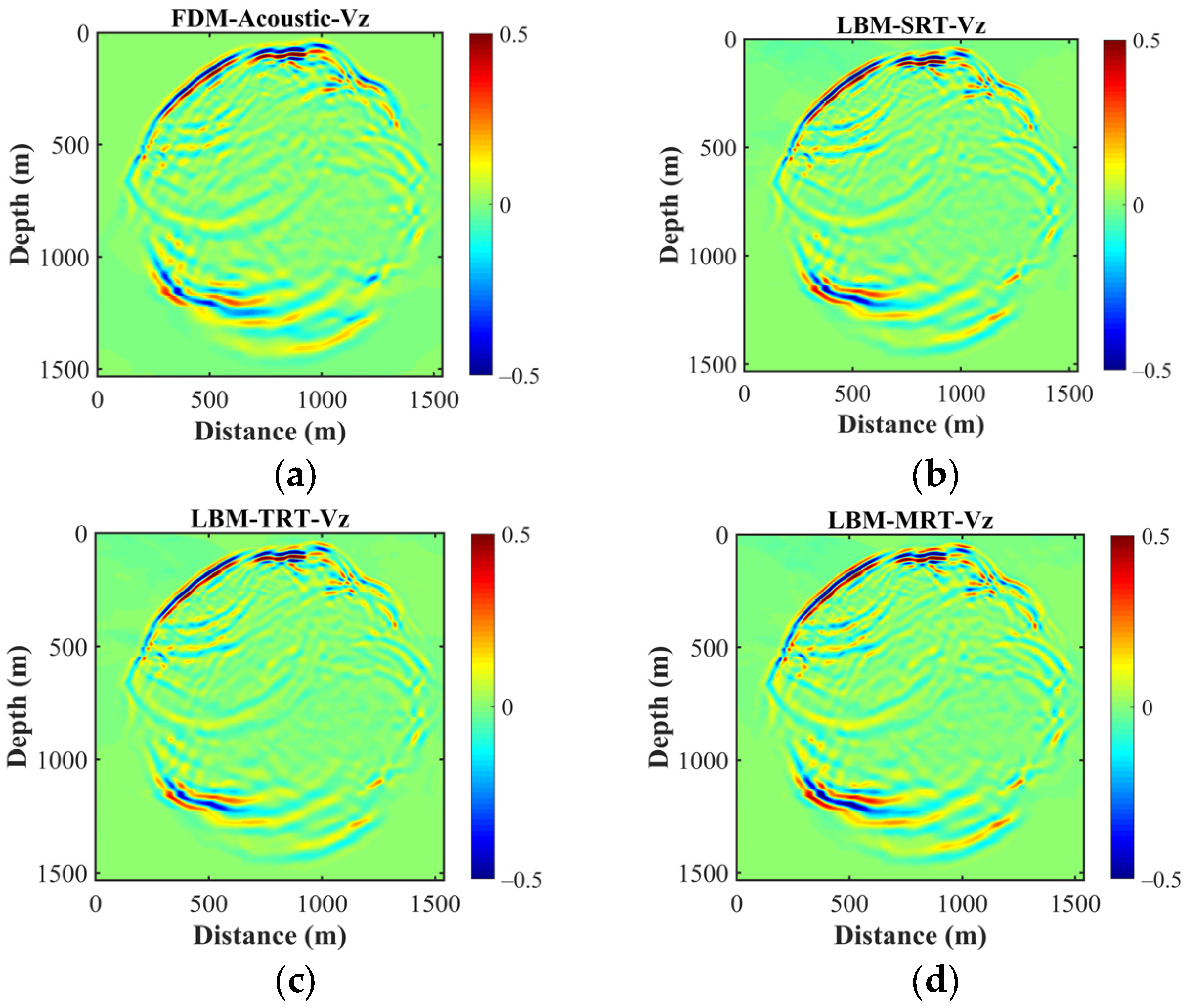
Figure 12 shows snapshots of Vz calculated using FDM and the three LBM models. The figures highlight that the general shape of the wavefield snapshots across the four methods is nearly identical, validating the coherence of wavefields calculated by the three LBM models. Nevertheless, nuances between the three LBM-calculated wavefields and the FDM reference solutions are observable in finer details, such as the direct wave in the lower right corner. Ultimately, through comparisons, we deduce that the wavefields computed using the three LBM models exhibit greater similarity among themselves than with FDM-calculated results. This underscores that while slight energy disparities may exist in seismic wave forward simulation outcomes using different LBM models, overall wavefield characteristics remain unaffected.
The assessment of different collision operators through the two-layer and modified Marmousi models demonstrates the robustness and reliability of LBM in simulating seismic wave propagation across varying geological scenarios. Despite nuanced energy variations, the essential wave propagation characteristics were preserved. The findings suggest that despite minor variations, wave snapshots, seismic records, and amplitude spectra generated by the different LBM models exhibit remarkable similarities. These results imply that the choice of the most suitable LBM model for practical seismic wave numerical simulations can be based on the simulated medium’s viscosity characteristics. For a low-viscosity medium, MRT provides better simulation results. In a medium with relatively high viscosity, the simulation outcomes of the three collision models are comparable. However, for cases requiring more refined characterization of medium viscosity, MRT demonstrates greater flexibility and stability compared with SRT and TRT.
Consequently, in practical seismic wave numerical simulations, the selection of the most suitable LBM model can be based on the simulated medium’s kinematic and dynamic viscosity characteristics. These insights offer practitioners valuable guidance in selecting suitable LBM collision operators for seismic simulations in various geological settings.
5. Discussion
We have undertaken a comprehensive investigation to compare and analyze wavefields generated through the utilization of different relaxation times, discrete velocity models, and collision operators within the framework of the LBM. The purpose of our analysis was to gain insights into how these parameters influence the characteristics of wave propagation and to discern the optimal combinations for accurately representing wave phenomena.
Our examination of five relaxation time values of 0.50, 0.51, 0.65, 0.80, and 1.00 revealed distinct impacts on the generated wavefields. A smaller relaxation time accelerates the relaxation process and results in quicker equilibration of distribution functions and, consequently, reduced energy consumption. Conversely, larger relaxation times dampen the wave propagation and lead to more obvious phase distortion. The choice of relaxation time should therefore be guided by the desired wave attenuation characteristics and the physical accuracy required for the simulation.
The wavefields calculated using the four discrete velocity models, namely, D2Q4, D2Q5, D2Q9, and D2Q13, showcased diverse behaviors in wave propagation. Models with a larger number of discrete velocities, such as D2Q13, generally exhibited improved representation of waveforms due to their finer spatial resolution. However, the computational cost associated with these models also increased. For scenarios where computational efficiency is crucial, a trade-off between accuracy and computational load needs to be considered when selecting a discrete velocity model.
Our investigation also encompassed three collision operators, i.e., SRT, TRT, and MRT. The choice of collision operator plays a pivotal role in controlling the relaxation process and thereby influencing wave propagation behavior. The SRT operator introduces a single relaxation time, resulting in a uniform relaxation process across all velocity directions. While computationally efficient, it may not accurately capture complex wave interactions, especially in scenarios with varying relaxation factors. The TRT operator’s ability to incorporate distinct relaxation times for different distribution function modes enhances its capability to represent non-equilibrium wave phenomena. This makes it a valuable choice for simulations requiring accurate wavefield representation. The MRT operator’s multiple relaxation parameters and transformation matrices provide a more nuanced control over relaxation dynamics. It excels in simulating wavefields with anisotropic and turbulent characteristics, although at the expense of increased computational complexity.
The findings of our study emphasize the interconnectedness of relaxation times, discrete velocity models, and collision operators in shaping wavefields within the LBM framework. Researchers and practitioners should consider these interdependencies while selecting appropriate parameter combinations for specific simulation scenarios.
6. Conclusions
In this study, we embarked on a comprehensive exploration of wavefield simulations within the LBM, focusing on the interplay between relaxation times, discrete velocity models, and collision operators. Through a systematic investigation, we have gained valuable insights on the behavior of wavefields simulated using LBM, as follows:
- (1)
- Relaxation time. We observed that the choice of relaxation time profoundly influences wave propagation speed. Small relaxation times (i.e., around 0.50) yield more fidelity seismic recording and higher wavefield energy, while larger relaxation times dampen wave propagation. The choice of a suitable relaxation time depends on the desired wave dynamics and the level of physical fidelity required in the simulation.
- (2)
- Discrete velocity models. Our analysis revealed that discrete velocity models with a larger number of velocities provide finer spatial resolution and more accurate wavefield representation. However, this comes at the cost of increased computational complexity. The trade-off between accuracy and computational efficiency must be carefully considered when choosing a discrete velocity model.
- (3)
- Collision operators. The collision operator plays a crucial role in dictating relaxation dynamics and consequently influences the wave propagation behavior. While the SRT model offers computational efficiency, it may not capture complex wave interactions accurately. The TRT and MRT models, with their ability to accommodate different relaxation factors, excel in representing non-equilibrium wave phenomena and anisotropic behaviors.
These insights can guide the development of hybrid approaches that combine the strengths of different relaxation times, discrete velocity models, and collision operators to achieve higher accuracy and efficiency in wavefield simulations. Future research avenues could include in-depth analyses of the interactions between these parameters in more specialized scenarios, such as multiphase flows, turbulent environments, and complex geometries. Additionally, extending this comparative analysis to other types of waves, such as aero-acoustic, electromagnetic, or elastic waves, could broaden the applicability of our findings to an even wider range of physical phenomena.
Author Contributions
Conceptualization, M.X. and H.Z.; formal analysis, M.X. and C.J.; methodology, M.X. and C.J.; software, M.X. and C.J.; supervision, H.Z. and H.C.; writing—original draft, M.X., C.J. and J.C.; writing—review and editing, H.Z. and Y.Z. All authors have read and agreed to the published version of the manuscript.
Funding
This work was supported in part by the R&D Department of CNPC (2022DQ0604-01), National Natural Science Foundation of China (42204132), and the China Postdoctoral Science Foundations (2020M680667, 2021T140661). M.X. greatly acknowledges the financial support from the CAS Special Research Assistant Project.
Data Availability Statement
The data used in this study are available by contacting the corresponding author. The data are not publicly available due to privacy.
Conflicts of Interest
The authors declare no conflict of interest.
References
- Tarantola, A. Inversion of seismic reflection data in the acoustic approximation. Geophysics 1984, 49, 1259–1266. [Google Scholar] [CrossRef]
- Tarantola, A. A strategy for nonlinear elastic inversion of seismic reflection data. Geophysics 1986, 51, 1893–1903. [Google Scholar] [CrossRef]
- Virieux, J.; Operto, S. An overview of full-waveform inversion in exploration. Geophysics 2009, 74, WCC1–WCC26. [Google Scholar] [CrossRef]
- Aghamiry, H.S.; Gholami, A.; Operto, S. Compound regularization of full-waveform inversion for imaging piecewise media. IEEE Trans. Geosci. Remote Sens. 2020, 58, 1192–1204. [Google Scholar] [CrossRef]
- Zhang, Q.C.; Mao, W.J.; Fang, J.W. Elastic full waveform inversion with source-independent crosstalk-free source-encoding algorithm. IEEE Trans. Geosci. Remote Sens. 2020, 58, 2915–2927. [Google Scholar] [CrossRef]
- Hu, Y.; Fu, L.Y.; Li, Q.Q.; Deng, W.B.; Han, L.G. Frequency-wavenumber domain elastic full waveform inversion with a multistage phase correction. Remote Sens. 2022, 14, 5916. [Google Scholar] [CrossRef]
- Feng, D.S.; Li, B.C.; Cao, C.; Wang, X.; Li, D.B.; Chen, C. Multi-constrained seismic multi-parameter full waveform inversion based on projected quasi-Newton algorithm. Remote Sens. 2023, 15, 2416. [Google Scholar] [CrossRef]
- Baysal, E.; Kosloff, D.D.; Sherwood, J.W.C. Reverse time migration. Geophysics 1983, 48, 1514–1524. [Google Scholar] [CrossRef]
- Chattopadhyay, S.; McMechan, G.A. Imaging conditions for prestack reverse-time migration. Geophysics 2008, 73, S81–S89. [Google Scholar] [CrossRef]
- Li, Q.Q.; Fu, L.Y.; Wei, W.; Sun, W.J.; Du, Q.Z.; Feng, Y.S. Stable and high-efficiency attenuation compensation in reverse-time migration using wavefield decomposition algorithm. IEEE Geosci. Remote Sens. 2019, 16, 1615–1619. [Google Scholar] [CrossRef]
- Li, Q.Q.; Fu, L.Y.; Wu, R.S.; Du, Q.Z. A novel wavefield-reconstruction algorithm for RTM in attenuating media. IEEE Geosci. Remote Sens. 2021, 18, 731–735. [Google Scholar] [CrossRef]
- Shen, R.Q.; Zhao, Y.H.; Hu, S.F.; Li, B.; Bi, W.D. Reverse-time migration imaging of ground-penetrating radar in NDT of reinforced concrete structures. Remote Sens. 2021, 13, 2020. [Google Scholar] [CrossRef]
- Wang, N.; Shi, Y.; Zhou, H. Accurately stable Q-compensated reverse-time migration scheme for heterogeneous viscoelastic media. Remote Sens. 2022, 14, 4782. [Google Scholar] [CrossRef]
- Fang, J.W.; Shi, Y.; Zhou, H. A high-precision elastic reverse-time migration for complex geologic structure imaging in applied geophysics. Remote Sens. 2022, 14, 3542. [Google Scholar] [CrossRef]
- Chen, S.Y.; Chen, H.D.; Martnez, D.; Matthaeus, W. Lattice Boltzmann model for simulation of magnetohydrodynamics. Phys. Rev. Lett. 1991, 67, 3776–3779. [Google Scholar] [CrossRef] [PubMed]
- Koelman, J.M.V.A. A simple lattice Boltzmann scheme for Navier-Stokes fluid flow. Europhys. Lett. 1991, 15, 603–607. [Google Scholar] [CrossRef]
- Qian, Y.H.; d’Humières, D.; Lallemand, P. Lattice BGK models for Navier-Stokes equation. Europhys. Lett. 1992, 17, 479–484. [Google Scholar] [CrossRef]
- Xiao, S. A lattice Boltzmann method for shock wave propagation in solids. Commun. Numer. Methods Eng. 2007, 23, 71–84. [Google Scholar] [CrossRef]
- Zhang, J.Y.; Yan, G.W.; Shi, X.B. Lattice Boltzmann model for wave propagation. Phys. Rev. E 2009, 80, 026706. [Google Scholar] [CrossRef]
- Frantziskonis, G.N. Lattice Boltzmann method for multimode wave propagation in viscoelastic media and in elastic solids. Phys. Rev. E 2011, 283, 066703. [Google Scholar] [CrossRef]
- Viggen, E.M. The Lattice Boltzmann Method with Applications in Acoustics. Master’s Thesis, Norwegian University of Science and Technology, Trondheim, Norway, 2009; pp. 1–95. [Google Scholar]
- Viggen, E.M. The Lattice Boltzmann Method: Fundamentals and Acoustics. Ph.D. Thesis, Norwegian University of Science and Technology, Trondheim, Norway, 2014; pp. 1–233. [Google Scholar]
- Salomons, E.M.; Lohman, W.J.A.; Zhou, H. Simulation of sound waves using the lattice Boltzmann method for fluid flow: Benchmark cases for outdoor sound propagation. PLoS ONE 2016, 11, e0147206. [Google Scholar] [CrossRef]
- Jiang, C.T.; Zhou, H.; Xia, M.M.; Tang, J.X.; Zhang, M.K.; An, Y. Study on absorbing boundary conditions of viscous sponge layers based on lattice Boltzmann method. In Proceedings of the 82nd EAGE Annual Conference & Exhibition, Amsterdam, The Netherlands, 8–11 December 2020; pp. 1–5. [Google Scholar]
- Xia, M.M.; Wang, S.C.; Zhou, H.; Shan, X.W.; Chen, H.M.; Li, Q.Q.; Zhang, Q.C. Modelling viscoacoustic wave propagation with the lattice Boltzmann method. Sci. Rep. 2017, 7, 10169. [Google Scholar] [CrossRef] [PubMed]
- Xia, M.M.; Zhou, H.; Jiang, C.T.; Tang, J.X.; Wang, C.Y.; Yang, C.C. Viscoacoustic wave simulation with the lattice Boltzmann method. Geophysics 2022, 87, T403–T416. [Google Scholar] [CrossRef]
- Ginzburg, I. Equilibrium-type and link-type lattice Boltzmann models for generic advection and anisotropic-dispersion equation. Adv. Water Resour. 2005, 28, 1171–1195. [Google Scholar] [CrossRef]
- Servan-Camas, B.; Tsai, F.T.C. Lattice Boltzmann method with two relaxation times for advection–diffusion equation: Third order analysis and stability analysis. Adv. Water Resour. 2008, 31, 1113–1126. [Google Scholar] [CrossRef]
- Talon, L.; Bauer, D.; Gland, N.; Youssef, S.; Auradou, H.; Ginzburg, I. Assessment of the two relaxation time Lattice-Boltzmann scheme to simulate Stokes flow in porous media. Water Resour. Res. 2012, 48, W04526. [Google Scholar] [CrossRef]
- Vikhansky, A.; Ginzburg, I. Taylor dispersion in heterogeneous porous media: Extended method of moments, theory, and modelling with two-relaxation-times lattice Boltzmann scheme. Phys. Fluids 2014, 26, 22104. [Google Scholar] [CrossRef]
- Peng, Y.; Zhang, J.M.; Zhou, J.G. Lattice Boltzmann model using two relaxation times for shallow-water equations. J. Hydraul. Eng. 2016, 142, 06015017. [Google Scholar] [CrossRef]
- Zhao, W.F.; Wang, L.; Yong, W.A. On a two-relaxation-time D2Q9 lattice Boltzmann model for the Navier–Stokes equations. Physica A Stat. Mech. Appl. 2018, 492, 1570–1580. [Google Scholar] [CrossRef]
- Bhopalam, S.R.; Perumal, D.A.; Yadav, A.K. Computation of fluid flow in double sided cross-shaped lid-driven cavities using lattice Boltzmann method. Eur. J. Mech. B-Fluid 2018, 70, 46–72. [Google Scholar]
- Postma, B.; Silva, G. Force methods for the two-relaxation-times lattice Boltzmann. Phys. Rev. E 2020, 102, 063307. [Google Scholar] [CrossRef] [PubMed]
- D’Humières, D. Generalized lattice-Boltzmann equations, in Rarefied Gas Dynamics: Theory and Simulations. In Progress in Astronautics and Aeronautics; Shizgal, B.D., Weave, D.P., Eds.; AIAA: Washington, DC, USA, 1992; Volume 159, pp. 450–458. [Google Scholar]
- D’Humières, D. Multiple-relaxation-time lattice Boltzmann models in three dimensions. Philos. Trans. R. Soc. Lond. Ser. A 2002, 360, 437–451. [Google Scholar] [CrossRef] [PubMed]
- Fakhari, A.; Rahimian, M.H. Phase-field modeling by the method of lattice Boltzmann equations. Phys. Rev. E 2010, 81, 036707. [Google Scholar] [CrossRef]
- Zhao, Z.M.; Huang, P.; Li, Y.N.; Li, J.M. A lattice Boltzmann method for viscous free surface waves in two dimensions. Int. J. Numer. Methods Fluids 2013, 71, 223–248. [Google Scholar] [CrossRef]
- Wang, J.; Wang, D.; Lallemand, P.; Luo, L.S. Lattice Boltzmann simulations of thermal convective flows in two dimensions. Comput. Math. Appl. 2013, 65, 262–286. [Google Scholar] [CrossRef]
- Dhuri, D.B.; Hanasoge, S.M.; Perlekar, P.; Robertsson, J.O. Numerical analysis of the lattice Boltzmann method for simulation of linear acoustic waves. Phys. Rev. E 2017, 95, 043306. [Google Scholar] [CrossRef] [PubMed]
- Chai, Z.H.; Shi, B.C. Multiple-relaxation-time lattice Boltzmann method for the Navier-Stokes and nonlinear convection-diffusion equations: Modeling, analysis, and elements. Phys. Rev. E 2020, 102, 023306. [Google Scholar] [CrossRef]
- Benhamou, J.; Jami, M.; Mezrhab, A.; Henry, D.; Botton, V. Numerical simulation study of acoustic waves propagation and streaming using MRT-lattice Boltzmann method. Int. J. Comput. Methods Eng. Sci. Mech. 2023, 24, 62–75. [Google Scholar] [CrossRef]
- Jiang, C.T.; Zhou, H.; Xia, M.M.; Chen, H.M.; Tang, J.X. A joint absorbing boundary for the multiple-relaxation-time lattice Boltzmann method in seismic acoustic wavefield modeling. Pet. Sci. 2023, 20, 2113–2126. [Google Scholar] [CrossRef]
- Qian, Y.H.; Deng, Y.F. A lattice BGK model for viscoelastic media. Phys. Rev. 1997, 79, 2742–2745. [Google Scholar] [CrossRef]
- Buick, J.M.; Buckley, C.L.; Greated, C.A. Lattice Boltzmann BGK simulation of nonlinear sound waves: The development of a shock front. J. Phys. A Math. Gen. 2000, 33, 3917. [Google Scholar] [CrossRef]
- Xia, Y.X.; Qiu, X.; Qian, Y.H. Numerical simulation of two-dimensional turbulence based on immersed boundary lattice Boltzmann method. Comput. Fluids 2019, 195, 104321. [Google Scholar] [CrossRef]
- Ezzatneshan, E.; Salehi, A.; Vaseghnia, H. Study on forcing schemes in the thermal lattice Boltzmann method for simulation of natural convection flow problems. Heat Transfer 2021, 50, 7604–7631. [Google Scholar] [CrossRef]
- Luo, L.S.; Liao, W.; Chen, X.W.; Peng, Y.; Zhang, W. Numerics of the lattice Boltzmann method: Effects of collision models on the lattice Boltzmann simulations. Phys. Rev. E 2011, 83, 056710. [Google Scholar] [CrossRef]
- Lallemand, P.; Luo, L.S. Theory of the lattice Boltzmann method: Dispersion, dissipation, isotropy, Galilean invariance, and stability. Phys. Rev. E 2000, 61, 6546–6562. [Google Scholar] [CrossRef]
- Aslan, E.; Taymaz, I.; Benim, A.C. Investigation of the lattice Boltzmann SRT and MRT stability for lid driven cavity flow. Int. J. Mater. Mech. Manuf. 2014, 2, 317–324. [Google Scholar]
- Haydock, D.; Yeomans, J.M. Lattice Boltzmann simulations of attenuation-driven acoustic streaming. J. Phys. A Math. Gen. 2003, 36, 5683–5694. [Google Scholar] [CrossRef]
Figure 1.
Sketch maps of the discrete velocity sets for the 2D LBM models. (a) D2Q4, (b) D2Q5, (c) D2Q9, and (d) D2Q13.
Figure 1.
Sketch maps of the discrete velocity sets for the 2D LBM models. (a) D2Q4, (b) D2Q5, (c) D2Q9, and (d) D2Q13.

Figure 2.
Comparison of the normalized phase velocity curves of the four LBM models for different angles of (a) 0°, (b) 15°, (c) 30°, and (d) 45°. Nλ represents the number of discrete points per wavelength.
Figure 2.
Comparison of the normalized phase velocity curves of the four LBM models for different angles of (a) 0°, (b) 15°, (c) 30°, and (d) 45°. Nλ represents the number of discrete points per wavelength.
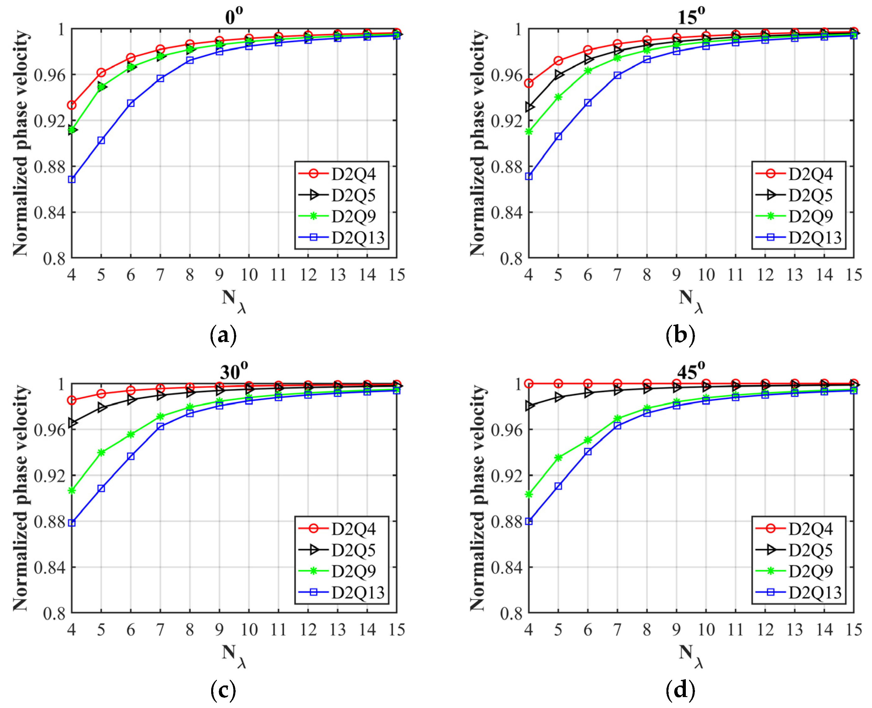
Figure 3.
Comparison of the spatial variation of the relative errors of the normalized phase velocities for the four different LBM discrete models of (a) D2Q4, (b) D2Q5, (c) D2Q9, and (d) D2Q13.
Figure 3.
Comparison of the spatial variation of the relative errors of the normalized phase velocities for the four different LBM discrete models of (a) D2Q4, (b) D2Q5, (c) D2Q9, and (d) D2Q13.
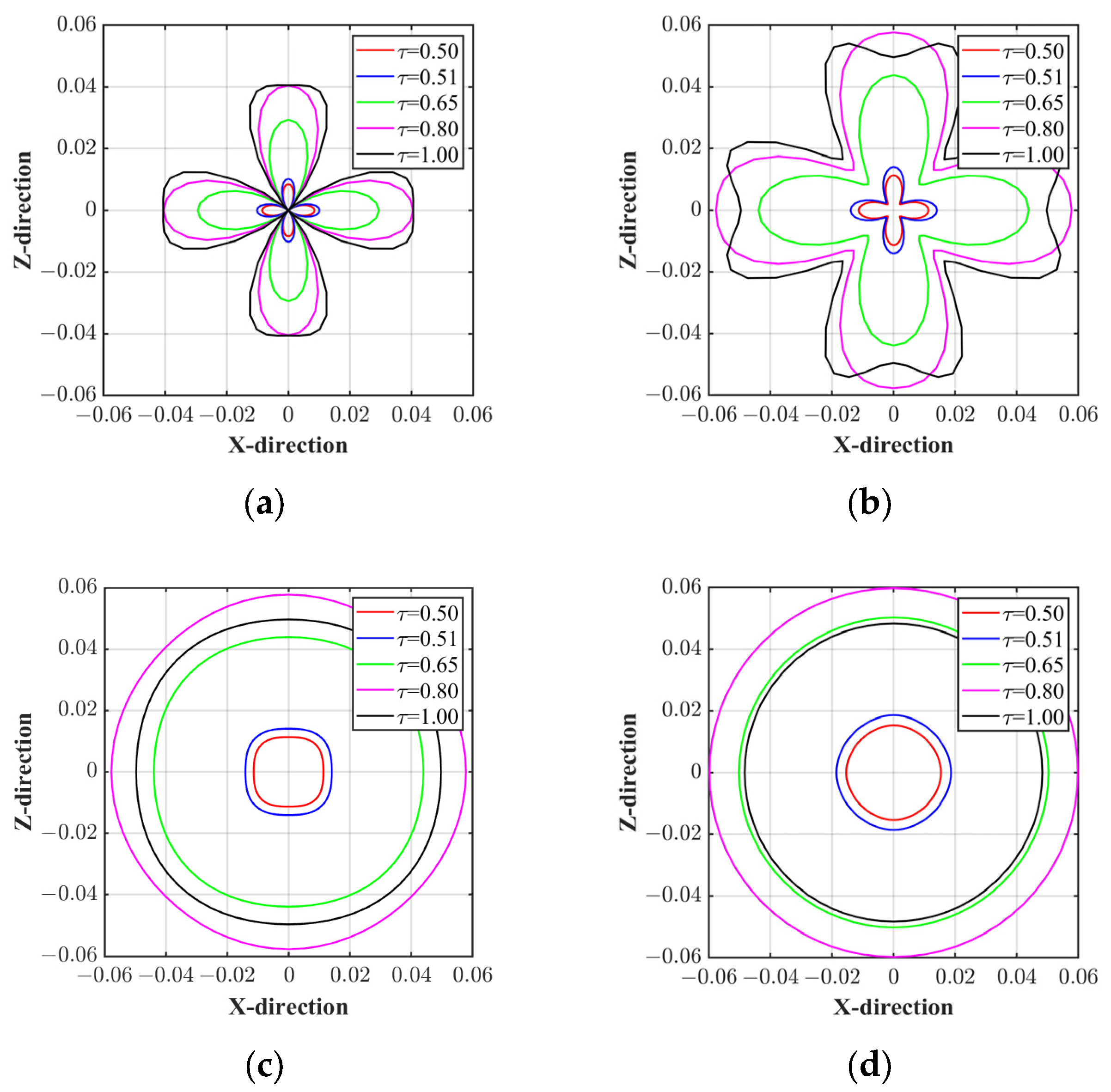
Figure 4.
Comparison of the seismic snapshots of LBM with four discrete velocity models of (a) D2Q4, (b) D2Q5, (c) D2Q9, and (d) D2Q13, and four different relaxation times of 0.51, 0.65, 0.80, and 1.00 in homogeneous medium.
Figure 4.
Comparison of the seismic snapshots of LBM with four discrete velocity models of (a) D2Q4, (b) D2Q5, (c) D2Q9, and (d) D2Q13, and four different relaxation times of 0.51, 0.65, 0.80, and 1.00 in homogeneous medium.
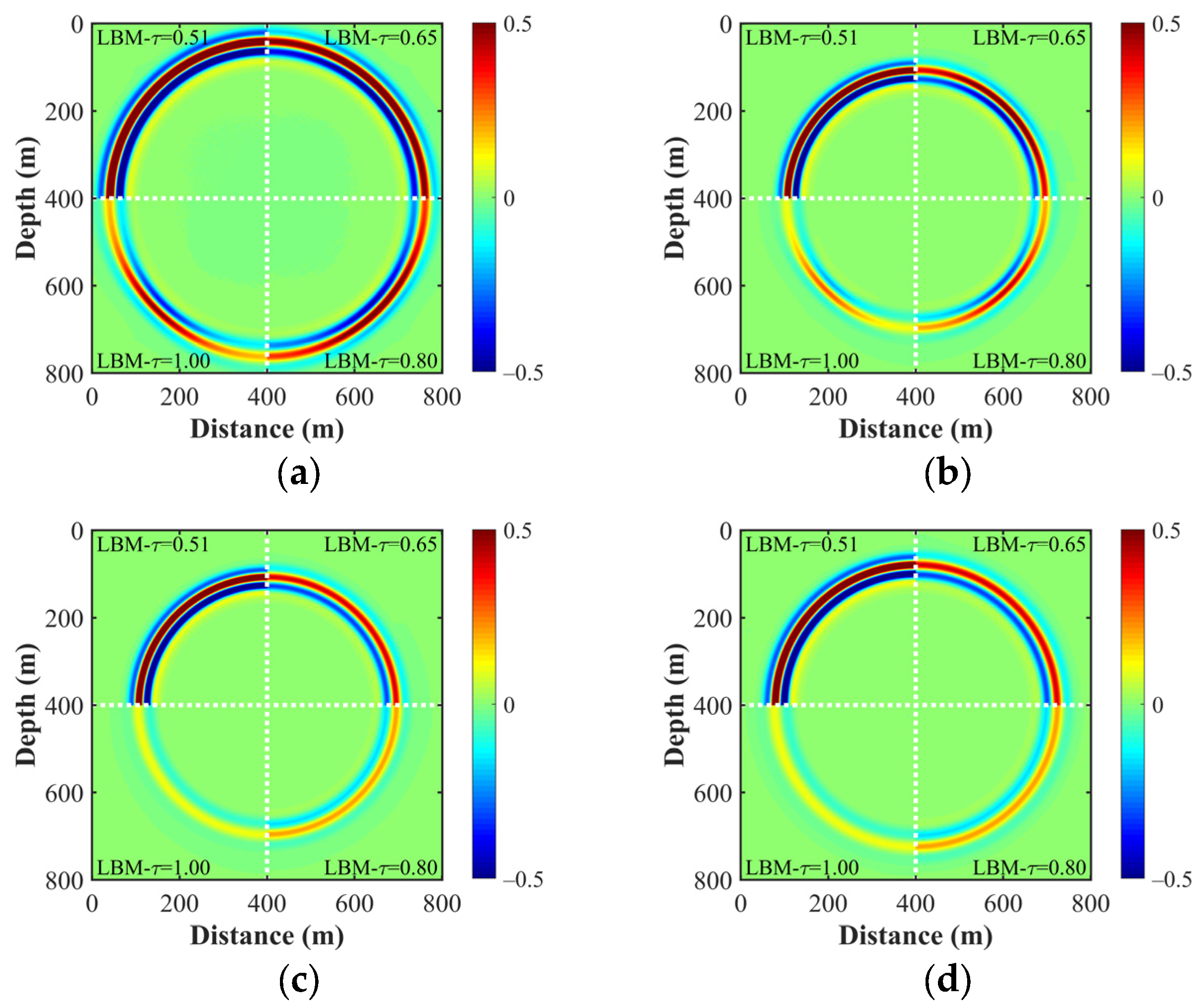
Figure 5.
Comparison of the seismic traces computed using LBM with four discrete velocity models of (a) D2Q4, (b) D2Q5, (c) D2Q9, and (d) D2Q13, and five different relaxation times of 0.50, 0.51, 0.65, 0.80, and 1.00 in the homogeneous medium.
Figure 5.
Comparison of the seismic traces computed using LBM with four discrete velocity models of (a) D2Q4, (b) D2Q5, (c) D2Q9, and (d) D2Q13, and five different relaxation times of 0.50, 0.51, 0.65, 0.80, and 1.00 in the homogeneous medium.

Figure 6.
Comparison of the spectra of seismic traces calculated using LBM with four discrete velocity models of (a) D2Q4, (b) D2Q5, (c) D2Q9, and (d) D2Q13, and five different relaxation times of 0.50, 0.51, 0.65, 0.80, and 1.00 in a homogeneous medium.
Figure 6.
Comparison of the spectra of seismic traces calculated using LBM with four discrete velocity models of (a) D2Q4, (b) D2Q5, (c) D2Q9, and (d) D2Q13, and five different relaxation times of 0.50, 0.51, 0.65, 0.80, and 1.00 in a homogeneous medium.
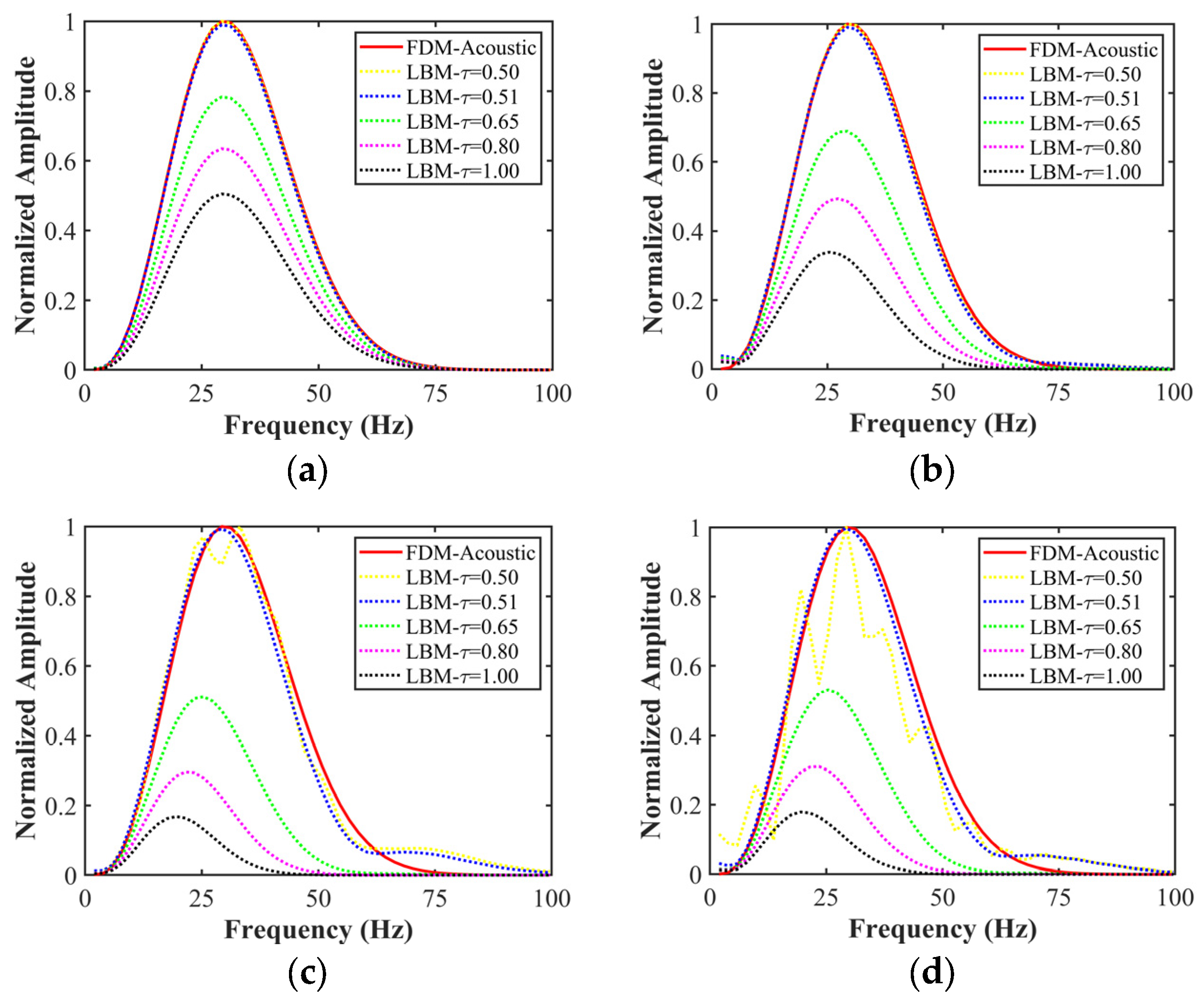
Figure 7.
(a) Snapshots, (b) seismic traces, and the corresponding (c) amplitude spectra obtained with FDM-Acoustic and LBM with four different discrete velocity models of D2Q4, D2Q5, D2Q9, and D2Q13 with .
Figure 7.
(a) Snapshots, (b) seismic traces, and the corresponding (c) amplitude spectra obtained with FDM-Acoustic and LBM with four different discrete velocity models of D2Q4, D2Q5, D2Q9, and D2Q13 with .
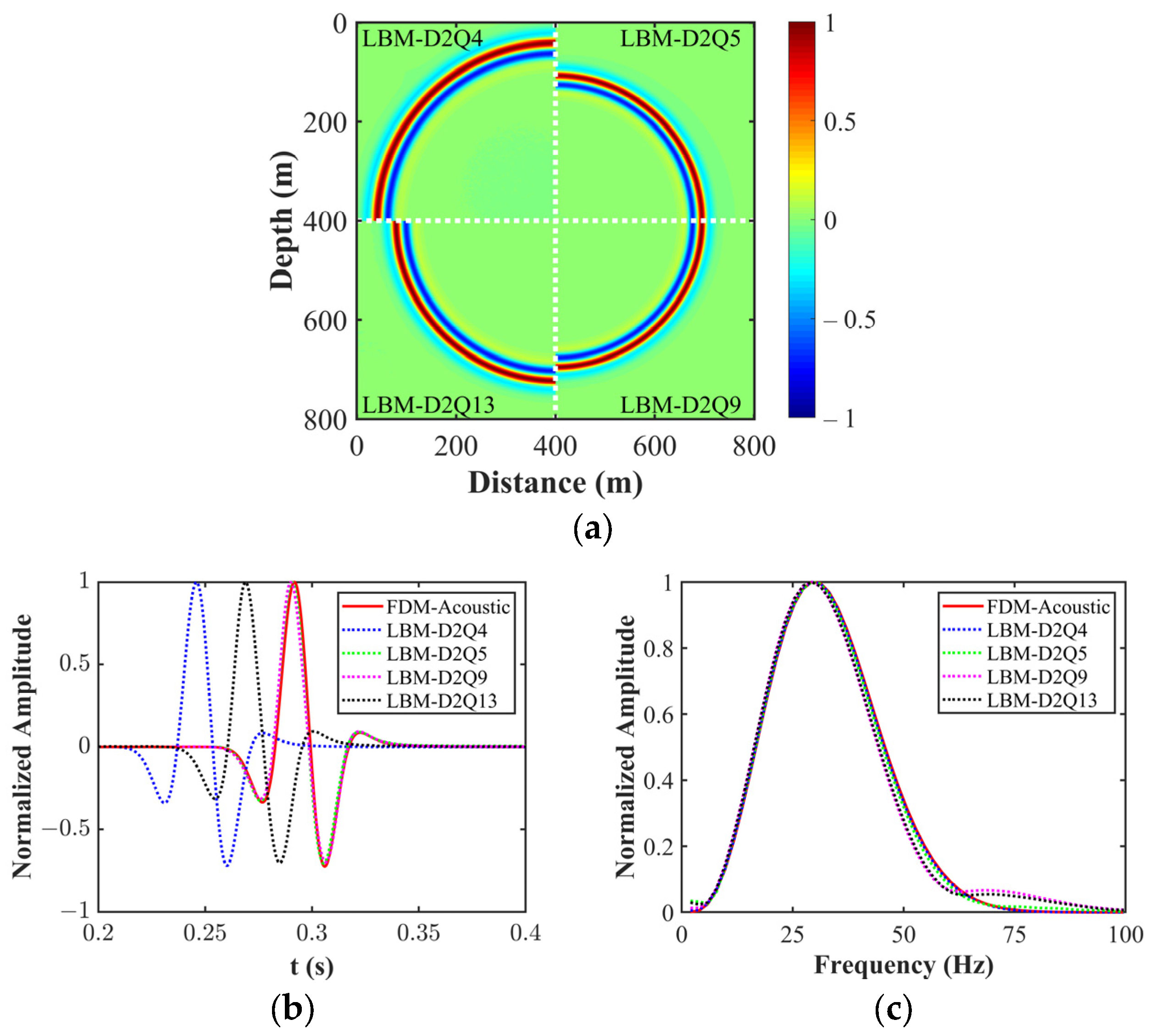
Figure 8.
Two-layer model.

Figure 9.
Snapshots of Vz calculated with (a) FDM-Acoustic, (b) LBM-SRT, (c) LBM-TRT, and (d) LBM-MRT in the two-layer model.
Figure 9.
Snapshots of Vz calculated with (a) FDM-Acoustic, (b) LBM-SRT, (c) LBM-TRT, and (d) LBM-MRT in the two-layer model.

Figure 10.
(a) Seismic records and the corresponding (b) amplitude spectra of Vz calculated with FDM-Acoustic and the three LBM models in the two-layer model with a relaxation time of 0.54; (c) seismic records and the corresponding (d) amplitude spectra of Vz calculated with FDM-Acoustic and the three LBM models in the two-layer model with a relaxation time of 0.51.
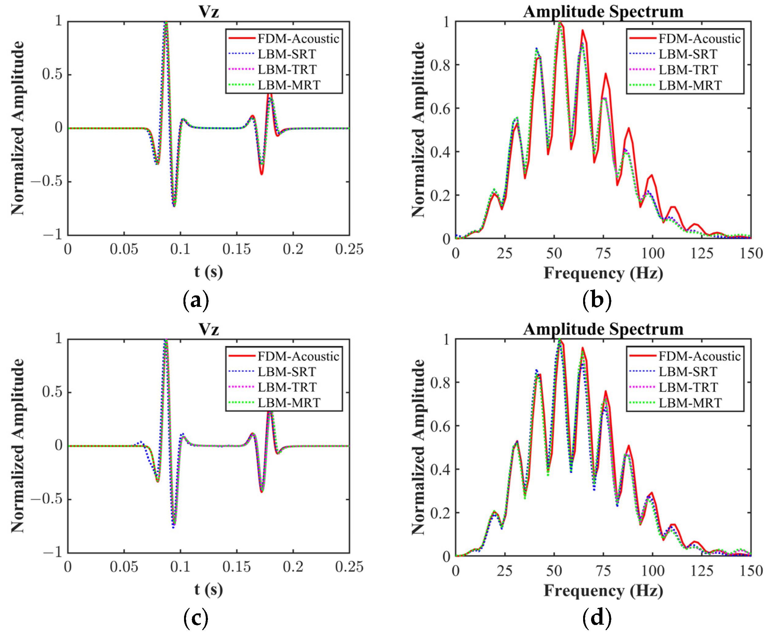
Figure 11.
Vp of the modified Marmousi model.
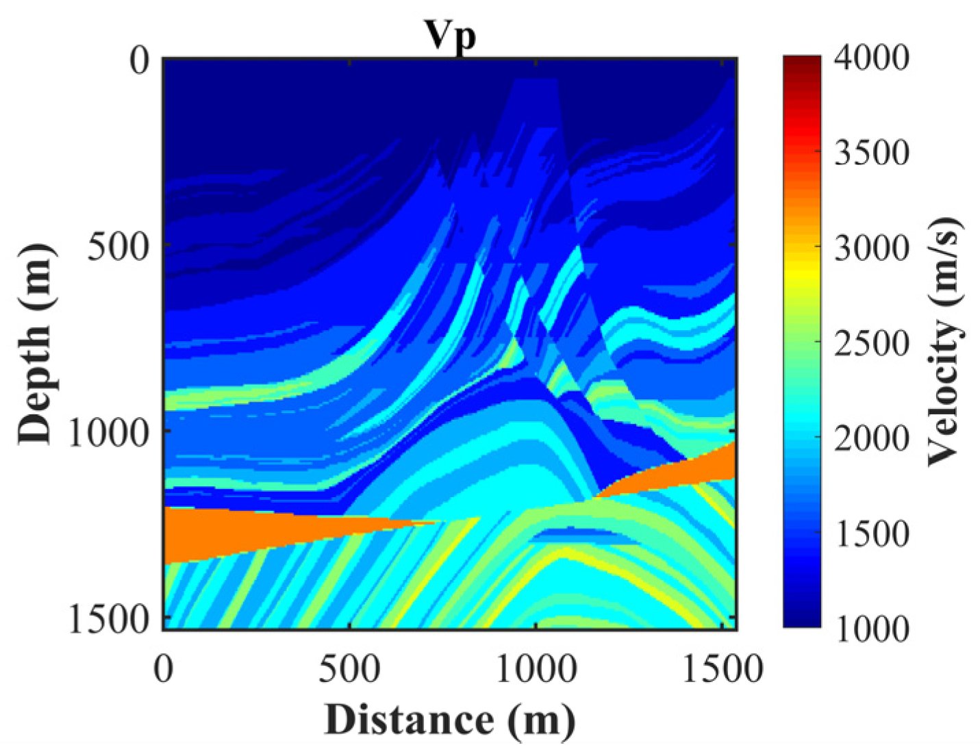
Figure 12.
Snapshots of Vz in the modified Marmousi model calculated with (a) FDM, (b) LBM-SRT, (c) LBM-TRT, and (d) LBM-MRT.
Figure 12.
Snapshots of Vz in the modified Marmousi model calculated with (a) FDM, (b) LBM-SRT, (c) LBM-TRT, and (d) LBM-MRT.


Table 1.
Comparison of the discrete velocity sets, weights, and lattice sound speeds for the 2D LBM discrete models.
Table 1.
Comparison of the discrete velocity sets, weights, and lattice sound speeds for the 2D LBM discrete models.
| Discrete Models | |||
|---|---|---|---|
| D2Q4 | 1/2 | ||
| D2Q5 | 1/3 | ||
| D2Q9 | 1/3 | ||
| D2Q13 | 2/5 |
Disclaimer/Publisher’s Note: The statements, opinions and data contained in all publications are solely those of the individual author(s) and contributor(s) and not of MDPI and/or the editor(s). MDPI and/or the editor(s) disclaim responsibility for any injury to people or property resulting from any ideas, methods, instructions or products referred to in the content. |
© 2024 by the authors. Licensee MDPI, Basel, Switzerland. This article is an open access article distributed under the terms and conditions of the Creative Commons Attribution (CC BY) license (https://creativecommons.org/licenses/by/4.0/).
Share and Cite
MDPI and ACS Style
Xia, M.; Zhou, H.; Jiang, C.; Cui, J.; Zeng, Y.; Chen, H. Comparative Study of 2D Lattice Boltzmann Models for Simulating Seismic Waves. Remote Sens. 2024, 16, 285. https://doi.org/10.3390/rs16020285
AMA Style
Xia M, Zhou H, Jiang C, Cui J, Zeng Y, Chen H. Comparative Study of 2D Lattice Boltzmann Models for Simulating Seismic Waves. Remote Sensing. 2024; 16(2):285. https://doi.org/10.3390/rs16020285
Chicago/Turabian StyleXia, Muming, Hui Zhou, Chuntao Jiang, Jinming Cui, Yong Zeng, and Hanming Chen. 2024. "Comparative Study of 2D Lattice Boltzmann Models for Simulating Seismic Waves" Remote Sensing 16, no. 2: 285. https://doi.org/10.3390/rs16020285
Note that from the first issue of 2016, this journal uses article numbers instead of page numbers. See further details here.