Self-Attention Generative Adversarial Network Interpolating and Denoising Seismic Signals Simultaneously

Abstract

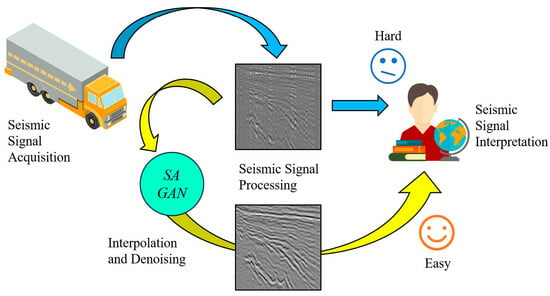
In light of the challenging conditions of exploration environments coupled with escalating exploration expenses, seismic data acquisition frequently entails the capturing of signals entangled amidst diverse noise interferences and instances of data loss. The unprocessed state of these seismic signals significantly jeopardizes the interpretative phase. Evidently, the integration of attention mechanisms and the utilization of generative adversarial networks (GANs) have emerged as prominent techniques within signal processing owing to their adeptness in discerning intricate global dependencies. Our research introduces a pioneering approach for reconstructing and denoising seismic signals, amalgamating the principles of self-attention and generative adversarial networks—hereafter referred to as SAGAN. Notably, the incorporation of the self-attention mechanism into the GAN framework facilitates an enhanced capacity for both the generator and discriminator to emulate meaningful spatial interactions. Subsequently, leveraging the feature map generated by the self-attention mechanism within the GAN structure enables the interpolation and denoising of seismic signals. Rigorous experimentation substantiates the efficacy of SAGAN in simultaneous signal interpolation and denoising. Initially, we benchmarked SAGAN against prominent methods such as UNet, CNN, and Wavelet for the concurrent interpolation and denoising of two-dimensional seismic signals manifesting varying levels of damage. Subsequently, this methodology was extended to encompass three-dimensional seismic data. Notably, performance metrics reveal SAGAN’s superiority over comparative methods. Specifically, the quantitative tables exhibit SAGAN’s pronounced advantage, with a 3.46% increase in PSNR value over UNet and an impressive 11.90% surge compared to Wavelet. Moreover, the RMSE values affirm SAGAN’s robust performance, showcasing an 11.54% reduction in comparison to UNet and an impressive 29.27% decrement relative to Wavelet, hence unequivocally establishing the SAGAN method as a preeminent choice for seismic signal recovery.

1. Introduction

Most advanced seismic signal processing methods, such as reverse time migration (RTM) [1], full waveform inversion (FWI) [2], and surface-related multiple elimination (SRME) [3], benefit from high-quality seismic signals. Based on high-quality seismic signals, we can also map geological structures and explore mineral resources. However, in field seismic exploration, the signal is often missing or contains noise due to the harsh acquisition environment and poor construction conditions. The presence of incomplete signals tainted by noise not only leads to the forfeiture of crucial information but also exerts detrimental effects on subsequent processing stages. Hence, the interpolation and denoising of seismic signals emerge as a pivotal endeavor in the realm of seismic exploration [4,5,6,7], holding profound significance in ensuring the fidelity and integrity of the data employed in this field.

Investigations into seismic signal interpolation and denoising methods can be broadly categorized into two primary methodologies: traditional approaches founded on model-driven principles and deep learning techniques rooted in data-driven paradigms.

Sparse transformation methods within traditional approaches have been extensively employed in the domain of seismic signal interpolation and denoising. For instance, Hindriks and Duijndam [8] introduced the concept of minimum norm Fourier reconstruction, employing Fourier transformation on non-uniformly sampled data to derive Fourier coefficients and subsequently utilizing inverse Fourier transformation to yield a uniform time domain signal. In a similar vein, Satish et al. [9] pioneered a novel methodology to compute the time–frequency map of non-stationary signals via continuous Wavelet transform. Additionally, Jones and Levy [10] harnessed the K-L transform to reconstruct seismic signals and suppress multiples within CMP or CDP datasets. These methodologies, grounded in sparse transformation, often employ iterative techniques and leverage sparse transformations. Predominantly, the transformations utilized presently rely on fixed basis functions. However, a persisting challenge lies in the selection of appropriate basis functions to achieve a sparser representation of the data. The optimization of basis function selection to yield enhanced sparsity remains an ongoing concern within this domain.

Artificial neural networks have garnered significant traction in the realm of seismic data processing. Liu et al. [11], for instance, proposed a method centered on neural networks for denoising seismic signals, demonstrating the efficacy of this approach. Similarly, Kundu et al. [12] leveraged artificial neural networks for seismic phase identification, showcasing the versatility of these networks within seismic research. Despite their widespread application, traditional artificial neural networks exhibit certain drawbacks. The challenges encompass an excessive number of weight variables, necessitating a substantial computational load and protracted training durations. These limitations pose considerable hurdles, prompting researchers to explore alternative methodologies to circumvent these issues and enhance the efficiency of neural network-based seismic data processing.

Recent strides in convolutional neural networks (CNNs) have markedly influenced the broader landscape of signal and image processing [13,14]. Groundbreaking algorithms rooted in deep learning have been cultivated within various image processing domains, fostering sophisticated methodologies for signal interpolation and denoising. Given the multi-dimensional matrix nature of seismic signals, akin to a distinctive form of imagery, CNNs emerge as a compelling tool for addressing the intricate task of seismic signal interpolation and denoising. These techniques, as a result of sustained scholarly exploration, have become pivotal in geophysical exploration, particularly in the comprehensive study of interpolation and denoising challenges. A seminal work by Mandelli et al. [15] marks the pioneering introduction of CNNs, enabling seismic interpolation amidst randomly missing seismic traces—an unprecedented achievement. Similarly, Park et al. [16] harnessed the UNet architecture to achieve the complete interpolation of seismic signals afflicted by regularly missing traces, unveiling its potential in signal restoration. Wang et al. [17] extended this, solidifying CNN’s efficacy in reconstructing both regular and irregular signals through rigorous comparative analysis. Furthermore, Gao and Zhang [18] proposed leveraging trained denoising neural networks to reconstruct noisy models, albeit necessitating input network interpolation. Notably, exceptional performance has been attained across these tasks by leveraging advanced network architectures like residual neural networks [19,20], generative adversarial networks [21], and attention mechanisms, further affirming the versatility and effectiveness of these methodologies in addressing seismic signal processing intricacies.

While the performance of deep learning methods in seismic interpolation and denoising remains commendable, the need for the separate training of missing and noisy seismic signals adds significant processing time, advocating the necessity for intelligent seismic signal processing technologies in the future. Hence, the exploration of concurrent interpolation and denoising techniques for seismic signals emerges as a promising research avenue. Vineela et al. [22] ingeniously amalgamated attention mechanisms with Wavelet transforms, introducing an innovative method employing attention-based Wavelet convolutional neural networks (AWUN). This pioneering approach showcased remarkable results, particularly validated through robust field data experiments. Additionally, Li et al. [23] optimized the nonsubsampled contourlet transform by refining iterative functions, significantly expediting convergence rates. The efficacy of this refined method was substantiated through comprehensive experiments demonstrating seismic signal interpolation and denoising. Furthermore, Cao et al. [24] proposed a novel threshold method grounded in L₁ norm regularization to elevate the quality of simultaneous interpolation and denoising processes. Iqbal [25] proposed a new noise reduction network based on intelligent deep CNN. The network demonstrates the adaptive capability for capturing noisy seismic signals. Zhang and Baan [26] introduced an advanced methodology encompassing a dual convolutional neural network coupled with a low-rank structure extraction module. This approach is designed to reconstruct signals that are obscured by intricate field noise. These seminal contributions underscore the ongoing pursuit of more efficient and integrated methodologies in the realm of seismic signal processing.

In recent years, attention mechanisms have emerged as foundational models capable of capturing global dependencies [27,28,29,30,31]. Specifically, self-attention [32,33], also referred to as intra-attention, calculates the response within a series by comprehensively considering all elements within the same array. Vaswani et al. [34] demonstrated the remarkable potential of using only a self-attention model, showcasing the ability of translation models to achieve cutting-edge results. In a groundbreaking stride, Parmar et al. [35] introduced an image transformer model that seamlessly integrated self-attention into an autoregressive framework for picture generation. Addressing the intricate spatial–temporal interdependencies inherent in video sequences, Wang et al. [36] formalized self-attention as a non-local operation, introducing a novel paradigm for representing these relationships. Despite these advancements, the exploration of self-attention within the context of generative adversarial networks (GANs) remains unexplored. Xu et al. [37] pioneered the fusion of attention with GANs, directing the network’s focus towards the word embeddings within an input sequence while not considering its internal model states.

The superiority of generative adversarial networks (GANs) over traditional probabilistic generative models lies in their ability to circumvent the learning mechanism of Markov chains. GANs present a versatile framework where diverse types of loss functions can be integrated, establishing a robust algorithmic foundation for crafting unsupervised natural data generation networks [38]. Mirza and Osindero [39] pioneered the conditional generation adversarial network, augmenting the GAN by introducing a generation condition within the network to facilitate the production of specific desired data. Radford et al. [40] proposed a pioneering approach, merging a deep convolutional GAN with a CNN, enhancing the authenticity and naturalness of the generated data. Exploring further innovations, Pathak et al. [41] introduced the Context Encoders network, employing noise coding on missing images as input for a deep convolutional GAN. This inventive methodology was tailored for image restoration purposes, showcasing its efficacy in image repair. In a similar vein, Isola et al. [42] leveraged deep convolutional GANs and conditional GANs to process images, demonstrating the versatility of GAN architectures in image manipulation and enhancement.

The emergence of attention mechanism models and generative adversarial networks (GANs) represents recent advancements in neural networks, showcasing significant accomplishments in signal and image processing domains. Exploring their potential application in seismic signal interpolation and denoising stands as a valuable and compelling research trajectory [43,44]. Investigating the adaptation of these cutting-edge neural network paradigms within the context of seismic data holds promise for enhancing interpolation and denoising techniques in this specialized field.

To efficiently and accurately reconstruct and denoise the seismic signal, this research suggests a novel approach that combines the self-attention mechanism and the generative adversarial network for interpolation and denoising. The novelty of this method is that the receptive field may widen due to the self-attention mechanism, and combined with the generative adversarial network, it can better generate high-quality seismic signals. It also provides subsequent theoretical support for seismic signal interpolation and denoising methods based on deep learning. The contributions of this paper can be summarized as follows:

(1)

Based on the characteristics of seismic signals, a novel network is proposed by combining a self-attention mechanism with a generative adversarial network. The self-attention module can effectively capture long-range dependencies. Therefore, SAGAN can comprehensively synthesize different event information from the seismic signals and is not limited to local areas. This is critical for the interpolation of missing trace seismic signals, where global factors need to be considered.

(2)

The proposed method can simultaneously reconstruct and denoise seismic signals without training two networks separately, saving time and improving efficiency.

(3)

This method has a good generalization ability, can be used for 2D and 3D seismic signals, and has achieved competitive results.

The rest of this article is organized as follows. Section 2 introduces the proposed method and the training process of the network. Section 3 introduces the seismic signal dataset, analyzes the results obtained from interpolation and denoising experiments, and compares the proposed method with other methods to demonstrate its effectiveness. Section 4 is the conclusion of this article.

2. Methods

2.1. SAGAN Network Design

Convolutive layers are used to construct the majority of GAN-based models [40,45,46] for data generation. It is computationally inefficient to describe long-distance dependencies in multidimensional signals using only convolutional layers since convolution only analyzes information in a limited vicinity. In this section, self-attention is added to the GAN framework using an adaptation of the non-local model, allowing both generator and discriminator to effectively describe interactions between spatial areas that are far apart. Due to its self-attention model, we refer to it as self-attention generative adversarial network (SAGAN), abbreviated as SAGAN. The SAGAN was introduced as a method for rapidly discovering internal signal representations that have global and long-range dependencies, and its specific architecture is shown in Figure 1.

To compute the attention map, the data features from preceding hidden layer $x$ are initially transformed into two feature spaces, $A$ and $B$, where $A\left(x\right)=W_{A}x$ and $B\left(x\right)=W_{B}x$.

$${\beta }_{j,i}=\frac{\exp \left(s_{i,j}\right)}{{\sum }_{i=1}^N\exp \left(s_{i,j}\right)}, s_{i,j}=A{\left(x_i\right)}^{T}B\left(x_j\right)$$

(1)

and ${\beta }_{j,i}$ denotes the degree to which the model synthesizes the $j$th area while paying attention to the $i$th location. $M$ is the number of channels in this example, while the number of feature locations from preceding hidden layer is $N$. The attention layer’s output is $o=\left(o_1,o_2,\dots ,o_j,\dots ,o_N\right)\in R^{M\times N}$, where

$$o_j=d\left({\sum }_{i=1}^N{\beta }_{j,i}C\left(x_i\right)\right),C\left(x_i\right)=W_C{x}_i,d\left(x_i\right)=W_d{x}_i$$

(2)

In the above formulation, $W_A\in R^{\overline{M}\times M}$, $W_B\in R^{\overline{M}\times M}$, $W_C\in R^{\overline{M}\times M}$, and $W_d\in R^{M\times \overline{M}}$ are the weight matrices; they use $1\times 1$ convolutions as their implementation. After a few training epochs on our dataset, we found that there was no appreciable performance drop when we changed the channel number from $\overline{M}$ to $M/k$, where $k$= 1, 2, 4, 8. In all of our trials, we chose $k$ = 8 ($\overline{M}=M/$8) for memory effectiveness.

Additionally, we feed back the input feature map after further scaling the output of attention by scale parameter. Consequently, ultimate result is provided by

$$y_i=\rho o_i+x_i$$

(3)

where $\rho$ is a scalar that may be learned and is initially set to 0. Adding the learnable $\rho$ enables the network to primarily depend on clues in the immediate area, as it is simpler, and then progressively study to give greater weight to non-local data. The aim is to understand brief tasks first and, after that, gradually make them more difficult. Both generator and discriminator in SAGAN have been trained alternately by reducing the hinge version of adversarial loss, and both have been given the suggested attention module. The loss functions of generator and discriminator are shown in Formula (4).

$$\begin{array}{cc}\hfill L_G=& -E_{z~p_z,y~p_{signal}}D\left(G\left(z\right),y\right)\hfill \\ \hfill L_D=& -E_{\left(x,y\right)~p_{signal}}\left[\min \left(0,-1+D\left(x,y\right)\right)\right]\hfill \\ & -E_{z~p_z,y~p_{signal}}\left[\min \left(0,-1-D\left(G\left(z\right),y\right)\right)\right]\hfill \end{array}$$

(4)

2.2. SAGAN Network Training

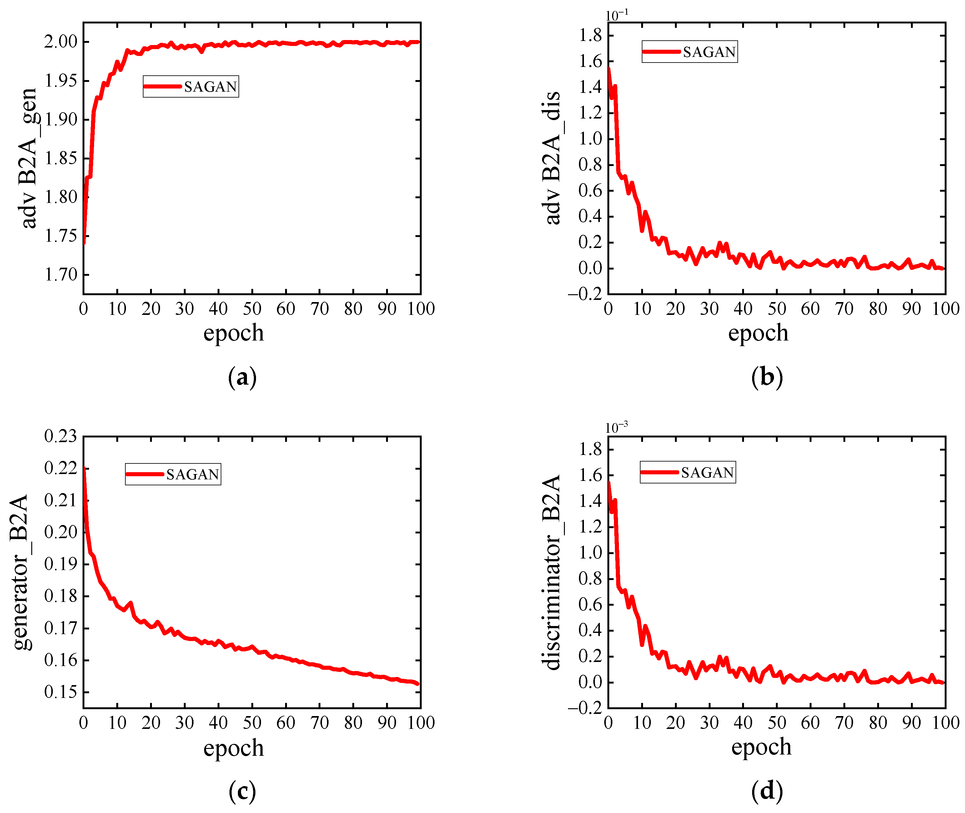
We constructed a training set of 14,416 seismic signals to train the network. The dataset used was the internal dataset of the research group. Firstly, five types of seismic signals with clear information on the event were selected, and then the five large-sized seismic signals were cut to obtain a huge number of seismic signals for the field of seismic exploration. These datasets were used for training, all of which had a size of 256 × 256. These seismic signals include both synthetic seismic signals and field seismic signals. So, the training set is made up of five groups of seismic signals, each of which consists of eight levels of damage. The training set to the validation set to the test set is eight/one/one. To verify the performance of SAGAN, we select the commonly used Wavelet, CNN, and UNet approaches as the comparison methods. In order to better demonstrate the training process, Figure 2 shows the training curves of each process of the SAGAN network. The generator’s adversarial loss function, the discriminator’s adversarial loss function, as well as the generator’s loss function and the discriminator’s loss function together can be seen. Among them, the loss function value of one epoch is obtained by averaging multiple batches of seismic data. The number of epochs used in this experiment is 100, which was verified through multiple interpolation and denoising experiments.

Now, we will give a detailed introduction to the parameter settings during the training process of the SAGAN method. The input size of the network is set to 192 × 192, the size of the inference input is 256 × 256, the training batch size is set to 4, epoch is set from to 0 to 100, and the pre-trained weight models GB2A and DA are loaded. The GB2A model contains 14,776,866 parameters; the DA model contains 9,314,753 parameters. The learning rate of the generator is set to 0.0002, and the learning rate of the discriminator is set to 0.001. The optimizer selects the Adam optimizer; beta1 is 0.5 and beta2 is 0.999. The adversarial loss is the least squares loss. The output of the network is divided into three parts, namely input value, interpolation and denoising value, and label value.

Figure 3 displays the training process of the SAGAN and UNet modules, in which Figure 3a is the curve of PSNR varied with epoch, and Figure 3b is the curve of SSIM varied with epoch. Figure 3a,b demonstrate that the PSNR curves of SAGAN and UNet are both increasing, but the performance of SAGAN is better than that of UNet, and the SSIM curve is also the same. It can be seen that when the number of epochs reaches 100, the curve begins to converge.

The specific steps for reconstructing and denoising experiments using the SAGAN method are as follows:

(1)

Input seismic signals with noise and missing traces into the SAGAN network.

(2)

The input seismic signal is represented in a matrix form, and then the self-attention feature map is obtained through the convolutional feature map decomposition operation of the self-attention mechanism.

(3)

Next, through GAN, we make the seismic signal generated by the generator a fake seismic signal, and the clean seismic signal is true seismic signal. Then, the hyperparameters of the generative adversarial network are iteratively trained and generated.

(4)

Finally, the reconstructed and denoised seismic signal is output.

2.3. The Innovation of SAGAN Method

The incorporation of self-attention modules within convolutions represents a synergy aimed at capturing extensive, multi-level dependencies across various regions within images. Leveraging self-attention empowers the generator to craft images meticulously, orchestrating intricate fine details in each area to harmonize seamlessly with distant portions of the image. Beyond this, the discriminator benefits by imposing intricate geometric constraints more accurately onto the global structure of the image. Consequently, recognizing the potential and applicability of these attributes in seismic signal processing, a tailored SAGAN method has been proposed to optimize the interpolation and denoising processes within this specialized domain.

The selection of UNet, CNN, and Wavelet transform methods for comparison in subsequent experiments stems from their distinct structural and functional attributes. UNet’s architecture stands out for its ability to amalgamate information from diverse receptive fields and scales. However, each layer in UNet, despite its capacity to incorporate varied multi-scale information, operates within limited constraints, primarily focusing on localized information during convolutional operations. Even with different receptive fields, the convolutional unit confines its attention to the immediate neighborhood, overlooking the potential contributions from distant pixels to the current area. In contrast, the inherent capability of the attention mechanism, as incorporated in SAGAN, lies in its aptitude to capture extensive, long-range relationships; factor in global considerations; and synthesize information across multiple scales without confining itself solely to local regions. This stands as a distinctive advantage over methods like UNet, enabling a more holistic perspective when processing seismic signals. Furthermore, the inclusion of CNN serves as a benchmark, representing a classic deep learning methodology. Meanwhile, the utilization of Wavelet transform method adds a classical, traditional approach to the comparative analysis. This diverse selection of methodologies ensures a comprehensive evaluation, juxtaposing modern deep learning techniques with conventional yet established methods, enriching the exploration of seismic signal processing techniques.

3. Interpolation and Denoising Experiments Simultaneously

The seismic signal datasets used in this paper for training, verification, and testing are two-dimensional (2D) synthetic seismic signals, 2D marine seismic signals, three-dimensional (3D) land seismic signals, and 3D field seismic signals. The data sets utilized in this experiment have been sourced from the internal repositories of our research group, ensuring a controlled and specialized collection for our investigations. However, the availability of public data sets plays a pivotal role in advancing research in seismic exploration. Fortunately, repositories like https://wiki.seg.org/wiki/Open_data (accessed on 10 May 2020) offer valuable public data sets, although a standardized, widely accepted public data set remains an ongoing aspiration for scholars within the seismic exploration domain.

The pursuit of a standardized public data set stands as a shared goal among scholars in this field. Such a resource would not only facilitate benchmarking and comparison among various methodologies but also foster collaboration and innovation within the seismic exploration community. As researchers continue to commit their efforts to this pursuit, the creation of a standard public data set remains a collective ambition, promising significant advancements in the field.

In this section, the performance validation of the SAGAN method is undertaken through comprehensive simultaneous interpolation and denoising experiments. The experiments are meticulously divided into four distinct parts, each dedicated to the interpolation and denoising of specific types of seismic signals: 2D synthetic seismic signals, 2D marine seismic signals, 3D land seismic signals, and 3D field seismic signals. This structured approach allows for a comprehensive evaluation of the SAGAN method’s efficacy across diverse seismic signal types, ensuring a robust assessment of its performance in varying signal complexities and domains.

The damage process of seismic signals is divided into two steps. Firstly, Gaussian white noise is artificially added, and the specific method is as follows:

$$y=x+sigma·b$$

(5)

Among them, x is the original seismic signal, b is the added Gaussian white noise, sigma is the variance, also known as noise level, and y is the noisy seismic signal. Because the noise contained in seismic signals is mostly random noise, the method of adding noise is to add Gaussian white noise with different noise levels (variances), just as papers [47,48] also adopt the same strategy.

The second step is to create missing seismic signals. The formation process of missing seismic signals is as follows:

$$y_m=Sy$$

(6)

Among them, S is the sampling matrix, and the damaged seismic signal $y_m$ is obtained by operating the sampling matrix with the noisy signal. This paper sets four sampling rates in the experiment, namely 30%, 40%, 50%, and 60%, which represent the missing rate.

The interpolation and denoising performance metrics are RMSE, PSNR, and SSIM. The definitions of the three metrics are shown in Formulas (7)–(9).

$$\mathrm{RMSE}=\sqrt{\mathrm{MSE}}=\sqrt{\frac{1}{m\times n}{\displaystyle \sum }{\displaystyle \sum }{\left(y_{id}-x\right)}^2}$$

(7)

$$\mathrm{PSNR}=10\times {\log }_{10}\frac{{max}^2\left(x\right)}{\mathrm{MSE}}$$

(8)

$$\mathrm{SSIM}\left(x,y_{id}\right)=\frac{\left(2{\mu }_x{\mu }_{y_{id}}+c_1\right)\left(2{\sigma }_{x{y}_{id}}+c_2\right)}{\left({\mu }_x^2+{\mu }_{y_{id}}^2+c_1\right)\left({\sigma }_x^2+{\sigma }_{y_{id}}^2+c_2\right)}$$

(9)

where $m$ and $n$ are the traces and sampling points of seismic signal, respectively. Among them, the $x$ represents the original seismic signal, $y_{id}$ is the interpolated and denoised seismic signal, ${max}^2\left(x\right)$ is the maximum value in the original seismic signal. ${\mu }_x$ and ${\mu }_{y_{id}}$, respectively, represent the mean of $x$ and $y_{id}$; $c_1$ and $c_2$ are the constants; ${\sigma }_x^2$ and ${\sigma }_{y_{id}}^2$, respectively, represent the variance of $x$ and $y_{id}$; ${\sigma }_{x{y}_{id}}$ represents $x$ and $y_{id}$ covariance.

The smaller the value of RMSE, the better the interpolation and denoising effect. The higher the value of PSNR, the better the interpolation and denoising effect. The closer the value of SSIM is to 1, the better the interpolation and denoising effect. When the MSE value approaches 0, the PSNR value tends to infinity, but this situation is almost impossible to achieve.

3.1. Two-Dimensional Synthetic Seismic Signal Interpolation and Denoising

In the experimental setup, a 2D synthetic seismic signal is intentionally subjected to varying degrees of damage, encompassing eight distinct levels of impairment. Specifically, these levels are delineated by two factors: a noise level of 10 or 20, coupled with different sampling rates (30%, 40%, 50%, 60%). This controlled setting aims to simulate diverse scenarios of signal degradation. To restore and denoise these impaired seismic signals, the Wavelet, CNN, UNet, and SAGAN methods are employed. The results of the signal recovery across all eight damage degrees are presented in Figure 4 and subsequent displays, providing a comprehensive visual representation of the recovery outcomes for each scenario. Figure 4a showcases the pristine state of the 2D synthetic seismic signal—a clean representation comprising three distinct events. This signal is characterized by 256 traces, each containing 256 sampling points, forming the foundational basis for the subsequent comparative analyses of signal restoration and denoising efficacy.

Upon scrutinizing the subgraphs of Figure 4, a notable observation arises. Specifically, in Figure 4k, where the noise level is set at 10 and the missing rate at 30%, a discernible discrepancy surfaces: the error map derived from the SAGAN method displays minimal residuals, contrasting starkly with the conspicuous residual evident in the error map generated by the Wavelet transform method across three events. Delving deeper into Figure 4m,o, a compelling trend emerges: with the consistent missing rate, the escalation in noise levels indeed exerts a tangible influence on both interpolation and denoising outcomes. Of note, the impact is discernable as the missing rate ascends; the performance of CNN gradually deteriorates in its efficacy for interpolation and denoising. In stark contrast, SAGAN exhibits a consistent ability to sustain continuity amidst escalating missing rates, underscoring its resilience in preserving continuous events.

Observations from Figure 4 elucidate a crucial aspect: at a 60% degree of missingness, the method exhibits certain limitations attributed to substantial contiguous missing regions. Nonetheless, it is notable that in most instances, the method proposed in this manuscript excels in simultaneous interpolation and denoising. Furthermore, the efficacy of SAGAN becomes evident, particularly as the extent of damage intensifies, owing to its adaptive utilization of the attention mechanism in recovering seismic signals. To better discern the recovery performance across the four approaches,

Table 1. Performance metrics of different approaches for interpolation and denoising of 2D synthetic seismic signal.

RMSE/PSNR (dB)/SSIM
Level of Damage	Input PSNR (dB)	Methods
		Wavelet	CNN	UNet	SAGAN
Noise Sigma = 10, Missing rate = 30%	21.3675	0.0373/28.5560/0.9466	0.0193/34.2746/0.9553	0.0093/40.6373/0.9900	0.0100/40.0055/0.9881
Noise Sigma = 10, Missing rate = 40%	20.5388	0.0471/26.5555/0.9389	0.0281/31.0139/0.9504	0.0134/37.5471/0.9888	0.0169/35.5634/0.9854
Noise Sigma = 10, Missing rate = 50%	19.2951	0.0693/23.1836/0.9355	0.0469/26.5850/0.9463	0.0205/34.1264/0.9759	0.0141/36.7690/0.9851
Noise Sigma = 10, Missing rate = 60%	20.3152	0.0453/26.8821/0.9497	0.0238/32.4514/0.9623	0.0220/33.1525/0.9731	0.0171/35.3238/0.9821
Noise Sigma = 20, Missing rate = 30%	17.8284	0.1063/19.4569/0.8822	0.0677/23.3855/0.9078	0.0233/32.7898/0.9684	0.0137/36.8497/0.9693
Noise Sigma = 20, Missing rate = 40%	14.7681	0.1643/15.6867/0.8541	0.1306/17.6812/0.8280	0.0317/30.7922/0.9709	0.0229/32.9653/0.9711
Noise Sigma = 20, Missing rate = 50%	17.9899	0.0962/20.3390/0.8825	0.0563/24.9824/0.9105	0.0358/29.2340/0.9741	0.0182/35.1373/0.9760
Noise Sigma = 20, Missing rate = 60%	17.0659	0.0965/20.3090/0.8816	0.0566/24.9474/0.9186	0.0363/28.8516/0.9648	0.0179/35.2176/0.9665

Bold PSNR and SSIM values indicate the maximum value, while bold RMSE values indicate the minimum value.

encapsulates the RMSE, PSNR, and SSIM values. These metrics aim to provide a comprehensive evaluation framework, allowing a nuanced comparison of the performance among these methodologies.

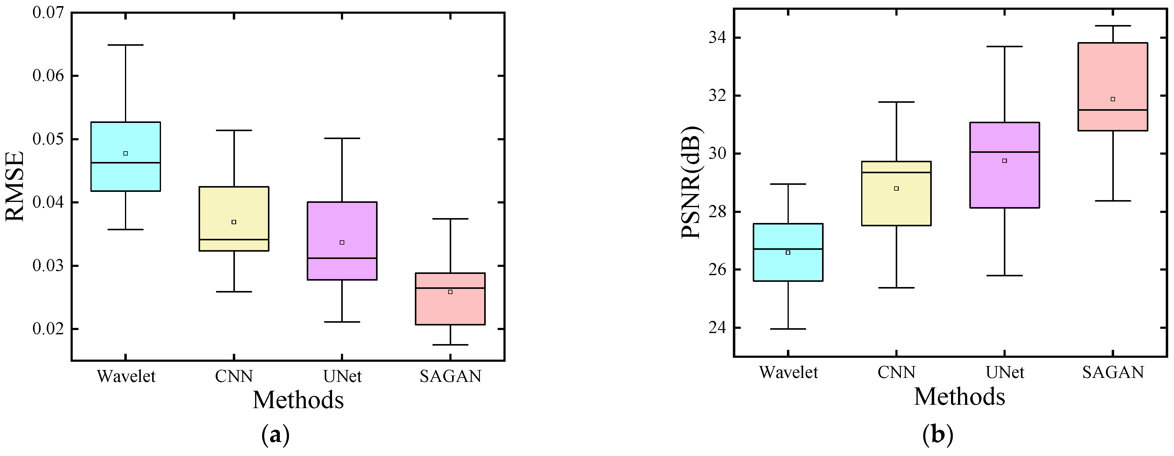
From the data in Table 1, it becomes apparent that at specific conditions, such as a noise level of 10 and a missing rate of 30% or a noise level of 10 with a missing rate of 40%, the recovery efficacy of UNet surpasses that of SAGAN. However, as the extent of damage escalates, SAGAN exhibits its strengths and advantages over UNet. To enhance the visual representation of these results, we organized the RMSE and PSNR values from Table 1 into box plots for improved visualization. Figure 5 comprises two distinct box plots, delineating pertinent insights. Notably, in Figure 5a, the median line representing the SAGAN method sits below that of the comparative method, highlighting SAGAN’s superior performance. Conversely, in Figure 5b, the median line for the SAGAN method exceeds that of the comparative method, indicating a differing trend in performance under these specific conditions.

3.2. Two-Dimensional Marine Seismic Signal Interpolation and Denoising

In the realm of the 2D marine seismic signal, diverse damage degrees were intentionally induced, spanning eight distinct levels. Each setting included variations in the noise level, set at 10 or 20, and diverse sampling rates ranging from 30% to 60%. Employing the Wavelet, CNN, UNet, and SAGAN methods, the seismic signal underwent a process of interpolation and denoising. Figure 6 aptly illustrates the resulting recovery outcomes across varying sampling rates. Figure 6a serves as a visual depiction of the original 2D marine seismic signal. This intricate signal comprises multiple discernible events, with a trace number totaling 256 and 256 sampling points, encapsulating the complexity inherent in such seismic signals.

In Figure 6m, a notable observation emerges: the error map derived from the Wavelet transform method exhibits the most pronounced residuals. Notably, on distinct seismic traces, the performance of SAGAN outshines that of UNet and CNN, showcasing superior error reduction. Continuing the observation with Figure 6n, it becomes apparent that when confronted with consecutively missing traces, the efficacy of various methods in reconstructing the seismic signal presents challenges. Portions of the missing trace remain unreconstructed across methodologies. However, even under these demanding conditions, the interpolation and denoising outcomes achieved by SAGAN maintain a noticeable superiority over other methodologies.

In scrutinizing Figure 6, a discernible trend emerges: when confronted with lower damage degrees, both methods exhibit commendable restoration of the seismic signal. However, as the damage degree escalates, the advantage of SAGAN becomes increasingly pronounced. SAGAN’s adept use of adaptive attention mechanisms enables a more discerning observation of events within seismic signals, facilitating more effective recovery. This characteristic positions SAGAN as a superior choice for seismic signal interpolation and denoising when compared to Wavelet, CNN, and UNet. To facilitate a clearer comparison of the recovery effects among the four approaches,

Table 2. Performance metrics of interpolation and denoising of 2D marine seismic signal by different approaches.

RMSE/PSNR (dB)/SSIM
Level of Damage	Input PSNR (dB)	Methods
		Wavelet	CNN	UNet	SAGAN
Noise Sigma = 10, Missing rate = 30%	23.0118	0.0557/25.0762/0.8756	0.0328/29.6861/0.9229	0.0295/30.5934/0.9527	0.0272/31.3150/0.9557
Noise Sigma = 10, Missing rate = 40%	22.1721	0.0598/24.4692/0.8312	0.0381/28.3798/0.8999	0.0274/31.1412/0.9453	0.0257/31.6912/0.9504
Noise Sigma = 10, Missing rate = 50%	21.1377	0.0692/23.2014/0.8010	0.0437/27.1964/0.8703	0.0403/27.7319/0.9296	0.0316/29.9147/0.9343
Noise Sigma = 10, Missing rate = 60%	20.1712	0.0808/21.8555/0.7571	0.0551/25.1781/0.8319	0.0765/22.6639/0.8776	0.0497/26.0973/0.8937
Noise Sigma = 20, Missing rate = 30%	22.5951	0.0564/24.9794/0.8346	0.0356/28.9685/0.8887	0.0337/29.4952/0.9083	0.0321/29.8710/0.9168
Noise Sigma = 20, Missing rate = 40%	21.7344	0.0643/23.8343/0.7926	0.0423/27.4818/0.8626	0.0408/27.7084/0.8910	0.0297/30.5528/0.9085
Noise Sigma = 20, Missing rate = 50%	20.1474	0.0836/21.5574/0.7734	0.0553/25.1522/0.8513	0.0546/25.1785/0.8731	0.0473/26.4918/0.8896
Noise Sigma = 20, Missing rate = 60%	19.4090	0.0941/20.5252/0.7284	0.0704/23.0576/0.8090	0.0893/20.9284/0.8413	0.0615/24.3725/0.8504

Bold PSNR and SSIM values indicate the maximum value, while bold RMSE values indicate the minimum value.

compiles the RMSE, PSNR, and SSIM values. These metrics serve as quantitative indicators to discern and evaluate the performance discrepancies across these methodologies.

The data in Table 2 reveal a pertinent trend: at lower damage degrees in the seismic signal, the PSNR and SSIM values of SAGAN only marginally exceed those of UNet. However, as the damage degree intensifies, SAGAN consistently outperforms UNet, aligning with our prior theoretical analysis. Figure 7 presents two box plots, offering additional insights. In Figure 7a, the median line representing the SAGAN method sits below that of the UNet, CNN, and Wavelet methods, indicative of its slightly lower performance in specific conditions. Conversely, in Figure 7b, the median line for the SAGAN method surpasses that of the UNet, CNN, and Wavelet methods, signaling its superior performance under these circumstances. These visualizations further corroborate the performance disparities across methodologies under varying degrees of damage in seismic signals.

Aimed at better proving the performance of SAGAN, the 3D seismic signals are recovered below.

3.3. Three-Dimensional Land Seismic Signal Interpolation and Denoising

The investigation extends ablation experiments initially conducted in a 2D setting to encompass the dynamic scope of 3D land and field seismic signals. To delineate the impact of varied damage intensities, the 3D land seismic signals were subjected to eight distinct damage degrees. Specifically, these degrees were configured with two noise levels, 10 and 20, encompassing sampling rates of 30%, 40%, 50%, and 60% for each noise level. Employing the Wavelet, CNN, UNet, and SAGAN methodologies, the seismic signals underwent interpolation and denoising procedures. As illustrated in Figure 8, the outcomes of the recovery process under different sampling rates are depicted. Figure 8a specifically presents the original 3D land seismic signal, comprising a multitude of events within its slice. This slice encompasses 256 traces with a sampling point of 256, manifesting the intricacies inherent in the seismic signal.

Figure 8l distinctly highlights the discernible presence of artifacts, particularly evident when employing the UNet method. This observation underscores the inherent challenges encountered during the intricate process of reconstructing and denoising three-dimensional seismic signals. Analogous to their two-dimensional counterparts, the complexity amplifies when confronted with uninterrupted missing traces. However, the culmination of comprehensive experimentation and comparative analysis among various methodologies unequivocally demonstrates that the SAGAN method excels in achieving optimal interpolation efficacy.

Observing Figure 8, it becomes apparent that for lower degrees of damage, both methods demonstrate a proficient restoration of the seismic signal. However, as the damage escalates, the advantage in recovery effectiveness distinctly tilts in favor of the SAGAN approach. This disparity arises due to SAGAN’s adaptive utilization of attention mechanisms, specifically tailored to the recovery of seismic signals. A mere visual analysis of the recovery outcome graphs fails to comprehensively elucidate the nuanced efficacy of distinct methods. To more precisely discern the recovery effects of the four approaches,

Table 3. Performance metrics of different approaches for interpolation and denoising of 3D land seismic signal.

RMSE/PSNR (dB)/SSIM
Level of Damage	Input PSNR (dB)	Methods
		Wavelet	CNN	UNet	SAGAN
Noise Sigma = 10, Missing rate = 30%	20.9503	0.0446/27.0192/0.8923	0.0337/29.4459/0.9271	0.0271/31.4718/0.9372	0.0197/34.0409/0.9401
Noise Sigma = 10, Missing rate = 40%	21.9238	0.0357/28.9480/0.8904	0.0259/31.7807/0.9249	0.0211/33.6977/0.9292	0.0175/34.4111/0.9364
Noise Sigma = 10, Missing rate = 50%	20.5418	0.0408/27.7935/0.8809	0.0333/29.5581/0.9156	0.0284/30.6753/0.9210	0.0216/33.6023/0.9307
Noise Sigma = 10, Missing rate = 60%	20.0212	0.0479/26.3989/0.8565	0.0356/28.9566/0.9062	0.0321/29.7350/0.9184	0.0299/30.4670/0.9211
Noise Sigma = 20, Missing rate = 30%	21.5883	0.0428/27.3807/0.8319	0.0314/29.8987/0.8990	0.0303/30.3749/0.8955	0.0256/31.8639/0.9006
Noise Sigma = 20, Missing rate = 40%	21.1568	0.0482/26.3428/0.8209	0.0345/29.2482/0.8752	0.0326/29.6741/0.8929	0.0273/31.1526/0.8932
Noise Sigma = 20, Missing rate = 50%	20.9307	0.0571/24.8710/0.8165	0.0493/26.0855/0.8531	0.0475/26.5899/0.8850	0.0278/31.1129/0.8861
Noise Sigma =20, Missing rate = 60%	19.8891	0.0649/23.9510/0.8105	0.0514/25.3785/0.8360	0.0501/25.7908/0.8651	0.0374/28.3685/0.8752

Bold PSNR and SSIM values indicate the maximum value, while bold RMSE values indicate the minimum value.

meticulously presents the RMSE, PSNR, and SSIM values corresponding to each methodology.

Table 3 distinctly portrays a substantial disparity in the PSNR and SSIM values, showcasing the marked superiority of SAGAN over the UNet, CNN, and Wavelet methods. Notably, this pronounced performance divergence persists consistently when the missing rate of the seismic signal stands at 50%, irrespective of the noise level. Even at a missing rate of 60%, SAGAN retains a notable edge in the recovery process, aligning with the anticipated outcomes derived from theoretical analysis. These objective performance metrics, thus, validate and reinforce the empirical findings, affirming the advantageous proficiency of the SAGAN methodology in seismic signal recovery.

Figure 9 shows two box plots, and it can be observed that the median line of the SAGAN method in Figure 9a is lower than that of the comparison method, while the median line of the SAGAN method in Figure 9b is higher than that of the comparison method.

The culminating segment of the experimentation process involves the recovery of the 3D field seismic signal, presenting the most formidable challenge within this experimental phase.

3.4. Three-Dimensional Field Seismic Signal Interpolation and Denoising

The intricate nature of 3D field seismic signals necessitates comprehensive efforts in their interpolation and denoising processes. To address this challenge, various damage levels were meticulously assigned to the 3D field seismic signal, encompassing eight distinct degrees. These levels were carefully structured around two noise levels, 10 and 20, coupled with sampling rates set at 30%, 40%, 50%, and 60%. Interpolation and denoising endeavors were meticulously conducted, employing the Wavelet, CNN, UNet, and SAGAN methodologies, each method tailored to address the complexities inherent in these seismic signals. In Figure 10, the interpolation and denoising results under diverse sampling rates are shown. Figure 10a shows the original 3D field seismic signal. The 3D field seismic signal slice consists of complex events; the trace number in this seismic signal is 256, and the sampling point is 256.

A discernible trend emerges from Figure 10k,o, highlighting that at a missing rate of 30%, multiple methodologies exhibit superior efficacy in reconstructing seismic signals. However, as the missing rate escalates to 40%, 50%, and 60%, the effectiveness of interpolation gradually diminishes across the methods. Notwithstanding, amidst these escalating missing rates, the SAGAN method consistently maintains its superior performance in both interpolation and denoising, outperforming its counterparts. Notably, a keen observation from Figure 10m,q reveals that heightened noise levels predominantly impact the inclined events within the seismic signal. Specifically, at a noise level of 20, there is a discernible increase in residual tilted events, signifying the nuanced impact of noise amplification on the intricate components of the seismic data.

Figure 10 presents a comprehensive overview, indicating that all methods demonstrate a foundational capacity to undertake the intricate tasks of reconstructing and denoising seismic signals. Nevertheless, the distinctive advantage of SAGAN becomes evident, particularly in handling seismic signals plagued by higher missing rates, showcasing its superior recovery performance in such scenarios. These nuances are further validated through the RMSE, PSNR, and SSIM values meticulously presented in

Table 4. Performance metrics of different methods for interpolation and denoising of 3D field seismic signal.

RMSE/PSNR (dB)/SSIM
Level of Damage	Input PSNR (dB)	Methods
		Wavelet	CNN	UNet	SAGAN
Noise Sigma = 10, Missing rate = 30%	22.7847	0.0386/28.2574/0.8834	0.0323/30.1905/0.9354	0.0316/30.7552/0.9489	0.0271/31.3864/0.9510
Noise Sigma = 10, Missing rate = 40%	21.0973	0.0416/27.6109/0.8598	0.0329/29.6443/0.9133	0.0313/31.0183/0.9291	0.0251/31.6970/0.9354
Noise Sigma = 10, Missing rate = 50%	20.1610	0.0478/26.4200/0.8366	0.0371/28.6065/0.8962	0.0335/29.5323/0.9122	0.0315/30.8083/0.9198
Noise Sigma = 10, Missing rate = 60%	19.9425	0.0550/25.1950/0.7960	0.0434/27.3696/0.8611	0.0415/27.6118/0.8633	0.0369/28.4234/0.8774
Noise Sigma = 20, Missing rate = 30%	20.7421	0.0417/27.6082/0.8468	0.0353/29.0379/0.8840	0.0341/29.3687/0.8994	0.0320/30.5377/0.9090
Noise Sigma = 20, Missing rate = 40%	20.3006	0.0471/26.6099/0.8235	0.0391/28.1603/0.8644	0.0380/28.4072/0.8800	0.0342/29.3154/0.8918
Noise Sigma = 20, Missing rate = 50%	19.4386	0.0496/26.0866/0.8037	0.0469/26.8474/0.8473	0.0443/27.0646/0.8591	0.0366/28.5873/0.8745
Noise Sigma = 20, Missing rate = 60%	18.2866	0.0613/24.2482/0.7591	0.0577/24.7718/0.8094	0.0517/25.5704/0.8112	0.0473/26.5031/0.8298

Bold PSNR and SSIM values indicate the maximum value, while bold RMSE values indicate the minimum value.

. Additionally, Figure 11, depicted through two box plots, accentuates these disparities; in Figure 11a, the median line attributed to the SAGAN method conspicuously rests below those of the UNet, CNN, and Wavelet methodologies. Conversely, in Figure 11b, the median line associated with the SAGAN method notably surpasses those of the comparative UNet, CNN, and Wavelet methods. These visual representations offer compelling evidence supporting the pronounced advantages of the SAGAN approach in effectively handling seismic signal recovery across diverse conditions.

Table 4 demonstrates that the performance indexes of the SAGAN method are not as advantageous as when recovering synthetic seismic signals, which indicates that all methods can recover seismic signals better in the actual seismic signal recovery task. However, in order that pursue high-quality seismic signals to achieve better results in subsequent seismic signal interpretation tasks, the SAGAN method has obvious advantages for both 2D and 3D seismic signal recovery.

The above four experimental results all indicate that the objective performance metrics of the SAGAN method have significant advantages. However, we cannot simply focus on subjective interpolation and denoising maps or only look at objective performance metrics. We should also combine subjective and objective factors to better illustrate the generalization of the method. Due to the fact that high-quality seismic signals are provided for geologists to better interpret the corresponding seismic signals, subjective maps are also very crucial. We can find that in the above experiments, the subjective maps of the SAGAN method are also the clearest among the four methods in terms of preserving events of the original seismic signals.

3.5. Interpolation Experiments with Various Noises

Next, we add two types of noise to the 3D field seismic signal, namely colored noise and Gaussian white noise. These two types of noise are also common noises in seismic signals. The above interpolation and denoising experiments are then repeated using different methods. In order to simplify the layout, Figure 12 only shows the added noise and does not show the interpolation and denoising results of different methods.

Table 5. Performance metrics of different methods for interpolation and denoising of 3D field seismic signal (two types of noise, colored noise and Gaussian white noise).

RMSE/PSNR (dB)/SSIM
Level of Damage	Input PSNR (dB)	Methods
		Wavelet	CNN	UNet	SAGAN
Noise Sigma = 10, Missing rate = 30%	22.5773	0.0548/25.2281/0.8662	0.0487/26.2430/0.9123	0.0441/27.1179/0.9439	0.0428/27.3644/0.9472
Noise Sigma = 10, Missing rate = 40%	21.7290	0.0444/27.0572/0.8471	0.0359/28.8922/0.8795	0.0285/30.8965/0.9278	0.0271/31.3498/0.9316
Noise Sigma = 10, Missing rate = 50%	19.8068	0.0592/24.5546/0.8236	0.0536/25.4214/0.8581	0.0404/27.8755/0.9112	0.0386/28.2744/0.9147
Noise Sigma = 10, Missing rate = 60%	18.7340	0.0730/22.7289/0.7854	0.0682/23.3302/0.8128	0.0558/25.0681/0.8606	0.0540/25.3595/0.8670
Noise Sigma = 20, Missing rate = 30%	20.4312	0.0520/25.6809/0.8152	0.0483/26.3186/0.8644	0.0374/28.5391/0.9044	0.0341/29.3532/0.9082
Noise Sigma = 20, Missing rate = 40%	19.2761	0.0670/23.4765/0.7867	0.0647/23.7855/0.8319	0.0530/25.5068/0.8777	0.0494/26.1325/0.8818
Noise Sigma = 20, Missing rate = 50%	19.9476	0.0554/25.1360/0.7662	0.0478/26.4057/0.8146	0.0403/27.8943/0.8586	0.0385/28.3012/0.8638
Noise Sigma = 20, Missing rate = 60%	18.1415	0.0815/21.7775/0.7298	0.0757/22.4228/0.7669	0.0666/23.5253/0.8088	0.0627/24.0545/0.8166

Bold PSNR and SSIM values indicate the maximum value, while bold RMSE values indicate the minimum value.

still gives the performance indicators.

It can be seen in Table 5 that after adding two kinds of noise, the performance index of the SAGAN method is the best regardless of the missing rate, which once again verifies the advantages of multi-scale SAGAN.

Finally, we increase the intensity of the colored noise and continue the interpolation and denoising experiments of 3D field seismic signals. The added noise images are shown in Figure 13.

Table 6. Performance metrics of different methods for interpolation and denoising of 3D field seismic signal (two types of noise: 1.5 times colored noise and Gaussian white noise).

RMSE/PSNR (dB)/SSIM
Level of Damage	Input PSNR (dB)	Methods
		Wavelet	CNN	UNet	SAGAN
Noise Sigma = 10, Missing rate = 30%	22.0255	0.0448/26.9825/0.8717	0.0298/30.5137/0.9230	0.0257/31.8075/0.9486	0.0243/32.2854/0.9510
Noise Sigma = 10, Missing rate = 40%	21.5153	0.0455/26.8411/0.8488	0.0320/29.9029/0.9028	0.0278/31.1314/0.9303	0.0266/31.4957/0.9337
Noise Sigma = 10, Missing rate = 50%	21.1320	0.0515/25.7713/0.8215	0.0435/27.2209/0.8813	0.0377/28.4815/0.9107	0.0372/28.5929/0.9150
Noise Sigma = 10, Missing rate = 60%	19.3804	0.0633/23.9739/0.7852	0.0536/25.4209/0.7941	0.0473/26.4952/0.8595	0.0455/26.8333/0.8675
Noise Sigma = 20, Missing rate = 30%	20.8084	0.0479/26.4002/0.8108	0.0450/26.9311/0.8462	0.0326/29.7242/0.9032	0.0309/30.1913/0.9069
Noise Sigma = 20, Missing rate = 40%	19.1098	0.0698/23.1276/0.7883	0.0666/23.5263/0.8447	0.0558/25.0684/0.8771	0.0517/25.7297/0.8828
Noise Sigma = 20, Missing rate = 50%	19.1150	0.0645/23.8054/0.7717	0.0582/24.7030/0.8337	0.0489/26.2195/0.8626	0.0450/26.9295/0.8664
Noise Sigma = 20, Missing rate = 60%	19.1768	0.0661/23.5939/0.7270	0.0595/24.3124/0.7856	0.0528/25.5430/0.8063	0.0498/26.0576/0.8146

Bold PSNR and SSIM values indicate the maximum value, while bold RMSE values indicate the minimum value.

lists the performance indicators of seismic signal interpolation and denoising using different methods under different circumstances.

Observing Figure 13 and analyzing Table 6, it can be found that when 1.5 times the colored noise is added and the Gaussian noise level is 10, the superposition of the two noises may produce a neutralizing effect, which will weaken the overall noise. The performance metrics after interpolation and denoising will generally be better than without colored noise. However, when the noise level is 20, the overall effect is not as good as when there is only Gaussian noise, which proves that when multiple noises coexist, the difficulty of interpolation and denoising will increase. Overall, the proposed SAGAN method still has advantages.

3.6. Comparison of Running Times of Different Methods

In the last part of the experiments, we started to analyze the computational efficiency to see what the testing time of different methods is while ensuring the accuracy of interpolation and denoising. If the test time is also an advantage, then sacrificing a lot of training time is worth it.

Table 7. The running time of different methods for interpolating and denoising different seismic signals.

Types of Seismic Signals	Wavelet	CNN	UNet	SAGAN
2D synthetic seismic signal	4.13 s	4.33 s	2.72 s	2.64 s
2D marine seismic signal	4.59 s	4.64 s	3.12 s	3.04 s
3D land seismic signal	4.18 s	4.81 s	2.96 s	2.80 s
3D field seismic signal	4.94 s	4.04 s	3.28 s	2.88 s

lists the running time results after using different methods to interpolate and denoise different types of seismic signals.

We analyze the data in Table 7. For the two-dimensional synthetic seismic signal, the running time of Wavelet transform is 4.13 s, which increases by 4.8% for CNN, decreases by 34.1% for UNet, and decreases by 36.1% for SAGAN. Compared with UNet, SAGAN dropped by 2.9%. For a three-dimensional field seismic signal, the Wavelet transform time is 4.94 s. Compared with Wavelet transform, the CNN running time is reduced by 18.2%, the UNet running time is reduced by 33.6%, and the SAGAN running time is reduced by 41.7%. Compared with UNet, the running time of SAGAN is reduced by 12.2%. It can be found from Table 5 that although the deep learning methods require a lot of time to train network parameters in the early stage, when the network training is completed, the test time has an advantage compared with the traditional methods, and the interpolation and denoising accuracy has also been improved. Therefore, deep learning methods have attracted more and more attention from scholars in the field of seismic signal processing. Each method has its own unique contribution to seismic signal processing and has accelerated the intelligent development of seismic exploration.

4. Conclusions

The acquisition process of seismic signals is notably susceptible to incompleteness and noise, influenced by both the exploration environment and equipment. Recent years have witnessed an expanding realm of research delving into the application of deep learning in seismic signal processing, yielding commendable outcomes. Consequently, this paper delves into the simultaneous interpolation and denoising of seismic signals, amalgamating the prowess of self-attention and generative adversarial networks. The pivotal contribution of this manuscript lies in the formulation of the multi-scale SAGAN method. This method breaks free from the constraints of local areas, effectively broadening the receptive field and synthesizing information across varied scales. By employing this innovative approach, the multi-scale SAGAN method facilitates the concurrent interpolation and denoising of seismic signals, thereby significantly bolstering operational efficiency in signal processing methodologies. This advancement heralds a promising stride towards enhancing the efficacy of seismic data handling in complex exploration environments. The primary conclusions of the content are as follows:

(1)

With a view to intelligentize seismic signal processing, the simultaneous interpolation and denoising of seismic signals are studied. The Wavelet, CNN, UNet, and proposed SAGAN methods are selected to conduct four sets of comparative experiments. These two methods are used to reconstruct and denoise 2D synthetic seismic signals with different damage degrees and then apply them to 2D marine seismic signals. Assessing the PSNR metrics in the realm of two-dimensional synthetic seismic signal experimentation reveals compelling insights. The SAGAN method, in comparison to Wavelet, demonstrates an average enhancement of 59.05%, while when juxtaposed with CNN and UNet, it showcases average improvements of 33.68% and 7.75%, respectively. This substantial margin signifies the pronounced efficacy of the SAGAN approach in elevating the quality of synthetic seismic signal interpolation. Shifting the focus to the domain of two-dimensional marine seismic signals, the SAGAN method maintains a commendable performance. In this context, its average improvements over Wavelet, CNN, and UNet stand at 24.16%, 7.07%, and 6.90%, respectively. Despite a slightly moderated advantage, the SAGAN method still outshines other methodologies, affirming its consistent proficiency in enhancing the quality of marine seismic signal interpolation.

(2)

Furthermore, 3D land seismic signals and field seismic signals are reconstructed and denoised. Four sets of comparative experiments show the performance of SAGAN. That is, compared with Wavelet, CNN, and UNet, SAGAN has the best interpolation and denoising performance. In addition, the recovered seismic signal is also smoother and more continuous, without faulting. Judging from the PSNR metrics of the three-dimensional synthetic seismic signal experiment, the SAGAN method has an average improvement of 19.89% compared to Wavelet, an average improvement of 10.71% compared to CNN, and an average improvement of 7.15% compared to UNet. From the perspective of three-dimensional field seismic signals, the SAGAN method has an average improvement of 11.90%, 5.62%, and 3.46% compared to Wavelet, CNN, and Unet, respectively. These show that 3D seismic signal interpolation and denoising are indeed difficult.

(3)

In the process of training the network, we found that the training performance of SAGAN will be limited by the training set and batch size, and how to better self-adapt to the tasks of seismic signal interpolation and denoising and achieve better performance is the focus of our following research in the future.

References

- Chang, W.; McMechan, G. 3D acoustic prestack reverse-time migration. Geophys. Prospect. 1990, 38, 737–755. [Google Scholar] [CrossRef]
- Virieux, J.; Operto, S. An overview of full-waveform inversion in exploration geophysics. Geophysics 2009, 74, WCC1–WCC26. [Google Scholar] [CrossRef]
- Verschuur, D.; Berkhout, A.; Wapenaar, C. Adaptive surface-related multiple elimination. Geophysics 1992, 57, 1166–1177. [Google Scholar] [CrossRef]
- Zwartjes, P.; Gisolf, A. Fourier reconstruction of marine-streamer data in four spatial coordinates. Geophysics 2006, 71, V171–V186. [Google Scholar] [CrossRef]
- Dario, A.; Rodrigo, S.; Reinaldo, S.; Emilio, V. Interpolating seismic data with conditional generative adversarial networks. IEEE Geosci. Remote Sens. Lett. 2018, 15, 1952–1956. [Google Scholar]
- Li, Y.; Wang, J.; Li, H.; Ren, P. Peak Colocalized Orthogonal Matching Pursuit for Seismic Trace Decomposition. IEEE Access 2020, 8, 8620–8626. [Google Scholar] [CrossRef]
- Zhang, X.; Zhang, S.; Lin, J.; Sun, F.; Zhu, X.; Yang, Y.; Tong, X.; Yang, H. An efficient seismic data acquisition based on compressed sensing architecture with generative adversarial networks. IEEE Access 2019, 7, 105948–105961. [Google Scholar] [CrossRef]
- Hindriks, K.; Duijndam, A. Reconstruction of 3-D seismic signals irregularly sampled along two spatial coordinates. Geophysics 1999, 65, 253–263. [Google Scholar] [CrossRef]
- Satish, S.; Partha, S.; Phil, D.; John, P. Spectral decomposition of seismic data with continuous-wavelet transform. Geophysics 2005, 70, 19–25. [Google Scholar]
- Jones, I.; Levy, S. Signal-to-noise ratio enhancement in multichannel seismic data via the Karhunen-Loéve transform. Geophys. Prospect. 1987, 35, 12–32. [Google Scholar] [CrossRef]
- Liu, D.; Wang, W.; Wang, X.; Wang, C.; Pei, J. Poststack seismic data denoising based on 3-D convolutional neural network. IEEE Trans. Geosci. Remote Sens. 2020, 58, 1598–1629. [Google Scholar] [CrossRef]
- Kundu, A.; Bhadauria, Y.; Basu, S.; Mukhopadhyay, S. Application of ANN and SVM for identification of tsunamigenic earthquakes from 3-component seismic data. In Proceedings of the IEEE International Conference on Recent Trends in Electronics, Information & Communication Technology, Bangalore, India, 19–20 May 2017; pp. 10–13. [Google Scholar]
- Kunihiko, F. Neocognitron: A self-organizing neural network model for a mechanism of pattern recognition unaffected by shift in position. Biol. Cybern. 1980, 36, 193–202. [Google Scholar]
- Dong, C.; Loy, C.; He, K. Image super-resolution using deep convolutional networks. IEEE Trans. Pattern Anal. Mach. Intell. 2016, 38, 295–307. [Google Scholar] [CrossRef] [PubMed]
- Mandelli, S.; Borra, F.; Lipari, V.; Bestagini, P.; Sarti, A.; Tubaro, S. Seismic data interpolation through convolutional autoencoder. In SEG Technical Program Expanded Abstracts; SEG: Houston, TX, USA, 2018; pp. 4101–4105. [Google Scholar]
- Park, J.; Yoon, D.; Seol, S. Reconstruction of seismic field data with convolutional U-Net considering the optimal training input data. In SEG Technical Program Expanded Abstracts; SEG: Houston, TX, USA, 2019. [Google Scholar]
- Wang, Y.; Wang, B.; Tu, N. Seismic Trace Interpolation for Irregularly Spatial Sampled Data Using Convolutional Auto-Encoder. Geophysics 2020, 85, V119–V130. [Google Scholar] [CrossRef]
- Gao, Y.; Zhang, W. Robust recovery of a kind of weighted l1-minimization without noise level. Int. J. Wavelets Multiresolut. Inf. Process. 2022, 20, 2250012. [Google Scholar] [CrossRef]
- Wang, B.; Zhang, N.; Lu, W.; Zhang, P.; Geng, J. Seismic Data Interpolation Using Deep Learning Based Residual Networks. In Proceedings of the 80th EAGE Conference and Exhibition, Copenhagen, Denmark, 11–14 June 2018. [Google Scholar]
- Jin, Y.; Wu, X.; Chen, J.; Han, Z.; Hu, W. Seismic data denoising by deep-residual networks. In SEG Technical Program Expanded Abstracts; SEG: Houston, TX, USA, 2018; pp. 4593–4597. [Google Scholar]
- Siahkoohi, A.; Kumar, R.; Herrmann, F. Seismic Data Reconstruction with Generative Adversarial Networks. In Proceedings of the 80th EAGE Conference and Exhibition, Copenhagen, Denmark, 11–14 June 2018. [Google Scholar]
- Dodda, V.; Kuruguntla, L.; Mandpura, A.; Elumalai, K. Simultaneous seismic data denoising and reconstruction with attention-based wavelet-convolutional neural network. IEEE Trans. Geosci. Remote Sens. 2023, 61, 5908814. [Google Scholar] [CrossRef]
- Li, C.; Wen, X.; Liu, X.; Zu, S. Simultaneous seismic data interpolation and denoising based on nonsubsampled contourlet transform integrating with two-step iterative log thresholding algorithm. IEEE Trans. Geosci. Remote Sens. 2023, 60, 5918210. [Google Scholar] [CrossRef]
- Cao, J.; Cai, Z.; Liang, W. A novel thresholding method for simultaneous seismic data reconstruction and denoising. J. Appl. Geophys. 2020, 177, 104027. [Google Scholar] [CrossRef]
- Iqbal, N. DeepSeg: Deep Segmental Denoising Neural Network for Seismic Data. IEEE Trans. Neural Netw. Learn. Syst. 2023, 34, 3397–3404. [Google Scholar] [CrossRef]
- Zhang, C.; Baan, M. Microseismic Signal Reconstruction from Strong Complex Noise Using Low-Rank Structure Extraction and Dual Convolutional Neural Networks. IEEE Trans. Neural Netw. Learn. Syst. 2023; early access. [Google Scholar] [CrossRef]
- Bahdanau, D.; Cho, K.; Bengio, Y. Neural machine translation by jointly learning to align and translate. arXiv 2014, arXiv:1409.0473. [Google Scholar]
- Xu, K.; Ba, J.; Kiros, R.; Cho, K.; Courville, A.; Salakhutdinov, R.; Zemel, R.; Bengio, Y. Show, attend and tell: Neural image caption generation with visual attention. In Proceedings of the International Conference on Machine Learning, Lille, France, 6–11 July 2015; Volume 37, pp. 2048–2057. [Google Scholar]
- Yang, Z.; He, X.; Gao, J.; Deng, L.; Smola, A. Stacked attention networks for image question answering. In Proceedings of the IEEE Conference on Computer Vision and Pattern Recognition, Las Vegas, NV, USA, 27–30 June 2016; pp. 21–29. [Google Scholar]
- Gregor, K.; Danihelka, I.; Graves, A.; Rezende, D.; Wierstra, D. DRAW: A recurrent neural network for image generation. Int. Conf. Mach. Learn. 2015, 37, 1462–1471. [Google Scholar]
- Chen, X.; Mishra, N.; Rohaninejad, M.; Abbeel, P. PixelSNAIL: An improved autoregressive generative model. Int. Conf. Mach. Learn. 2018, 80, 864–872. [Google Scholar]
- Cheng, J.; Dong, L.; Lapata, M. Long short-term memory-networks for machine reading. In Proceedings of the Conference on Empirical Methods in Natural Language Processing, Austin, TX, USA, 1–5 November 2016; pp. 551–561. [Google Scholar]
- Parikh, A.; Tckstrm, O.; Das, D.; Uszkoreit, J. A decomposable attention model for natural language inference. In Proceedings of the Conference on Empirical Methods in Natural Language Processing, Austin, TX, USA, 1–5 November 2016; pp. 2249–2255. [Google Scholar]
- Vaswani, A.; Shazeer, N.; Parmar, N.; Uszkoreit, J.; Jones, L.; Gomez, A.; Kaiser, L.; Polosukhin, I. Attention is all you need. arXiv 2017, arXiv:1706.03762. [Google Scholar]
- Parmar, N.; Vaswani, A.; Uszkoreit, J.; Kaiser, L.; Shazeer, N.; Ku, A.; Tran, D. Image transformer. In Proceedings of the International Conference on Machine Learning, Stockholm, Sweden, 10–15 July 2018; Volume 80, pp. 4055–4064. [Google Scholar]
- Wang, X.; Girshick, R.; Gupta, A.; He, K. Non-local neural networks. In Proceedings of the IEEE Conference on Computer Vision and Pattern Recognition, Salt Lake City, UT, USA, 18–23 June 2018; pp. 7794–7803. [Google Scholar]
- Xu, T.; Zhang, P.; Huang, Q.; Zhang, H.; Gan, Z.; Huang, X.; He, X. AttnGAN: Fine-grained text to image generation with attentional generative adversarial networks. In Proceedings of the IEEE Conference on Computer Vision and Pattern Recognition, Salt Lake City, UT, USA, 18–23 June 2018; pp. 1316–1324. [Google Scholar]
- Goodfellow, I.; Pouget-Abadie, J.; Mirza, M. Generative adversarial nets. In Proceedings of the Conference on Neural Information Processing Systems, Montreal, QC, Canada, 8–13 December 2014; Volume 27, pp. 2672–2680. [Google Scholar]
- Mirza, M.; Osindero, S. Conditional generative adversarial nets. arXiv 2014, arXiv:1411.1784. [Google Scholar]
- Radford, A.; Metz, L.; Chintala, S. Unsupervised representation learning with deep convolutional generative adversarial networks. In Proceedings of the International Conference on Learning Representations, San Juan, TX, USA, 2–4 May 2016. [Google Scholar]
- Pathak, D.; Krahenbuhl, P.; Donahue, J. Context Encoders: Feature learning by inpainting. In Proceedings of the IEEE Conference on Computer Vision and Pattern Recognition, Las Vegas, NV, USA, 27–30 June 2016; pp. 2536–2544. [Google Scholar]
- Isola, P.; Zhu, J.; Zhou, T. Image-to-image translation with conditional adversarial networks. In Proceedings of the IEEE Conference on Computer Vision and Pattern Recognition, Honolulu, HI, USA, 21–26 July 2017; pp. 5967–5976. [Google Scholar]
- Chai, X.; Tang, G.; Wang, S.; Peng, R.; Chen, W.; Li, J. Deep Learning for Regularly Missing Data Reconstruction. IEEE Trans. Geosci. Remote Sens. 2020, 58, 4406–4423. [Google Scholar] [CrossRef]
- Wang, B.; Zhang, N.; Lu, W.; Wang, J. Deep-learning-based seismic data interpolation: A preliminary result. Geophysics 2019, 84, V11–V20. [Google Scholar] [CrossRef]
- Salimans, T.; Goodfellow, I.; Zaremba, W.; Cheung, V.; Radford, A.; Chen, X. Improved techniques for training GANs. In Proceedings of the International Conference on Neural Information Processing Systems, Barcelona, Spain, 5–10 December 2016; pp. 2234–2242. [Google Scholar]
- Karras, T.; Aila, T.; Laine, S.; Lehtinen, J. Progressive growing of GANs for improved quality, stability, and variation. In Proceedings of the International Conference on Learning Representations, Vancouver, BC, Canada, 30 April–3 May 2018. [Google Scholar]
- Zhou, H.; Guo, Y.; Guo, K. Seismic Random Noise Attenuation Using a Tied-Weights Autoencoder Neural Network. Minerals 2021, 11, 1089. [Google Scholar] [CrossRef]
- Zhao, H.; Bai, T.; Wang, Z. A Natural Images Pre-Trained Deep Learning Method for Seismic Random Noise Attenuation. Remote Sens. 2022, 14, 263. [Google Scholar] [CrossRef]
Figure 1.
SAGAN network module.
Figure 2.
Some line graphs during the training process: (a) adversarial loss function of the generator, (b) adversarial loss function of the discriminator, (c) loss function of the generator, (d) loss function of the discriminator.
Figure 3.
The curves of PSNR and SSIM values with number of epochs regarding SAGAN and UNet approaches; (a) the curve of PSNR; (b) the curve of SSIM.
Figure 4.
Two-dimensional synthetic seismic signal recovery results: (a) 2D synthetic seismic signal; (b) noise level 10, 30% missing; (c) noise level 10, 40% missing; (d) noise level 10, 50% missing; (e) noise level 10, 60% missing; (f) noise level 20, 30% missing; (g) noise level 20, 40% missing; (h) noise level 20, 50% missing; (i) noise level 20, 60% missing; (j) Wavelet recovery, CNN recovery, UNet recovery, SAGAN recovery (10, 30%); (k) = (j) − (a); (l) Wavelet recovery, CNN recovery, UNet recovery, SAGAN recovery (10, 60%); (m) = (l) − (a); (n) Wavelet recovery, CNN recovery, UNet recovery, SAGAN recovery (20, 60%); (o) = (n) − (a).
Figure 5.
Box diagrams of data in Table 1: (a) RMSE; (b) PSNR.
Figure 6.
Two-dimensional marine seismic signal recovery results: (a) 2D marine seismic signal; (b) noise level 10, 30% missing; (c) noise level 10, 40% missing; (d) noise level 10, 50% missing; (e) noise level 10, 60% missing; (f) noise level 20, 30% missing; (g) noise level 20, 40% missing; (h) noise level 20, 50% missing; (i) noise level 20, 60% missing; (j) Wavelet recovery, CNN recovery, UNet recovery, SAGAN recovery (10, 60%); (k) = (j) − (a); (l) Wavelet recovery, CNN recovery, UNet recovery, SAGAN recovery (20, 40%); (m) = (l) − (a); (n) Wavelet recovery, CNN recovery, UNet recovery, SAGAN recovery (20, 60%); (o) = (n) − (a).
Figure 7.
Box diagrams of data in Table 2: (a) RMSE; (b) PSNR.
Figure 8.
Three-dimensional land seismic signal recovery results: (a) 3D synthetic seismic signal; (b) noise level 10, 30% missing; (c) noise level 10, 40% missing; (d) noise level 10, 50% missing; (e) noise level 10, 60% missing; (f) noise level 20, 30% missing; (g) noise level 20, 40% missing; (h) noise level 20, 50% missing; (i) noise level 20, 60% missing; (j) Wavelet recovery, CNN recovery, UNet recovery, SAGAN recovery (10, 60%); (k) = (j) − (a); (l) Wavelet recovery, CNN recovery, UNet recovery, SAGAN recovery (20, 60%); (m) = (l) − (a).
Figure 9.
Box diagrams of data in Table 3: (a) RMSE; (b) PSNR.
Figure 10.
Three-dimensional field seismic signal recovery results: (a) 3D field seismic signal; (b) noise level 10, 30% missing; (c) noise level 10, 40% missing; (d) noise level 10, 50% missing; (e) noise level 10, 60% missing; (f) noise level 20, 30% missing; (g) noise level 20, 40% missing; (h) noise level 20, 50% missing; (i) noise level 20, 60% missing; (j) Wavelet recovery, CNN recovery, UNet recovery, SAGAN recovery (10, 30%); (k) = (j) − (a); (l) Wavelet recovery, CNN recovery, UNet recovery, SAGAN recovery (10, 60%); (m) = (l) − (a); (n) Wavelet recovery, CNN recovery, UNet recovery, SAGAN recovery (20, 30%); (o) = (n) − (a); (p) Wavelet recovery, CNN recovery, UNet recovery, SAGAN recovery (20, 60%); (q) = (p) − (a).
Figure 11.
Box diagrams of data in Table 4: (a) RMSE; (b) PSNR.
Figure 12.
The added noise maps: (a) colored noise; (b) colored noise and Gaussian noise, noise level 10; (c) colored noise and Gaussian noise, noise level 20.
Figure 13.
In the added noise maps, the colored noise is 1.5 times that of Figure 12; (a) colored noise; (b) colored noise and Gaussian noise, noise level 10; (c) colored noise and Gaussian noise, noise level 20.