
Detecting Moving Wildlife Using the Time Difference between Two Thermal Airborne Images


1
Core Technology Research Headquarters, National Agriculture and Food Research Organization, 1-31-1 Kannondai, Tsukuba 305-0856, Japan
2
Research and Survey Department, Nakanihon Air Co., Ltd., 17-1 Wakamiya, Nishikasugai 480-0202, Japan
3
Biodiversity Division, National Institute for Environmental Studies, 16-2 Onogawa, Tsukuba 305-8506, Japan
*
Author to whom correspondence should be addressed.
Remote Sens. 2024, 16(8), 1439; https://doi.org/10.3390/rs16081439
Submission received: 13 March 2024
/
Revised: 12 April 2024
/
Accepted: 17 April 2024
/
Published: 18 April 2024
(This article belongs to the Special Issue Advancements in AI-Based Remote Sensing Object Detection)
Abstract
:Wildlife damage to agriculture is serious in Japan; therefore, it is important to understand changes in wildlife population sizes. Although several studies have been conducted to detect wildlife from drone images, behavioral changes (such as wildlife escaping when a drone approaches) have been confirmed. To date, the use of visible and near-infrared images has been limited to the daytime because many large mammals, such as sika deer (Cervus nippon), are crepuscular. However, it is difficult to detect wildlife in the thermal images of urban areas that are not open and contain various heat spots. To address this issue, a method was developed in a previous study to detect moving wildlife using pairs of time-difference thermal images. However, the user’s accuracy was low. In the current study, two methods are proposed for extracting moving wildlife using pairs of airborne thermal images and deep learning models. The first method was to judge grid areas with wildlife using a deep learning classification model. The second method detected each wildlife species using a deep learning object detection model. The proposed methods were then applied to pairs of airborne thermal images. The classification test accuracies of “with deer” and “without deer” were >85% and >95%, respectively. The average precision of detection, precision, and recall were >85%. This indicates that the proposed methods are practically accurate for monitoring changes in wildlife populations and can reduce the person-hours required to monitor a large number of thermal remote-sensing images. Therefore, efforts should be made to put these materials to practical use.
1. Introduction
Human–wildlife interactions, including conflict, are increasingly common because expanding urbanization worldwide creates more opportunities for people to encounter wildlife [1]. Consequently, compensation related to human-wildlife conflicts from 1980 to 2015 was USD 222 million in 50 countries. Livestock losses accounted for the majority, followed by crop damage [2]. Human–wildlife conflict is a serious problem at the blurred boundary between urban areas and wildlife habitats in Japan. The amount of damage to agriculture by sika deer (Cervus nippon) was approximately USD 40 million in 2020 (USD 1 = JPY 140) [3] due to the increase in deer population. Wildlife conservation and management are required to solve this problem. The adaptive management of wildlife, a systematic approach for improving resource management by learning from management outcomes [4], is essential. Adaptive management optimizes effects by circulating to formulate protection and extermination plans, implement measures, and grasp changes in wildlife populations based on population indices. However, there is insufficient population information on large mammals, which are crepuscular animals with large habitat areas [5]. To resolve this, remote sensing images have been used to estimate the changes in the wildlife population. However, it is difficult to identify wildlife in remote sensing images, even in open areas, because the shapes of objects may differ markedly when viewed from above instead of from the side, as humans are accustomed to doing. Moreover, there is the potential for oversight because substantial data must be analyzed [6]. To address this, automated wildlife detection methods in remote sensing imagery have been developed [7] reviewed automated bird detection methods using remote sensing images.
A computer-aided detection of moving wild animals (DWA) algorithm was developed [8] and applied to pairs of time-difference thermal images to support the extraction of moving wild animals. This is a rule-based method that identifies moving wildlife by extracting candidate objects from each pair of thermal airborne images and comparing the candidate objects between images. However, the producer accuracy was 77.3% and the user accuracy was 29.3%, which was not practicable [9]. Drones have become widespread in recent years, and obtaining high-resolution images has become relatively easy [10] used drone thermal images to detect European Hare (Lepus europaeus) by visual inspection. Deep learning has dramatically improved the accuracy of image recognition. Although the processing time for training a deep learning model is high, for prediction, the time is short. It is therefore generally considered easier to put it to practical use than a rule-based approach in terms of processing time. Reference [11] used red, green, and blue (RGB) drone images to detect deer using a deep learning object detection model, You Only Look Once (YOLOv4). Its mean average precision (mAP) was 69% when tested using only images of deer [12] fused thermal and visible images to detect white-tailed deer (Odocoileus virginianus), cows (Bos taurus), and horses (Equus caballus) in three classes with YOLOv5 and YOLOv7; with mAPs of 72%, 93%, and 99%, respectively, with YOLOv5; and 59%, 37%, and 64%, respectively, with YOLOv7.
However, because behavioral changes, such as wildlife escape when drones approach, have been confirmed [13], it may be unsuitable as a way of determining the population. To date, the use of visible and near-infrared images has been limited to daytime because many large mammals, such as sika deer, are crepuscular. The current study used thermal images to identify wildlife in semi-dark conditions. However, few studies have been conducted on wildlife detection using thermal remote sensing images. Furthermore, it is difficult to distinguish wildlife from trees in thermal images under certain observation conditions [14,15] because the surface temperature contrast between the detection targets and the background is essential for extracting targets from thermal images. Therefore, existing studies on the application of thermal remote-sensing images to monitor wildlife [16,17,18] have been limited to open and cool areas [19]. Urban areas contain many hotspots, such as streetlights. The current study attempted to use pairs of overlapping thermal images obtained at different times to automatically extract moving wildlife. Of the moving objects with a time difference between image pairs, those smaller than cars were defined as moving wildlife. This study aims to develop a support system for extracting thermal images of moving wildlife using an airborne system.
The two major goals were as follows:
- Detection of airborne thermal images using a deep learning classification model.
One of the proposed methods using deep-learning classification models was applied to thermal images using an airborne platform, and their classification accuracies were evaluated.
- 2.
- Detection of airborne thermal images using a deep learning object detection model.
One of the proposed methods, which uses a deep-learning object detection model, was applied to airborne thermal images, and its detection accuracy was evaluated.
The datasets used in this study are described in Section 2. The two proposed methods and the color-composite method are described in Section 3. The results of the proposed method using the RGB drone and thermal airborne images, including the investigation results of the two methods for detecting small objects from large images, are presented in Section 4. Discussion and conclusions are presented in Section 5 and Section 6, respectively.
2. Materials
The data used were the same as those used in our previous study [9]. Four pairs of airborne thermal images were captured using a thermal sensor (ITRES TABI-1800) manufactured by Nakanihon Air Co., Ltd. at Nara Park, Nara, Japan, from 19:22 to 20:22 on 11 September 2015 (Figure 1). The air temperature was approximately 20 °C. Images were captured twice at altitudes of approximately 1000 and 1300 m. The difference in the shooting time was 30 min. The pixel resolutions of the images were approximately 40 and 50 cm, and the image area was 2.9 km × 1.9 km. The image size was approximately 11,000 × 8000 pixels. This study used images from two flight routes (FR1 and FR2). The thermal images were map-projected using the following procedure: (1) Positioning decisions for the aircraft were made using the global navigation satellite system and inertial measurement unit. (2) Map projection was performed using a free digital elevation model with a 5-m resolution, provided by the Geospatial Information Authority of Japan [20], after rearranging every pixel to 40 cm. Two pairs of thermal images were selected, divided into grids of 100 × 100 pixels, and used for training and validation to select the best-trained model and test the selected deep learning models [9].
3. Methods
3.1. Detection Methods
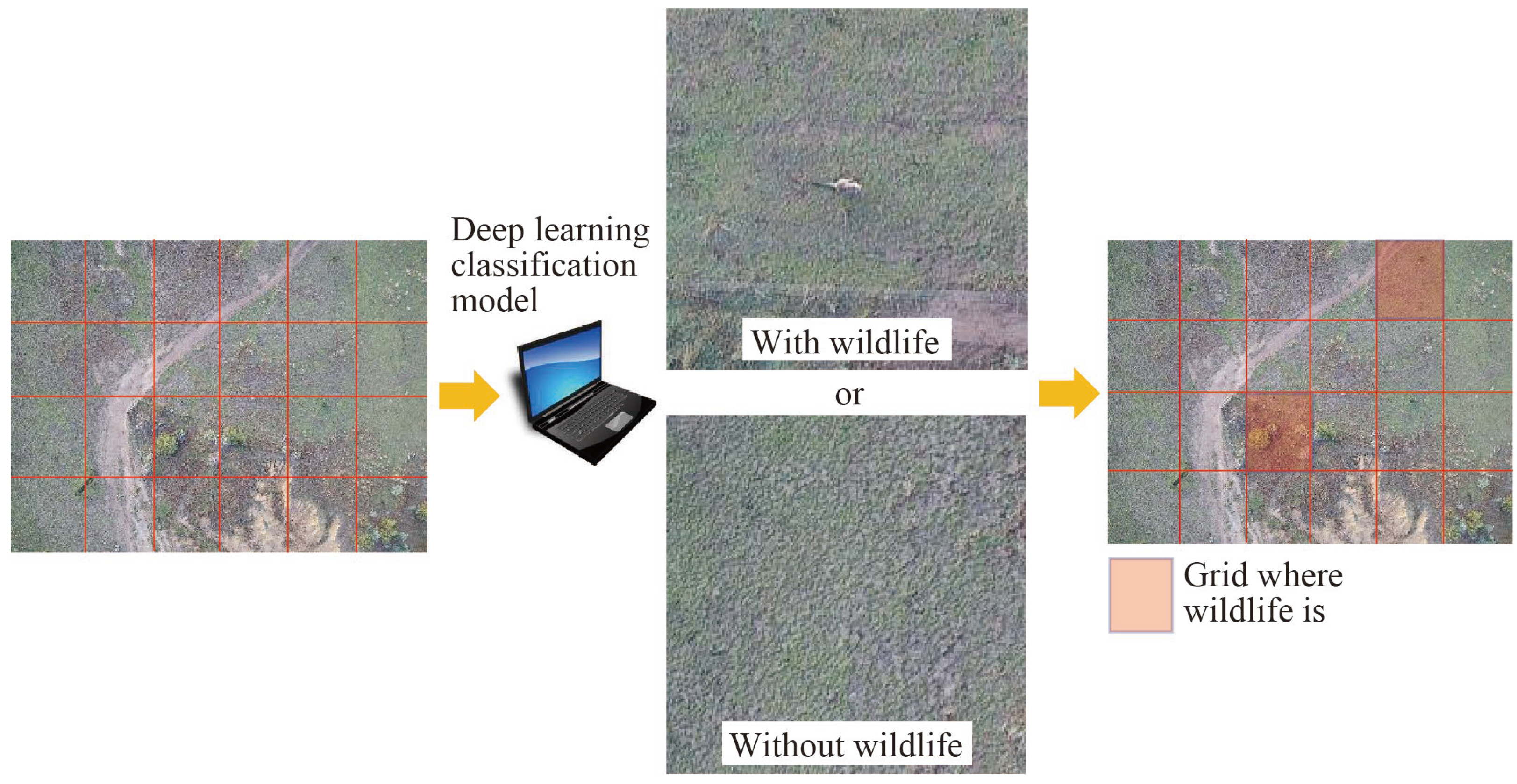
This section describes the two approaches for detecting moving wildlife in thermal images. To detect target objects, deep learning object detection models are generally used (hereinafter referred to as “detection methods”). Alternatively, by dividing input images into grids and classifying them as “with wildlife” or “without wildlife” with deep learning classification models, the grids where wildlife occurs can also be identified (hereinafter referred to as the “classification method” in Figure 2). In the second method, wildlife cannot be automatically counted because there are cases of wildlife in the grid image. However, the detection accuracy of the second method is generally higher than that of the first method because object detection models must simultaneously determine the target objects and their positions [21]. The results of the second method were used to preprocess the first method (Figure 3).
3.2. Color-Composite Image for a Pair of Thermal Images
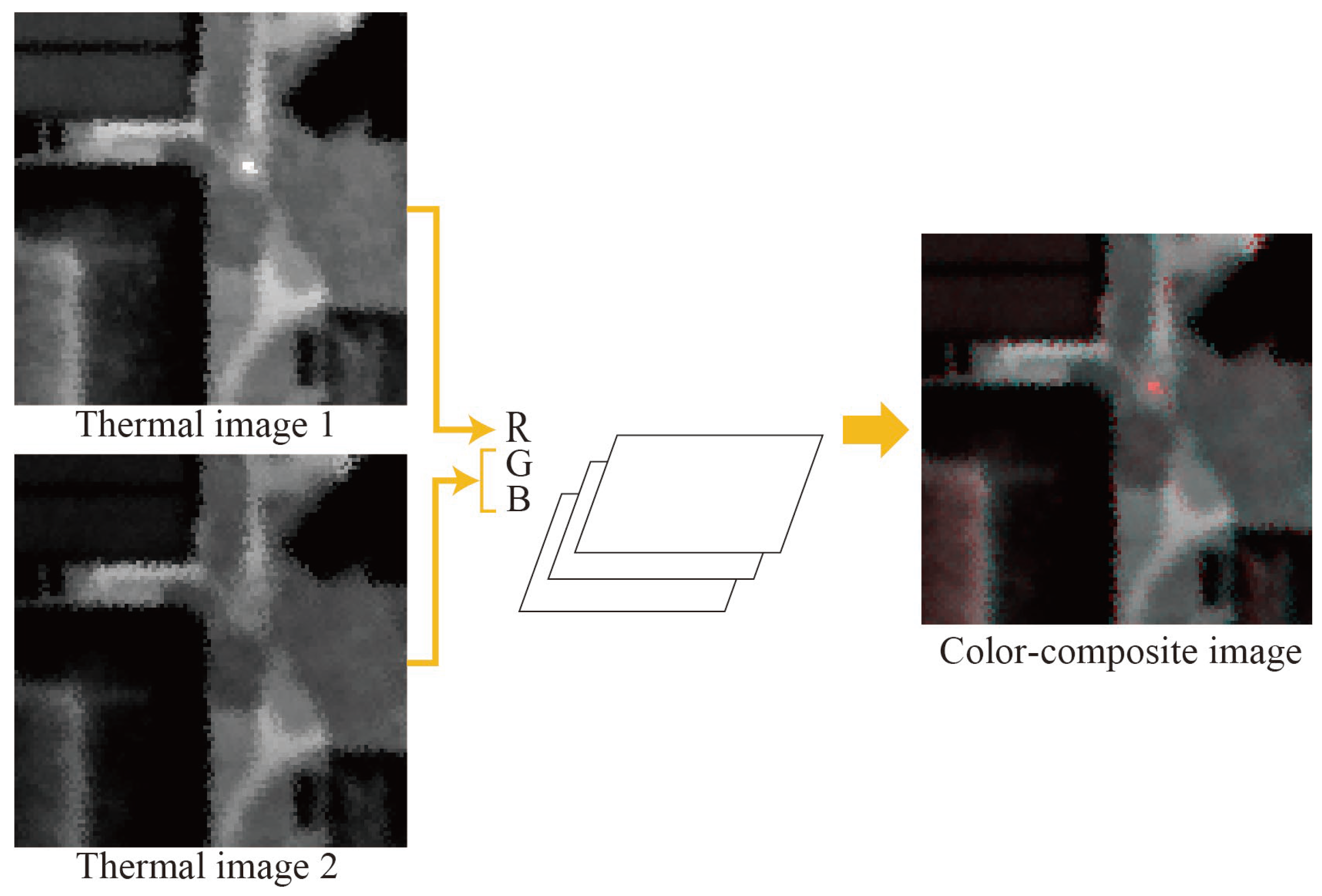
Visual inspection to create a training dataset is difficult because a large number of images must be checked. When using thermal images of an urban area because there are many hotspots, it is necessary to compare thermal infrared with time differences to detect moving wildlife, making visual inspection even more difficult. Therefore, we color-composited by assigning one thermal image to R and another to G and B (Figure 4). A moving hotspot is displayed in red or cyan to facilitate visual inspection. Color-composite images were used as input images for deep learning models to detect wildlife movement.
The 32-bit image format of the color-composite images was changed to an 8-bit image format in the surface temperature range of 15.0–20.0 °C, based on a previous study that showed that the surface temperature range of sika deer in the airborne thermal images was 17.0–18.0 °C [22]. Subsequently, the images were divided into grids, and annotations were added to the grid-divided images (Figure 5).
4. Results
4.1. Classification Method Results for Airborne Thermal Image
Three examinations were performed, as follows:
- Detection using a single thermal image.
Because wildlife is covered with fur, the difference between the surface and air temperatures is not very large. Furthermore, in thermal images, many objects, such as streetlights, appear as hot spots. Therefore, creating a training dataset from a single thermal image is difficult. However, a training dataset of single thermal images could be created by visually inspecting pairs of thermal images.
- 2.
- Standardization of the pairs of thermal images.
The shooting intervals caused a thermal gap between the two images due to radiative cooling. To reduce the impact of the thermal gap, deep learning classification models were trained and tested using standardized images such that the average and standard deviation between the paired images were the same.
- 3.
- Impact of different image sizes.
Visual inspection for creating training data cannot determine whether a hot spot is a moving object or local noise unless the image is of a certain size (over 100 × 100 pixels). Conversely, an image that is too large causes difficulty in detecting objects smaller than the input image size because there are few features of the objects themselves. When the convolution operation is repeated, the features of the objects and background are mixed, and the features of the background dominate those of the objects. Because the pixel resolution of airborne thermal images is 40 cm and the head and body lengths of sika deer are 90–190 cm [5], the area of sika deer ranges from 2 × 1 to 5 × 1 pixels. Therefore, we resized the images to 100 × 100 pixels using bilinear interpolation and changed the number of neurons in the input layer. The default number of neurons in the input layer is 224 × 224 × the number of channels (hereafter just written as “224 neurons”). Because an NVIDIA GeForce RTX 2080i with a video random access memory (VRAM) of 11 GB was used, the maximum number of neurons was limited by the VRAM capacity. Furthermore, we attempted to obtain an input image size of 224 × 224 pixels, which was larger than 100 × 100 pixels (Figure 6).
4.1.1. Classification Method Results Using Single Thermal Images
A dataset containing 232 “with deer” images and 239 “without deer” images was created. Then, “with deer” and “without deer” images were split into training (172, 179), validation (30, 30), and test (30, 30). Moreover, from other flight route images (FR2), a dataset of 277 “with deer” and 1600 “without deer”, which contained 206 “with car” and 1394 “other”, was also created for testing. It was difficult to distinguish cars from moving wildlife because cars are also moving hotspots; therefore, moving cars were separated in the latter dataset. Table 1 shows their classification accuracies with VGG-19 [23], DenseNet-121 [24], DenseNet-161 [24], Regnet_Y_32GF [25], EfficientNet_b0 [26], and a Vision Transformer (ViT) [27] using the PyTorch Torchvision models for classification.
No significant differences were observed in the classification accuracies of the five models. The classification accuracy of “car” was greater than that of “other”. Misclassified images of “other” contained hot spots such as a streetlight (Figure 7).
4.1.2. Classification Method Results Using a Standardized Thermal Image
The standardized image (Img_std) was calculated as follows:
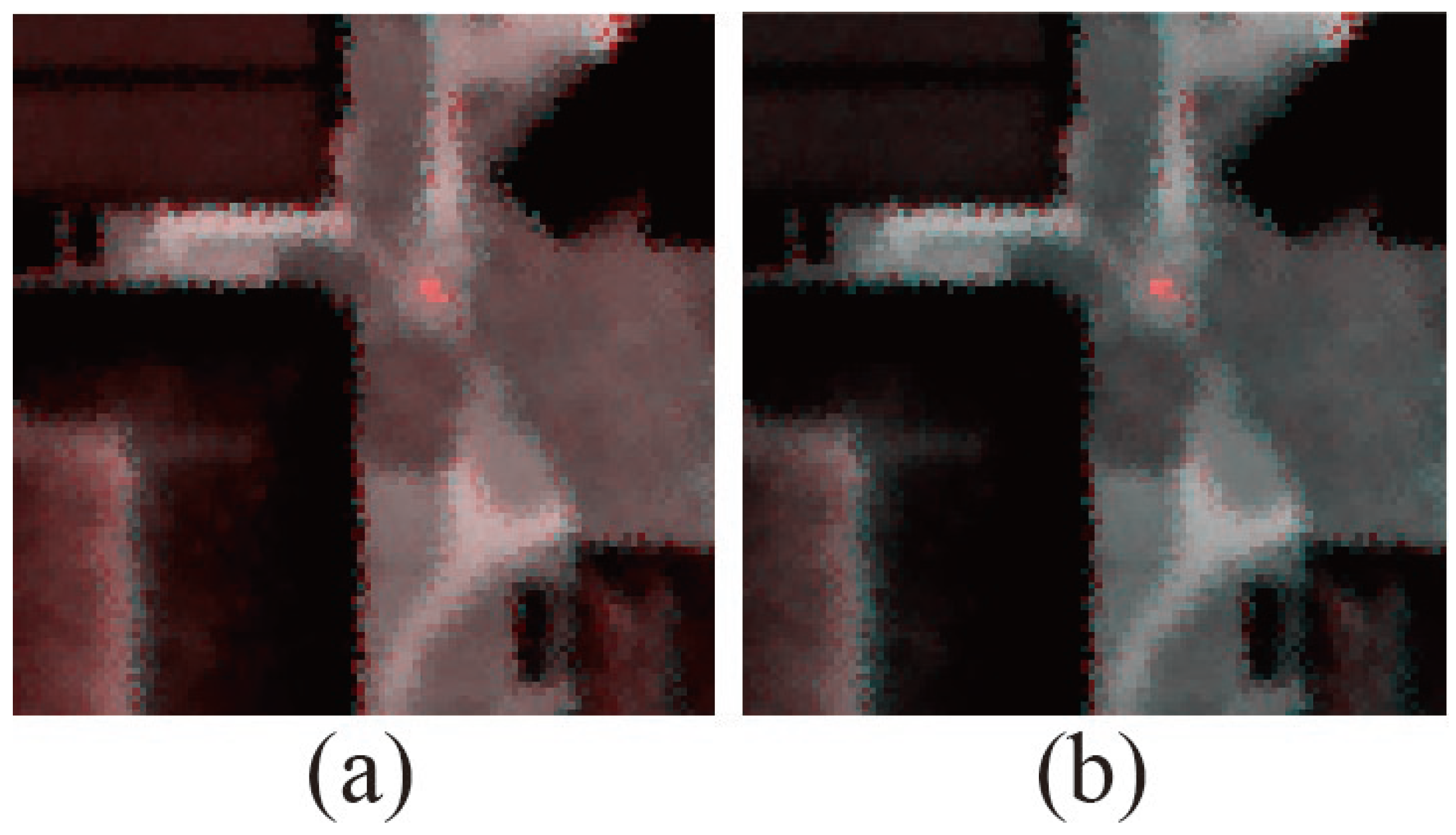
where Img1 and Img2 denote the pair of thermal images; Ave() and Stdev() denote the average and standard deviation operators, respectively; and (x, y) denote the coordinates. Figure 8 shows color-composite images with and without standardization.
Without standardization, there would be a temperature gap in the background owing to radial cooling caused by the difference in the shooting time of the paired images (Figure 8a). However, standardization eliminates the temperature gap in the background, making visual inspection easier (Figure 8b). A dataset containing 239 “with deer” and 240 “without deer” images in 100 × 100 pixels was created. Next, “with deer” and “without deer” images were split into training (179, 180), validation (30, 30), and test (30, 30). From other flight route images (FR2), a dataset of 299 “with deer” and 1600 “without deer”, which contained 206 “with car” and 1394 “other,” was also created for testing. Table 2 lists the classification accuracy obtained using standardized color composite images with 224 neurons in the input layer.
The classification accuracy of “car” was greater than that of “other”. The best averaged accuracy of “with deer” and “without deer” on FR2 was obtained with RegNet.
4.1.3. Classification Method Results with Different Image Sizes
A dataset was created using the same number of color-composite training images as that in Section 4.1.1 in 100 × 100 pixels; another dataset was created containing 252 “with deer” and 260 “without deer” images. Then, “with deer” and “without deer” images were split into training (192, 200), validation (30, 30), and test (30, 30) in 224 × 224 pixels.
Figure 9 shows the classification accuracies of VGG-19 based on the difference in the number of neurons in the input layer using images with 100 × 100 pixels in FR1.
The number of neurons had an insignificant effect on the classification accuracy of the “without deer” class. When the number was <200 or >500, the classification accuracy of the “with deer” class decreased. The best classification accuracy for “with deer” was 93% (without deer, 95%) with 300 and 400 neurons in the input layer. Table 3 lists the classification accuracies using color-composite images of 224 × 224 pixels, and Table 4 lists those of 100 × 100 pixels with 224 neurons in the input layer.
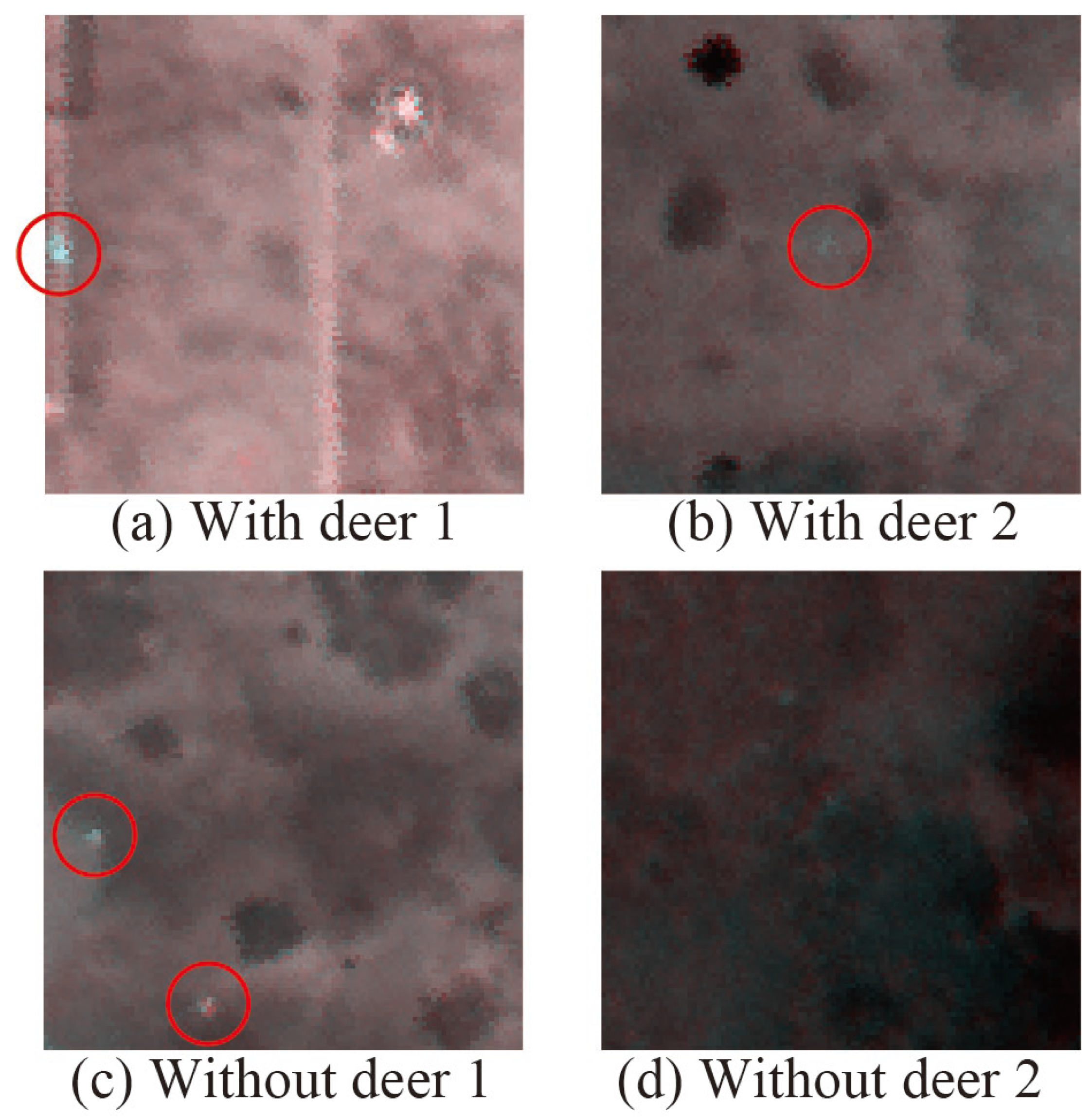
The classification accuracy obtained using 100 × 100-pixel images was better than that obtained using 224 × 224-pixel images. The classification accuracy of “car” was greater than that of “other”. The averaged accuracies of “with deer” and “without deer” on FR2 with DenseNet-121, DenseNet-161, and RegNet were better than those with VGG-19 and EfficientNet. Figure 10 shows the misclassified samples. To overlook the deer, there were some cases in which the deer was at the edge of an image (Figure 10a), and the gap in the surface temperature from the background was small (Figure 10b). To overestimate the number of deer, there were some cases of streetlights in a pair of images in which image registration was not good (Figure 10c) and in forest areas where image registration was not good (Figure 10d).
4.2. Detection Method Results for Airborne Thermal Images
A 100 × 100 pixel dataset containing 236 images from FR1 (607 deer) and 276 images from FR2 (915 deer) was created. The 236 images were divided into training (156), validation (30), and testing (50). A total of 276 images from FR2 were used for the testing. The proposed detection method was applied using the Faster R-CNN [28] and YOLOv8. YOLOv8 was introduced by Ultralytics in January 2023 [29] and there are five models: YOLOv8n, YOLOv8s, YOLOv8m, YOLOv8l, and YOLOv8x. YOLOv8n and YOLOv8x are the smallest and largest models, respectively. Because of the limitations of the VRAM capacity, YOLOv8n was used. The number of neurons in the input layer was 1500 for Faster R-CNN and 800 for YOLOv8.
4.2.1. Object Detection Method Results Using Standardized Thermal Images
The dataset was transformed into standardized color-composite images using Equation (1) to evaluate the effect of using standardized images on the proposed detection method. Table 5 shows the average precisions (APs) using standardized color composite images with the Faster R-CNN and YOLOv8. Three indices were used to evaluate the detection results: recall, precision, and AP. AP was defined as the area under the precision–recall (PR) curve. These indices were defined as follows:
where r and p denote the recall and precision, respectively, of the PR curve.
The APs of YOLOv8 were better than those of Faster R-CNN.
4.2.2. Object Detection Method Results with Different Image Sizes
Figure 11 and Figure 12 show the APs with the Faster R-CNN and YOLOv8, respectively, depending on the difference in the number of neurons in the input layer, using 100 × 100-pixel images.
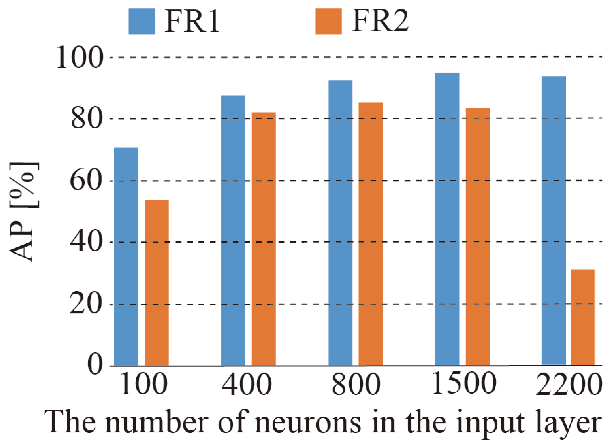
Because the VRAM capacity of the NVIDIA GeForce RTX 2080i was insufficient to process 2200 neurons in the input layer for YOLOv8, the NVIDIA Tesla V100, whose VRAM was 32 GB, was used. For the Faster R-CNN, using 1500 neurons in the input layer was the best for both APs on FR1 and FR2 at 92.3% and 85.8%, respectively (Figure 11). For YOLOv8, using 1500 neurons in the input layer was the best for AP on FR1 (94.7%); however, using 800 neurons was the best for AP on FR2 (85.3%; Figure 12).
Table 6 shows the classification accuracies using color-composite images of 224 × 224 pixels, and Table 7 shows those of 100 × 100 pixels with 1500 neurons in the input layer for the Faster R-CNN and 800 neurons in the input layer for YOLOv8.
The APs using 100 × 100-pixel images were better than those using 224 × 224-pixel images. In the cases using images with 100 × 100 pixels, there was no difference between Faster R-CNN and YOLOv8. Figure 13 shows the PR curves obtained using 100 × 100-pixel images.
The shape of the PR curve using the images of FR1 with Faster R-CNN was determined; recall and precision were 90.8% and 89.3%, respectively (red circles in Figure 13a). The shape of the PR curve using images of FR2 with Faster R-CNN was observed, and the recall and precision were 85.9% and 86.5%, respectively (red circles in Figure 13c). Figure 14 shows samples of the detection results. The labels were annotated using visual inspection as the ground truth (Figure 14a,c).
Comparing Figure 14a,b, there were two overestimations in the red and yellow circles. However, the detected object in the yellow circle might be a deer because it was overlooked during the visual inspection of the label image. Both the overestimations in the red circles (Figure 14b,d) were caused by image registration.
5. Discussion
Regarding the proposed classification method, because a car is a moving hot spot, we expected that it would be difficult to distinguish from moving wildlife; however, in the results, the classification accuracy of “car” was better than that of “other.” This may be because cars are larger than wildlife, which makes it relatively easy to distinguish between them. Comparing Table 1 and Table 4, the classification accuracy of “without deer” using single thermal images was lower than that using color-composite images of pairs of thermal images. The cause is nonmoving hot spots such as streetlights (Figure 7). These results indicate that even if training data were created, it would be difficult to classify wildlife and non-moving hotspots using single thermal images. A comparison of Table 2 and Table 4 indicates that the classification accuracies were not markedly different. Although standardization makes it easier to visually inspect images, it has little impact on the classification accuracy of deep-learning models. The models probably learned to ignore the differences in the background temperature. Therefore, although standardization cannot contribute to increasing accuracy, it can support visual interpretation when creating a training dataset.
At this time, the detection targets were extremely small (2–5 pixels). Therefore, this was a relatively difficult task. Therefore, two methods were investigated to increase the number of detection target pixels: enlarging the image bilinearly, increasing the number of neurons in the input layer, and increasing the size of the detection target relative to the image size by decreasing the grid division size of the image. The increase in classification accuracy for the “with deer” when the number of neurons was 100 to 200 (Figure 9) was thought to be due to this effect. Conversely, the decrease in classification accuracy for the “with deer” when the number of neurons was 500 to 700 was presumed to be due to the edges of the deer region becoming smoother due to bilinear image enlargement. In other words, the optimal number of neurons in the input layer is 200–500. This study used a bilinear method; however, the results may change if other methods are used. Therefore, investigating the optimal method is a future challenge. Comparing Table 3 and Table 4, the classification accuracies using color-composite images with 100 × 100 pixels were clearly greater than those using color-composite images with 224 × 224 pixels. When creating training data, humans check the movement of hot spots and their positions relative to the background and surrounding hot spots; therefore, if the image size is smaller than 100 × 100 pixels, it will not be possible to create the training dataset itself. Based on these results, by optimizing the number of neurons in the input layer, dividing the image into grids, and making the grid size as small as possible to create the training data, the classification accuracy can be improved by classifying images containing small objects.
In the case where there was a deer at the edge of the image (Figure 10a), “with deer” was not classified well. However, this can be solved using a moving window instead of grid division. Figure 10b shows the case where the difference between the surface temperature of the deer and the background temperature was small, and “with deer” was not classified well. This can be solved by shooting before sunrise or after sunset, when the gap between the surface and background temperatures increases. Another advantage of shooting during these times is that crepuscular wildlife is more active before sunrise or after sunset, making it easier to capture moving wildlife. However, the failure of classification with “without deer” was due to the failure of image registration. This study used images captured at flight altitudes of 1000 and 1300 m. By making the flight altitudes the same, Figure 10c can be solved. In addition, the eastern side of the shooting location was a hilly area, and the forest area was on a slope; therefore, image registration using a more accurate digital surface model with a structure for motion or aircraft light detection and ranging data can also be solved (Figure 10d).
For the proposed detection method, there was no statistical difference in the AP between Faster R-CNN and YOLOv8. Comparing Table 5 and Table 7, there was no difference between the standardized and non-standardized images. This result was the same as that of the proposed classification method. Comparing Table 6 and Table 7, the APs using color-composite images with 100 × 100 pixels were clearly greater than those using color-composite images with 224 × 224 pixels. This result was the same as that of the proposed classification method. The APs with YOLOv8n and 400 neurons in the input layers of FR1 and FR2 were 87.5% and 82.0%, respectively (Figure 12). In contrast, those with YOLOv8x were 85.5% and 76.2%, respectively. No statistical differences were observed between the two groups. In the case of YOLOv8x, it was not possible to increase the number of neurons in the input layer beyond 400 because of VRAM capacity limitations. In such cases, selecting a smaller model and increasing the number of neurons in the input layer can increase AP.
When putting the proposed methods into practical use, it is necessary to proceed with the development while considering the factors that have been clarified in previous research [8] in addition to the above findings, and a common improvement method should be employed when using deep learning models, such as increasing the training data for various cases. Previous research has indicated the importance of the factors listed below. The factors that determine the extraction of moving wildlife from remote sensing images have been discussed previously [8,9] as follows:
- To automatically extract targets from remote sensing images, the spatial resolution must be finer than one-fifth the body length of the target species. This yields two or more pure pixels that are not mixed with anything else. The head and body lengths of deer are 90–190 cm, and a spatial resolution of <20 cm is ideal. To achieve this spatial resolution, it is ideal to shoot at an altitude of ≤500 m [9]; however, there is a restriction on the minimum flight altitude. Therefore, high-resolution thermal image sensors or fixed-wing drones that do not generate propeller noise are used. Furthermore, fixed-wing drones can capture images more frequently than airborne drones, and by flying several fixed-wing drones simultaneously, it is possible to capture images efficiently with time differences. However, fixed-wing drones resemble large birds; therefore, even if they do not make a sound, there are concerns that the deer may become alarmed and stop moving. Therefore, when fixed-wing drones are used, it is necessary to evaluate their effects on deer in advance. It is believed that more accurate detection is possible by obtaining higher-resolution images using these methods.
- Objects under tree crowns did not appear in the aerial images. The possibility of extracting moving wildlife decreased as the area of the tree crowns in the image increased. Although a correction for the number of extracted moving wildlife using the proportion of forest is necessary for population estimates, it is not necessary to grasp population changes using the number of extracted wildlife as a population index [8,9].
- Wildlife exhibits well-defined activity patterns, such as sleeping, foraging, migration, feeding, and resting. To identify moving wildlife, the target species must move when conducting a survey. When the shooting intervals are too short, the targets cannot be extracted because the movement distance in a given interval must be longer than the body length. Shooting intervals were determined after surveying the movement speed of the target species during the observation period. Because the maximum walking speed of deer is 4 km/h [30] and the head and body lengths of sika deer are 90–190 cm, a shooting time difference of 2 s or more is required during deer movement. Because deer are crepuscular animals, it is better to shoot target areas multiple times in the early morning or evening, as in the present study [9]. Moreover, radiative cooling must be considered when determining shooting intervals. The surface temperature of wildlife covered with hair differs from the air temperature because the hair insulates the external heat. Although the gap in the surface temperature between the wildlife and background temperature was not large, the shooting intervals caused a thermal gap between the two images owing to radiative cooling. Therefore, shooting in the early morning is optimal [9]. The weather should also be considered for the same reason. Direct sunlight and shadows can affect surface temperature patterns, and direct sunlight reflection increases the surface temperature. Therefore, it is recommended that thermal images be captured on cloudy days. This study used images that were captured twice. However, because RGB images have three channels, the proposed method can be applied to three shots without changing the method. The proposed method cannot detect non-moving animals using a pair of images. However, by capturing two images with a relatively short time difference and then capturing another image after a certain time difference, it is possible to grasp behavioral patterns such as foraging or moving.
The classification test accuracies of “with deer” and “without deer” were >85% and >95%, respectively. The APs for detection, precision, and recall were >85%. Therefore, as explained in Section 3.1, the detection accuracies of the classification models were higher than those of the detection models. Furthermore, using a classification model with a method that can output activation maps, such as Grad-CAM [31], it is possible to show which objects in the image are wildlife. Users need to use detection models if they want to automatically count detected wildlife. Therefore, users can select the method depending on their purpose. As mentioned in Section 3, the proposed classification and detection methods can be combined. For example, if Faster R-CNN is used to process only the grids classified as “with deer” by VGG-19, multiplying the classification accuracy of “with deer” with VGG-19 by the recall of Faster R-CNN will approximately match the recall of the combination method. The calculation was 74.4% and 75.2% when the above process was performed. Over-detection can be reduced substantially because the classification accuracy of “without deer” and the average of “car” and “other” was 91.2%. Therefore, it is possible to use the proposed classification method when monitoring habitats, the proposed detection method when accurately counting the number of deer, or a combination of the classification and detection methods when monitoring increases or decreases rather than the number of individuals themselves, depending on the user’s objectives.
The proposed methods are more applicable to larger, moving wildlife and objects than to deer. However, when deer and wildlife of similar size are captured together in an image, it is difficult to distinguish them. If species identification is required in areas inhabited by wildlife of similar size—for instance, if the target animals are active during the daytime—the use of visible imagery should be considered. If the target animals are small animals, airborne thermal imagery will not provide sufficient resolution unless technological innovations, such as sensors, exist. In this case, the use of drones should be considered after considering their impact on the target species. In this study, the cars were not affected. This is presumably due to the difference in size between deer and cars, as well as the fact that the car body had cooled to about 13 °C by the shooting time. In the case of motorcycles, which are similar in size to deer, we considered that they were not affected because their engines and mufflers were considerably hotter. In some cases, road-masking processes may remove them.
In this study, the effectiveness of the proposed methods was demonstrated, and we will apply the proposed methods to other areas under various conditions to verify the generalization performance and work toward practical applications.
6. Conclusions
In this study, two methods—classification and object detection—were proposed to extract moving wildlife using pairs of airborne thermal images and deep learning models. The proposed methods were then applied to pairs of airborne thermal images. The classification test accuracies of “with deer” and “without deer” were >85% and >95%, respectively. The APs for detection, precision, and recall were >85%. This indicates that the proposed methods are practically accurate for monitoring changes in wildlife populations and can reduce the person-hours required to monitor a large number of thermal remote-sensing images. Furthermore, solutions were proposed for classifying and detecting failures. We implemented the proposed methods by clarifying the solutions and considering the factors identified in our previous research.
Author Contributions
Y.O. and H.O. conceived and designed the study; Y.O., N.Y. and H.O. performed the applicable evaluation; N.Y. performed preprocessing, including geometric correction of airborne images; Y.O. performed the evaluations, analyzed the results, and wrote the paper. All authors have read and agreed to the published version of the manuscript.
Funding
This study did not receive any specific grants from funding agencies in the public, commercial, or non-profit sectors.
Data Availability Statement
Data are contained within the article.
Acknowledgments
The authors thank Ryotaro Okamoto, University of Tsukuba, and Ryo Sugiura, NARO, for the useful discussions.
Conflicts of Interest
Author Natsuki Yoshida was employed by the company Nakanihon Air Co., Ltd. The remaining authors declare that the research was conducted in the absence of any commercial or financial relationships that could be construed as a potential conflict of interest. The authors declare no conflicts of interest. The founding sponsor had no role in the design of the study, collection, analysis, or interpretation of data, the writing of the manuscript, or the decision to publish the results.
References
- Schell, J.C.; Stanton, A.L.; Young, K.J.; Angeloni, M.L.; Lambert, E.J.; Breck, W.S.; Murray, H.M. The evolutionary consequences of human-wildlife conflict in cities. Evol. Appl. 2020, 14, 178–197. [Google Scholar] [CrossRef] [PubMed]
- Ravenelle, J.; Nyhus, J.P. Global patterns and trends in human-wildlife conflict compensation. Conserv. Biol. 2017, 31, 1247–1256. [Google Scholar] [CrossRef] [PubMed]
- Ministry of Agriculture, Forestry and Fisheries (MAFF). The 96th Statistical Yearbook of Ministry of Agriculture, Forestry and Fisheries. Available online: https://www.maff.go.jp/e/data/stat/96th/index.html (accessed on 13 March 2024).
- U.S. Department of the Interior. Adaptive Management. Available online: https://www.doi.gov/sites/doi.gov/files/uploads/TechGuide-WebOptimized-2.pdf (accessed on 13 March 2024).
- Ohdachi, S.D.; Ishibashi, Y.; Iwasa, M.A.; Saito, T. The Wild Mammals of Japan; Shoukadoh Book Sellers: Kyoto, Japan, 2009; ISBN 9784879746269. [Google Scholar]
- Oishi, Y.; Matsunaga, T.; Nakasugi, O. Automatic detection of the tracks of wild animals in the snow in airborne remote sensing images and its use. J. Remote Sens. Soc. Jpn. 2010, 30, 19–30, (In Japanese with English Abstract). [Google Scholar] [CrossRef]
- Chabot, D.; Francis, M.C. Computer-automated bird detection and counts in high-resolution aerial images: A review. J. Field Ornithol. 2016, 87, 343–359. [Google Scholar] [CrossRef]
- Oishi, Y.; Matsunaga, T. Support system for surveying moving wild animals in the snow using aerial remote-sensing images. Int. J. Remote Sens. 2014, 35, 1374–1394. [Google Scholar] [CrossRef]
- Oishi, Y.; Oguma, H.; Tamura, A.; Nakamura, R.; Matsunaga, T. Animal detection using thermal images and its required observation conditions. Remote Sens. 2018, 10, 1050. [Google Scholar] [CrossRef]
- Povlsen, P.; Linder, C.A.; Larsen, L.H.; Durdevic, P.; Arroyo, O.D.; Bruhn, D.; Pertoldi, C.; Pagh, S. Using drones with thermal imaging to estimate population counts of European hare (Lepus europaeus) in Denmark. Drones 2023, 7, 5. [Google Scholar] [CrossRef]
- Rancic, K.; Blagojevic, B.; Bezdan, A.; Ivosevic, B.; Tubic, B.; Vranesevic, M.; Pejak, B.; Crnojevic, V.; Marko, O. Animal detection and counting from UAV images using convolutional neural networks. Drones 2023, 7, 179. [Google Scholar] [CrossRef]
- Krishnan, S.B.; Jones, R.L.; Elmore, A.J.; Samiappan, S.; Evans, O.K.; Pfeiffer, B.M.; Blackwell, F.B.; Iglay, B.R. Fusion of visible and thermal images improves automated detection and classification of animals for drone surveys. Sci. Rep. 2023, 13, 10385. [Google Scholar] [CrossRef]
- Rebolo-Ifran, N.; Grilli, G.M.; Lambertucci, A.S. Drones as a threat to wildlife: YouTube complements science in providing evidence about their effect. Environ. Conserv. 2019, 46, 205–210. [Google Scholar] [CrossRef]
- Chretien, L.; Theau, J.; Menard, P. Visible and thermal infrared remote sensing for the detection of white-tailed deer using an unmanned aerial system. Wildl. Soc. Bull. 2016, 40, 181–191. [Google Scholar] [CrossRef]
- Kissell, R.E., Jr.; Tappe, P.A. Assessment of thermal infrared detection rates using white-tailed deer surrogates. J. Ark. Acad. Sci. 2004, 58, 70–73. [Google Scholar]
- Christiansen, P.; Steen, K.A.; Jorgensen, R.N.; Karstoft, H. Automated detection and recognition of wildlife using thermal cameras. Sensors 2014, 14, 13778–13793. [Google Scholar] [CrossRef] [PubMed]
- Terletzky, P.A.; Ramsey, R.D. Comparison of three techniques to identify and count individual animals in aerial imagery. J. Signal Inf. Process. 2016, 7, 123–135. [Google Scholar] [CrossRef]
- Ulhaq, A.; Adams, P.; Cox El, T.; Khan, A.; Low, T.; Paul, M. Automated detection of animals in low-resolution airborne thermal imagery. Remote Sens. 2021, 13, 3276. [Google Scholar] [CrossRef]
- Corcoran, E.; Winsen, M.; Sudholz, A.; Hamilton, G. Automated detection of wildlife using drones: Synthesis, opportunities, and constraints. Methods Ecol. Evol. 2021, 12, 1103–1114. [Google Scholar] [CrossRef]
- Geospatial Information Authority of Japan. Maps & Geospatial Information. Available online: http://www.gsi.go.jp/kiban/index.html (accessed on 13 March 2024).
- Suwa, K.; Cap, H.Q.; Kotani, R.; Uga, H.; Kagiwara, S.; Iyatomi, H. A comparable study: Intrinsic difficulties of practical plant diagnosis from wide-angle images. arXiv 2019, arXiv:1910.11506v2. [Google Scholar]
- Tamura, A.; Miyasaka, S.; Yoshida, N.; Unome, S. New approach of data acquisition using a state-of-the-art airborne sensor: Detection of wild animals using an airborne thermal sensor system. J. Adv. Surv. Technol. 2016, 108, 38–49. (In Japanese) [Google Scholar] [CrossRef]
- Simonyan, K.; Zisseman, A. Very deep convolutional networks for large-scale image recognition. arXiv 2014, arXiv:1409.1556. [Google Scholar]
- Huang, G.; Liu, Z.; Maaten, L.v.d.; Winberger, Q.K. Densely connected convolutional networks. arXiv 2017, arXiv:1608.06993. [Google Scholar]
- Xu, J.; Pan, Y.; Pan, X.; Hoi, S.; Yi, Z.; Xu, Z. RegNet: Self-regulated network for image classification. arXiv 2021, arXiv:2101.00590. [Google Scholar] [CrossRef] [PubMed]
- Tan, M.; Le, V.Q. EfficientNet: Rethinking model scaling for convolutional neural networks. arXiv 2019, arXiv:1905.11946. [Google Scholar]
- Dosovitskiy, A.; Beyer, L.; Kolesnikov, A.; Weissenborn, D.; Zhai, X.; Unterthiner, T.; Dehghani, M.; Minderer, M.; Heigold, G.; Gelly, S.; et al. An image is worth 16 × 16 words: Transformers for image recognition at scale. In Proceedings of the International Conference on Learning Representations (ICLR 2021), Vienna, Austria, 4 May 2021. [Google Scholar]
- Ren, S.; He, K.; Girshick, R.; Sun, J. Faster R-CNN: Towards real-time object detection with region proposal networks. In Proceedings of the Advances in Neural Information Processing Systems 28 (NIPS 2015), Montreal, QB, Canada, 7–12 December 2015. [Google Scholar]
- Ultralytics. YOLOv8. Available online: https://docs.ultralytics.com/ (accessed on 13 March 2024).
- Nelson, E.M.; Mech, L.D.; Frame, F.P. Tracking of white-tailed deer migration by global positioning system. J. Mammal. 2004, 85, 505–510. [Google Scholar] [CrossRef]
- Selvaraiu, R.R.; Cogswell, M.; Das, A.; Vadantam, R.; Parikh, D.; Batra, D. Grad-CAM: Visual explanations from deep networks via gradient-based localization. In Proceedings of the IEEE International Conference on Computer Vision, Venice, Italy, 22–29 October 2017; pp. 618–626. [Google Scholar] [CrossRef]
Figure 1.
Location of the airborne thermal image shooting area on a Sentinel2 image at Nara Park, Japan. Nara Park is located at the boundary between an urban region and a mountainous region. The base map was generated by the Geospatial Information Authority of Japan (https://maps.gsi.go.jp/development/ichiran.html, accessed on 13 March 2024).

Figure 2.
Wildlife detection using a deep learning classification model (classification method).

Figure 3.
Wildlife detection using a deep learning object detection model (detection method). Red rectangles indicate bounding boxes around detected wildlife.
Figure 3.
Wildlife detection using a deep learning object detection model (detection method). Red rectangles indicate bounding boxes around detected wildlife.

Figure 4.
Color-composite thermal image (100 by 100 pixels).

Figure 5.
Flow of the proposed methods to extract moving wildlife from pairs of thermal images.

Figure 6.
Two proposed approaches for extracting small objects. (a) Original. (b) The change in the number of neurons in the input layer. (c) The change in input image size.
Figure 6.
Two proposed approaches for extracting small objects. (a) Original. (b) The change in the number of neurons in the input layer. (c) The change in input image size.

Figure 7.
Misclassified cases of “other”.

Figure 8.
Color-composite images. (a) Without standardization. (b) With standardization.

Figure 9.
Classification accuracy with VGG-19 depending on the difference in the number of neurons in the input layer.
Figure 9.
Classification accuracy with VGG-19 depending on the difference in the number of neurons in the input layer.

Figure 10.
Misclassified samples. (a) There is a deer in a red circle at the edge of the image. (b) There is a deer in a red circle. (c) There are two streetlights in red circles. (d) In forest areas.
Figure 10.
Misclassified samples. (a) There is a deer in a red circle at the edge of the image. (b) There is a deer in a red circle. (c) There are two streetlights in red circles. (d) In forest areas.

Figure 11.
APs with Faster R-CNN depending on the difference in the number of neurons in the input layer.
Figure 11.
APs with Faster R-CNN depending on the difference in the number of neurons in the input layer.

Figure 12.
Average precision with YOLOv8 depending on the difference in the number of neurons in the input layer.
Figure 12.
Average precision with YOLOv8 depending on the difference in the number of neurons in the input layer.

Figure 13.
Precision–recall curves using color-composite images in 100 × 100 pixels. (a) Faster R-CNN using images on FR1. (b) YOLOv8 using images on FR1. (c) Faster R-CNN using images on FR2. (d) YOLOv8 using images on FR2.
Figure 13.
Precision–recall curves using color-composite images in 100 × 100 pixels. (a) Faster R-CNN using images on FR1. (b) YOLOv8 using images on FR1. (c) Faster R-CNN using images on FR2. (d) YOLOv8 using images on FR2.

Figure 14.
Samples of detection results. (a) Label on FR1. (b) Detection results on FR1. A detected object in a red circle was not deer; however, the other detected objects in the yellow circle might be deer. (c) Label on FR2. (d) Detection results on FR2. The detected object in the red circle is not a deer.


Table 1.
Classification accuracies using single thermal images.
| Flight Route | Class | VGG-19 | DenseNet-121 | DenseNet-161 | RegNet | EfficientNet | ViT | |
|---|---|---|---|---|---|---|---|---|
| FR1 | With deer | 80% | 90% | 87% | 93% | 80% | 90% | |
| Without deer | 83% | 87% | 93% | 90% | 90% | 83% | ||
| FR2 | With deer | 88.6% | 93.5% | 93.3% | 92.8% | 84.8% | 90.4% | |
| Without deer | Car | 86.1% | 82.0% | 81.6% | 92.4% | 82.6% | 90.7% | |
| Other | 74.3% | 68.4% | 73.8% | 68.1% | 74.2% | 79.1% |
Table 2.
Classification accuracies using standardized color-composite images.
| Flight Route | Class | VGG-19 | DenseNet-121 | DenseNet-161 | RegNet | EfficientNet | ViT | |
|---|---|---|---|---|---|---|---|---|
| FR1 | With deer | 90% | 90% | 97% | 90% | 87% | 90% | |
| Without deer | 93% | 93% | 97% | 97% | 97% | 90% | ||
| FR2 | With deer | 78.1% | 85.0% | 82.5% | 85.9% | 85.7% | 79.8% | |
| Without deer | Car | 98.0% | 97.2% | 93.1% | 99.2% | 96.9% | 99.0% | |
| Other | 92.0% | 78.0% | 87.5% | 90.5% | 77.8% | 81.9% |
Table 3.
Classification accuracies using color-composite images in 224 × 224 pixels.
| Flight Route | Class | VGG-19 | DenseNet-121 | DenseNet-161 | RegNet | EfficientNet | ViT |
|---|---|---|---|---|---|---|---|
| FR1 | With deer | 75% | 75% | 75% | 75% | 80% | 65% |
| Without deer | 80% | 75% | 75% | 75% | 70% | 50% |
Table 4.
Classification accuracies using color-composite images in 100 × 100 pixels.
| Flight Route | Class | VGG-19 | DenseNet-121 | DenseNet-161 | RegNet | EfficientNet | ViT | |
|---|---|---|---|---|---|---|---|---|
| FR1 | With deer | 90% | 93% | 90% | 90% | 90% | 93% | |
| Without deer | 97% | 97% | 100% | 100% | 100% | 93% | ||
| FR2 | With deer | 86.6% | 85.1% | 84.4% | 85.2% | 87.7% | 84.2% | |
| Without deer | Car | 96.5% | 99.3% | 99.1% | 98.8% | 91.1% | 97.3% | |
| Other | 85.9% | 95.9% | 95.1% | 94.4% | 88.9% | 90.9% |
Table 5.
Average precisions using standardized color-composite images.
| Flight Route | Faster R-CNN | YOLOv8 |
|---|---|---|
| FR1 | 90.1% | 92.6% |
| FR2 | 85.2% | 86.4% |
Table 6.
Average precisions using color-composite images in 224 × 224 pixels.
| Flight Route | Faster R-CNN | YOLOv8 |
|---|---|---|
| FR1 | 77.1% | 81.6% |
Table 7.
Average precisions using color-composite images in 100 × 100 pixels.
| Flight Route | Faster R-CNN | YOLOv8 |
|---|---|---|
| FR1 | 92.3% | 92.4% |
| FR2 | 85.8% | 85.3% |
Disclaimer/Publisher’s Note: The statements, opinions and data contained in all publications are solely those of the individual author(s) and contributor(s) and not of MDPI and/or the editor(s). MDPI and/or the editor(s) disclaim responsibility for any injury to people or property resulting from any ideas, methods, instructions or products referred to in the content. |
© 2024 by the authors. Licensee MDPI, Basel, Switzerland. This article is an open access article distributed under the terms and conditions of the Creative Commons Attribution (CC BY) license (https://creativecommons.org/licenses/by/4.0/).
Share and Cite
MDPI and ACS Style
Oishi, Y.; Yoshida, N.; Oguma, H. Detecting Moving Wildlife Using the Time Difference between Two Thermal Airborne Images. Remote Sens. 2024, 16, 1439. https://doi.org/10.3390/rs16081439
AMA Style
Oishi Y, Yoshida N, Oguma H. Detecting Moving Wildlife Using the Time Difference between Two Thermal Airborne Images. Remote Sensing. 2024; 16(8):1439. https://doi.org/10.3390/rs16081439
Chicago/Turabian StyleOishi, Yu, Natsuki Yoshida, and Hiroyuki Oguma. 2024. "Detecting Moving Wildlife Using the Time Difference between Two Thermal Airborne Images" Remote Sensing 16, no. 8: 1439. https://doi.org/10.3390/rs16081439
Note that from the first issue of 2016, this journal uses article numbers instead of page numbers. See further details here.