A Real-Time Method for Railway Track Detection and 3D Fitting Based on Camera and LiDAR Fusion Sensing

Abstract

Railway track detection, which is crucial for train operational safety, faces numerous challenges such as the curved track, obstacle occlusion, and vibrations during the train’s operation. Most existing methods for railway track detection use a camera or LiDAR. However, the vision-based approach lacks essential 3D environmental information about the train, while the LiDAR-based approach tends to detect tracks of insufficient length due to the inherent limitations of LiDAR. In this study, we propose a real-time method for railway track detection and 3D fitting based on camera and LiDAR fusion sensing. Semantic segmentation of the railway track in the image is performed, followed by inverse projection to obtain 3D information of the distant railway track. Then, 3D fitting is applied to the inverse projection of the railway track for track vectorization and LiDAR railway track point segmentation. The extrinsic parameters necessary for inverse projection are continuously optimized to ensure robustness against variations in extrinsic parameters during the train’s operation. Experimental results show that the proposed method achieves desirable accuracy for railway track detection and 3D fitting with acceptable computational efficiency, and outperforms existing approaches based on LiDAR, camera, and camera–LiDAR fusion. To the best of our knowledge, our approach represents the first successful attempt to fuse camera and LiDAR data for real-time railway track detection and 3D fitting.

1. Introduction

Safety is crucial for railway transportation [1,2,3]. Effective railway track detection ensures the accuracy of obstacle detection [4,5,6] and the security of the autonomous train. However, existing research studies mainly focus independently on either the semantic segmentation or the point cloud segmentation of tracks, with limited studies integrating the two to achieve distant railway track detection and vectorization.

1.1. Background

To reduce railway accidents, numerous research studies have been focused on automatic railway track detection [7,8,9]. Currently, two primary sensors are commonly employed in existing methods: the camera and LiDAR. Methods based on vision and those based on LiDAR each have distinct strengths and weaknesses in the railway track detection.

The images contain rich texture and color information, enabling accurate railway track semantic segmentation [10,11,12]. Using a high-resolution camera, more accurate information about distant railway tracks can be obtained. The semantic segmentation of the railway track can be mapped to the bird’s-eye view (BEV) using a transformation matrix, which in fact realizes the distant railway track detection with 3D information [13]. However, this method lacks 3D information about the surrounding environment, and its transformation matrix is fixed, leading to limited robustness against changes in extrinsic parameters. Additionally, the camera is susceptible to illumination variations, particularly in low-illumination conditions, which significantly impairs our perception of the surrounding environment.

LiDAR-based methods provide precise, accurate 3D information about the shape and position of the track [14,15], while also exhibiting robustness to changes in illumination. However, LiDAR-based methods detect shorter track lengths, constrained by the LiDAR performance and the low reflectivity of the track surface. Even with high-performance LiDAR, which is more expensive, the acquired railway point cloud becomes sparser as the distance increases, resulting in a significantly shorter detection range compared to high-resolution cameras. Additionally, after rainfall, a layer of water film forms on the surface of the railway, reducing its reflectivity and further limiting the detection distance of LiDAR. Without distant railway track point clouds, we cannot accurately determine the trajectory of the tracks. This poses safety risks to train operation.

In recent years, research on the fusion of camera and LiDAR data has gained increasing attention, gradually extending into the field of railway transportation [16,17]. Due to the complementarity of the camera and LiDAR, the fusion of the camera and LiDAR can achieve more accurate and distant railway track perception.

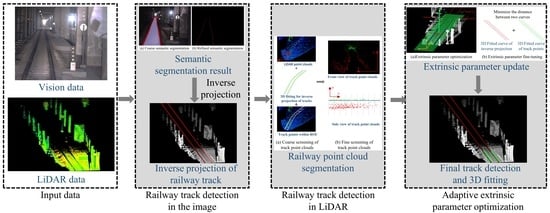
Accordingly, this paper proposes a real-time railway track detection and 3D fitting framework that integrates the camera and the LiDAR data. Figure 1 demonstrates the framework of the proposed method. Firstly, synchronized data captured by the onboard camera and LiDAR are acquired. Subsequently, the architecture is divided into three stages: railway track detection in the image, railway track detection in LiDAR, and adaptive extrinsic parameter optimization.

In the first stage, the semantic segmentation of railway tracks is performed. Subsequently, the inverse projection is applied to the semantic segmentation to obtain the 3D information of the tracks.

In the second stage, 3D fitting is applied to the inverse projection of the tracks for track vectorization and then is used to determine the region of interest (ROI) and obtain the LiDAR point clouds in the region. Subsequently, post processing is applied to obtain points representing the surface of the railway tracks.

In the third stage, LiDAR points and the inverse projection of railway tracks are used to optimize the extrinsic parameters between coordinate systems.

1.2. Contributions

The main contributions of this paper include the following:

(1)

A real-time railway track detection and 3D fitting framework based on camera and LiDAR fusion sensing is designed. The framework includes railway track detection in the image, railway track detection in LiDAR, and adaptive extrinsic parameter optimization. It exhibits robust performance in challenging scenarios such as a curved track, obstacle occlusion, and vibrations during the train’s operation.

(2)

An inverse projection and 3D fitting method for semantic segmentation of railway tracks is proposed. The 3D track vectorization and accurate environmental information establish a foundational basis for subsequent analysis and decision-making in autonomous train systems.

(3)

An accurate segmentation method for railway track point clouds is proposed. The method utilizes the inverse projection of railway tracks to segment the point clouds, achieving a significant improvement in accuracy compared to existing methods. It also demonstrates superior accuracy in distinguishing points like track bed points that are prone to being misclassified as track points during segmentation.

1.3. Paper Organization

The remainder of this paper is structured as follows. Section 2 gives a brief overview of related approaches that deal with railway track detection, followed by a detailed presentation of the railway track detection and 3D fitting approach in Section 3. Section 4 shows the experimental results. Finally, the conclusion is presented in Section 5.

2. Related Work

Currently, railway track detection [18] has gained widespread attention and become an important module of automated train systems. Generally, current methods of railway track detection fall into three categories: vision-based approaches, LiDAR-based approaches, and fusion-based approaches.

2.1. Vision-Based Approach

Traditional railway track segmentation methods are based on the computer vision features and geometric features of the railway track. Qi et al. [19] computed the histogram of oriented gradients (HOG) features of railway images, established integral images, and used a region-growing algorithm to extract the railway tracks. Nassu and Ukai [20] achieved railway extraction by matching edge features to candidate railway patterns which were modeled as sequences of parabola segments. Recently, with the development of deep learning and the publication of datasets for semantic scene understanding for autonomous trains and trams [21,22], methods based on deep learning have been widely used in railway track detection. Wang et al. [7] optimized the SegNet to achieve railway track segmentation by adding dilated cascade connections and cascade sampling. An improved polygon fitting method was applied to further optimize the railway track. Wang et al. [8] modified the ResNet [23] to extract multi-convolution features and used a pyramid structure to fuse the features. Yang et al. [13] proposed a topology-guided method for rail track detection by applying an inverse perspective transform to rail-lanes. These methods based on deep learning enhance the performance of the railway track segmentation and demonstrate robust adaptability to the shape of the track. However, it should be noted that those methods appear incapable of providing accurate 3D information about the railway track.

2.2. LiDAR-Based Approach

Compared to images, LiDAR provides accurate geospatial and intensity information. In addition, point clouds are robust to illumination variations. Traditional methods [15,24] classify point clouds according to the geometric and spatial information, thereby achieving the segmentation of railway tracks. Some studies [25,26] have used LiDAR density for the segmentation of railway infrastructure. Deep learning techniques have been widely used in railway transportation. PointNet and KPConv were combined by Soilán et al. [27] to obtain a similar performance to the heuristic algorithm in a railway point cloud segmentation study. Due to the limited railway data, the trained network is prone to overfitting, making it difficult to ensure the algorithm’s robustness in other scenes. Jiang et al. [28] proposed a framework named RailSeg, which contains integrated local–global feature extraction, spatial context aggregation, and semantic regularization. This method is computationally intensive and is difficult to be applied in real time. In addition, it tends to confuse railway track points with ground points, resulting in a relatively low precision in the segmentation of railway track point clouds. So far, there is limited research on the real-time segmentation of distant railway tracks using single-frame LiDAR data [14]. While some studies [25,28,29,30] claim high precision and recall in railway track point cloud segmentation, most of them are conducted on non-real-time processing using data collected from Mobile Laser Scanning (MLS). Moreover, these methods rely on the elevation of the point cloud for segmentation, which may fluctuate significantly due to the installation angle of the LiDAR sensor, terrain variations, and train vibrations, resulting in misclassification of track beds and rail tracks.

2.3. Fusion-Based Approach

Due to inherent limitations of each single sensor, multi-sensor fusion is increasingly becoming popular, and has been applied to autonomous vehicles. Wahde et al. [31] trained several fully convolutional neural networks for road detection by fusing LiDAR point clouds and camera images. Jun et al. [32] proposed a fusion framework, which contained a LiDAR-based weak classifier and a vision-based strong classifier, for pedestrian detection. So far, limited studies have been conducted on railway track detection by fusing camera and LiDAR data. Wang et al. [17] proposed a framework for railway object detection. A multi-scale prediction network is designed for railway track segmentation via the image. And the LiDAR points are mapped onto the image through coordinate projection [33] to obtain the LiDAR points within the railway track area. In practical application, the inherent limitations of LiDAR and the low reflectivity of the railway track surface pose challenges in obtaining railway track points at extended distances. Consequently, accurately determining the trajectory of the railway track in a 3D space becomes a formidable task. Inspired by these methods, this study aims to fuse vision and LiDAR data to achieve distant railway track detection with 3D information.

3. Approach

3.1. Railway Track Detection in the Image

In this study, the railway track detection and 3D fitting aims to obtain the spatial coordinates of the tracks to determine their accurate 3D trajectory. It should be noted that we do not intend to model the detailed size and external shape of the tracks [34,35]. Therefore, a two-stage method for railway track detection in the image is proposed.

In order to extract the railway track pixels from the image, we carry out the first stage of railway track detection in the image—semantic segmentation. Through this stage, the railway track pixels are extracted from the image.

The geometric properties of the railway tracks in the camera view are not obvious. So, we carry out the second stage of railway track detection in the image—inverse projection. Through this stage, the 3D coordinates of the railway tracks are obtained, allowing us to explore the geometric characteristics of the railway tracks.

3.1.1. Railway Track Semantic Segmentation

A semantic segmentation network is applied to obtain the accurate rail pixels in the image. We employ the on-board camera and LiDAR. To address the stability concerns during the train’s operation, we apply a classical lightweight semantic segmentation network, BiSeNet V2 [36], which ensures the computational efficiency and speed. The model is trained on a public dataset [21] for semantic scene understanding for trains and trams, employing three classification labels: rail-raised, rail-track, and background. The segmentation results of the model for the railway track are depicted in Figure 2b, where red pixels represent the railway tracks, and purple pixels represent the railway track area. From the output results, the semantic segmentation of the railway tracks is extracted, as shown in Figure 2c.

The semantic segmentation results appear coarse, directly transforming them through inverse projection into a 3D space would hinder the accurate extraction of the railway track trajectory. Therefore, we refine the semantic segmentation by obtaining the centerline of the railway track, which serves as the final representation of the railway track, as shown in Figure 2d.

3.1.2. Inverse Projection

With the semantic segmentation of the tracks, the inverse projection of the tracks can be performed. Figure 3 illustrates the positions of the camera and LiDAR on the train, along with the coordinate systems for the camera, LiDAR, and the rail.

To enhance the reflectivity of the railway track surface for obtaining points at a greater distance, the camera and LiDAR are tilted downward. All these coordinate systems adhere to the right-hand coordinate system convention of OpenGL. The transformation relationship between the coordinate systems is defined by Equation (1), where the points $P_l$, $P_c$, and $P_r$ are the coordinates of the same point $P$ in the LiDAR coordinate system, camera coordinate system, and rail coordinate system, respectively. $R_1$, $R_2$, and $R_3$ are rotation matrices, and $t_1$, $t_2$, and $t_3$ are translation matrices between the coordinate systems.

$$\left\{\begin{array}{c}{P}_l=R_1{P}_r+t_1\\ P_l=R_2{P}_c+t_2\\ P_c=R_3{P}_r+t_3\end{array}\right.$$

(1)

The transformation relationship between the camera coordinate system and the pixel coordinate system is represented by Equation (2), where $K^{-1}$ represents the inverse of the camera intrinsic parameter matrix $K$, which is obtained through camera calibration [37] before the train’s operation, and $Z_c$ is the depth from the object point to the image plane. Clearly, to obtain the 3D coordinates of railway tracks, it is essential to determine the depth $Z_c$ corresponding to each pixel on the tracks.

$$\left[\begin{array}{c}{X}_c\\ Y_c\\ Z_c\end{array}\right]=Z_c{K}^{-1}\left[\begin{array}{c}u\\ v\\ 1\end{array}\right], K=\left[\begin{array}{ccc}{f}_x& 0& u_0\\ 0& f_y& v_0\\ 0& 0& 1\end{array}\right]$$

(2)

Two assumptions are proposed based on the geometric characteristics of the railway tracks:

(1)

Within a short distance in front of the train, the slope of the railway tracks changes slowly [13].

(2)

In the semantic segmentation of railway tracks, points represented by the same $v$ maintain the same depth $Z_c$.

In assumption (1), we only consider a short distance ahead of the train (200 m), and the variation in slope within this range is negligible. Assessing whether the railway tracks within this range are on a plane should be based on the variation in slope rather than the slope itself. In assumption (2), at curve tracks, the heights of the inner and outer tracks vary, resulting in different v-values for points with the same depth $Z_c$. However, due to the large curvature radius of the railway tracks, during the inverse projection, the differences in v-values mainly manifest in longitudinal deviations, while lateral deviations are relatively smaller. Considering the continuity of the railway tracks, the impact of longitudinal deviations on train operation safety is much smaller than that of lateral deviations, making errors associated with assumption (2) acceptable in practical applications.

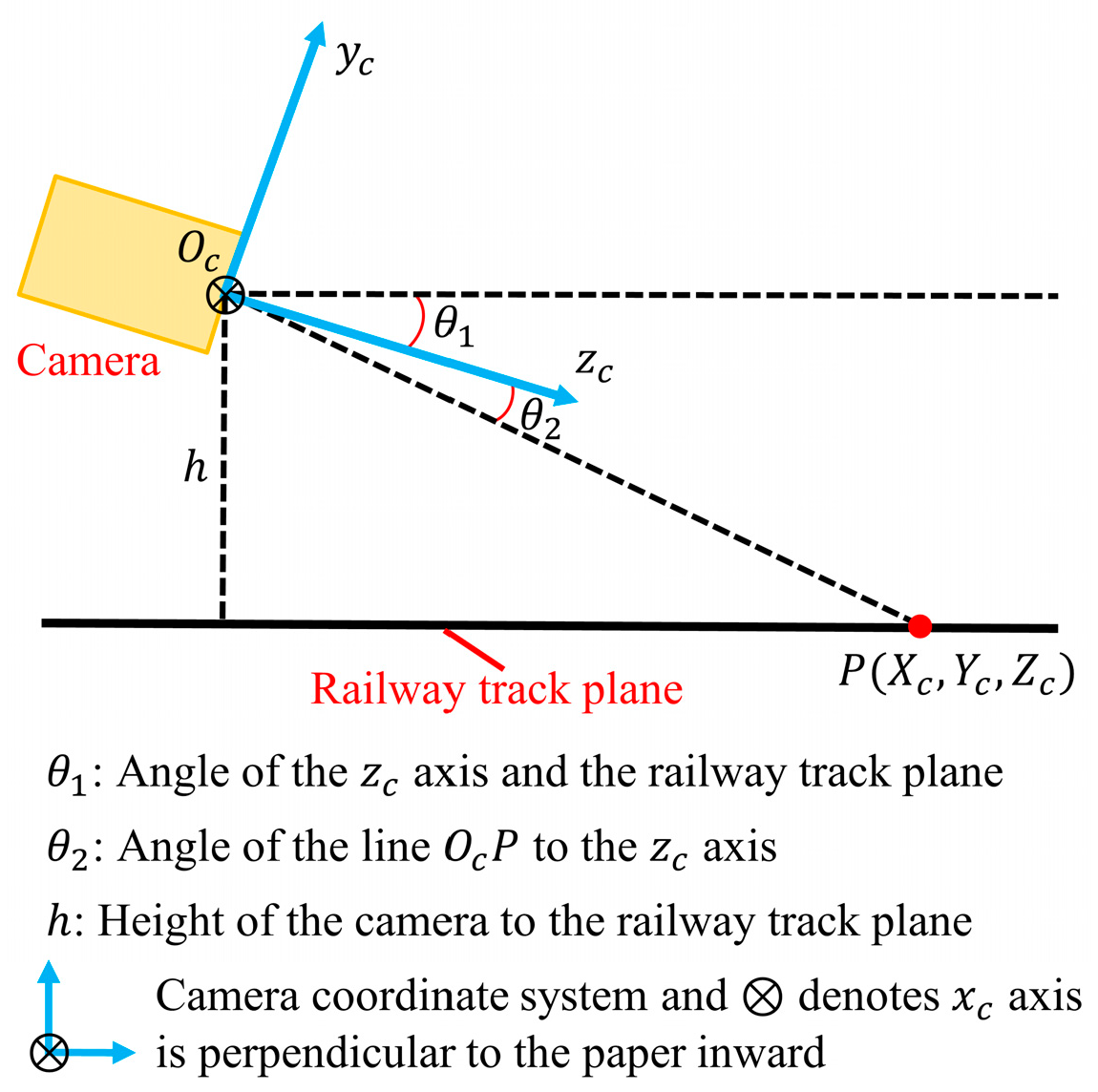
Figure 4 illustrates the side view of the camera. Once the camera is installed, the camera’s mounting height $h$ and the angle ${\theta }_1$ between the camera optical axis $z_c$ and the railway track plane are thereby determined. For any point $P$ on the surface of the railway track, the 3D coordinates of that point can be determined by knowing the angle ${\theta }_2$ of the line $O_{c}P$ to the $z_c$ axis, as shown in Equation (3), where $\left|O_{c}P\right|$ represents the length of the line segment $O_{c}P$.

$$Z_c=\left|O_{c}P\right|·cos{\theta }_2=\frac{h}{\sin \left({\theta }_1+{\theta }_2\right)}·cos{\theta }_2$$

(3)

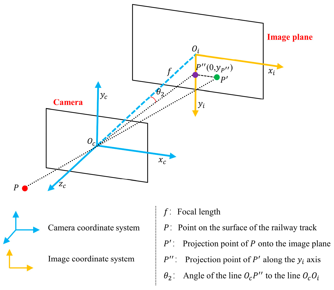
Figure 5 illustrates the pinhole camera model. Based on assumption (2), points projected onto the line $P^{\prime }{P}^{″}$ possess the consistent depth $Z_c$ in the camera coordinate system. The angle of the line $O_c{P}^{″}$ to the line $O_c{O}_i$ corresponds to ${\theta }_2$ as defined in Equation (3). Based on geometric relationships, ${\theta }_2$ can be computed by Equation (4), where $y_{P^{″}}$ is the y-coordinate of point $P^{″}$ in the image coordinate system, $f$ is the focal length, $v$ is the ordinate of the point $P^{″}$ in the pixel coordinate system, $v_0$ is the ordinate of the camera’s optical center in the coordinate system, $dy$ is the physical size of each pixel on the camera sensor, and $f_y$ is the focal length expressed in pixels. The values $v_0$ and $f_y$ can be obtained through camera calibration [37].

$${\theta }_2=arctan\frac{y_{P^{″}}}{f}=arctan\frac{\left(v-v_0\right)dy}{f}=arctan\frac{v-v_0}{f_y}$$

(4)

By integrating Equations (2)–(4), the camera coordinates of the railway track can be determined from its pixel coordinates, as expressed in Equation (5).

$$\left[\begin{array}{c}{X}_c\\ Y_c\\ Z_c\end{array}\right]=\frac{h}{\mathrm{s}\mathrm{i}\mathrm{n}({\theta }_1+arctan\frac{v-v_0}{f_y})}\cos \left(arctan\frac{v-v_0}{f_y}\right)K^{-1}\left[\begin{array}{c}u\\ v\\ 1\end{array}\right]$$

(5)

Based on Equation (1), the camera coordinates of the railway track points are transformed into LiDAR coordinates. The LiDAR and camera are rigidly mounted together, and the extrinsic parameters between them are theoretically constant, which can be determined through LiDAR–camera calibration [38] before the train operation.

3.2. Railway Track Detection in LiDAR

In this stage, 3D fitting is applied to the inverse projection for track vectorization. Subsequently, the 3D fitted curve is utilized to determine the ROI and filter the LiDAR track points within the ROI.

3.2.1. Application of 3D Fitting

The 3D fitting involves curve fitting of spatial points, using the piecewise functions to ensure robustness in both straight and curve track scenarios, as illustrated in Figure 6.

For each fixed length, such as 10 m, a segmented interval is established, with each subfunction maintaining the same function form but varying parameters. The form of each subfunction is illustrated in Equation (6), where $i$ presents the interval to which the point belongs. To ensure continuity and accuracy between adjacent intervals, when computing the subfunction for the current interval, points from both the current interval and its neighboring intervals are included in the curve fitting calculation.

$$\left\{\begin{array}{c}{x}_i=f_i(z_i)={\displaystyle \sum _{j=0}^2}{a}_j{z}_i^j\\ y_i=g_i(z_i)={\displaystyle \sum _{j=0}^1}{b}_j{z}_i^j\end{array}\right.$$

(6)

Additionally, the curvature of the railway track is small. Therefore, it is necessary to apply curvature constraints to the fitted track curve. For the polynomial curve $f\left(z\right)$, its curvature is defined as shown in Equation (7), where $a_2$ corresponds to the coefficient of the quadratic term in Equation (6). The curvature of the quadratic curve $f\left(z\right)$ is maximal at its extreme point. Constraining the curvature at that point leads to an optimization problem with constraints, as depicted in Equation (8), where n represents the number of LiDAR points and $R$ represents the minimum constraint radius we set.

$$k=\frac{{|f}^{″}\left(z\right)|}{{\left(1+{\left(f^{\prime }\left(z\right)\right)}^2\right)}^3}\le \left|2a_2\right|$$

(7)

$$\left\{\begin{array}{l}\left[a_0,a_1,a_2\right]=argmin {\displaystyle \sum _{i=1}^n}{\left(f\left(z_i\right)-x_i\right)}^2,subject to \left|2a_2\right|<\frac{1}{R}\\ \left[b_0,b_1\right]=argmin {\displaystyle \sum _{i=1}^n}{\left(g\left(z_i\right)-y_i\right)}^2\end{array}\right.$$

(8)

The parallel constraint is applied to the left and right tracks to ensure their respective fitting curves $f\left(z\right)$ have identical coefficients for both the quadratic and linear terms. This constraint implies that the left and right tracks only have translation differences along the x-axis. In other words, the left and right tracks share the same parameters $a_1$, $a_2$, and $b_2$, differing only in $a_0$ and $b_0$.

3.2.2. Railway Track Point Cloud Segmentation

The Railway track point cloud segmentation process is illustrated in Figure 7. Initially, the 3D fitted curve is utilized to determine the ROI and filter the LiDAR track points within the ROI, as illustrated in Figure 7a.

Post processing is applied to these LiDAR point clouds to extract the surface point clouds of the railway track. The details of the post processing are elaborated as follows:

(1)

Divide small intervals such as 1 m along the z-axis and select points with relatively higher y-values in each interval, as illustrated in Figure 7b.

(2)

Divide these points into two groups based on their z-values, such as points within 50 m and those beyond 50 m. Apply the Random Sample Consensus (RANSAC) algorithm [39] to perform plane fitting on the near track points and pick out the near track points on the fitted plane. Compute the distances from the distant track points to the fitted plane and select the distant track points that are relatively close to the fitted plane, as illustrated in Figure 7c.

(3)

Merge the two sets of selected near and distant track points. The differences between segmented railway track points and ground truth are shown in Figure 7d.

The presence of obstacles significantly increases the maximum height value of the point cloud, potentially causing track points not to be selected. Partitioning smaller intervals can effectively reduce the impact of obstacles. Employing the RANSAC algorithm for plane fitting can further remove the track bed points. Constrained by the performance of LiDAR, as the distance increases, the reliability of the point clouds decreases. Therefore, fitting the railway track plane using nearby track points achieves more accurate results. After employing such a post processing procedure, accurate point clouds of the railway track surface can be obtained.

3.3. Adaptive Extrinsic Parameter Optimization

The camera and LiDAR are fixed on a device, which is subsequently installed on the train. This setup ensures the constancy of the extrinsic parameters between the camera and LiDAR. During the actual operation of the train, slight vibrations may occur. Additionally, when the train ascends or descends slopes, the angle between the camera’s optical axis and the railway track plane may change. This indicates that the extrinsic parameters between the camera and the rail coordinate system may change. Applying inverse projection to the semantic segmentation of the railway track and transforming it to the LiDAR coordinate system with incorrect extrinsic parameters leads to deviations from reality. Therefore, the adaptive extrinsic parameter optimization becomes crucial.

In this study, the extrinsic parameters between the camera and LiDAR are assumed to be constant. If the adaptive optimization of the extrinsic parameters between the LiDAR and the rail coordinate systems is achieved, then based on Equation (1), the extrinsic parameters between the camera and the rail coordinate systems can be computed.

As illustrated in Figure 3, in the rail coordinate system the origin is located at the center of the left and right railway tracks below the LiDAR. The x-axis is oriented perpendicular to the right railway track, pointing towards the left railway track. The y-axis is vertical to the railway track plane pointing upwards. The z-axis aligns with the forward direction of the train’s head, specifically following the tangent direction of the railway track. Using the LiDAR point clouds of the left and right railway tracks, the position of the rail coordinate system in the LiDAR coordinate system can be determined. Subsequently, the extrinsic parameters between the LiDAR coordinate system and the rail coordinate system can be calculated.

The three axes and origin of the rail coordinate system are denoted as $x_r,y_r,z_r,O_r$; while in the LiDAR coordinate system, they are denoted as $x_r^l,y_r^l,z_r^l,O_r^l$, as illustrated by the yellow coordinate system in Figure 8.

Based on Equation (1), there is a relationship between these two sets of parameters as illustrated in Equation (9), where $R_1$ and $t_1$ represent the rotation matrix and translation matrix from the rail coordinate system to the LiDAR coordinate system, respectively.

$$\left\{\begin{array}{l} O_r^l=R_1{O}_r+t_1\\ \left[x_r^l,y_r^l,z_r^l\right]=R_1\left[x_r,y_r,z_r\right]\end{array}\right.$$

(9)

In fact, $x_r,y_r,z_r,\mathrm{a}\mathrm{n}\mathrm{d}{O}_r$ are defined as ${[\mathrm{1,0},0]}^T$, ${[\mathrm{0,1},0]}^T$, ${[\mathrm{0,0},1]}^T$, and ${[\mathrm{0,0},0]}^T$, respectively. $x_r^l,y_r^l,z_r^l, \mathrm{a}\mathrm{n}\mathrm{d} O_r^l$ are computed from the LiDAR point clouds of the left and right railway tracks. Consequently, $R_1$ and $t_1$ can be obtained by Equation (9). In this study, the extrinsic parameter optimization algorithm is proposed, as shown in Algorithm 1.

Algorithm 1 Extrinsic Parameter Optimization

Input: LiDAR points of railway tracks

Output: Extrinsic parameters between coordinate systems

${points}_{left}$$, {points}_{right}:$ LiDAR points of the left and right railway tracks

$v_l$$, v_r$: Fitted spatial straight lines based on least-squares

$P_{lc}$$, P_{rc}:$$\mathrm{Centers} \mathrm{of} {points}_{left}$$, {points}_{right}$, respectively

$\mathrm{Fit} \mathrm{spatial} \mathrm{straight} \mathrm{lines} v_l$$, v_r$$\mathrm{of} {points}_{left}$$, {points}_{right}$, respectively

$z_r^l$$=(v_l$$+v_r$)/2

$\mathrm{Fit} \mathrm{the} \mathrm{plane} \mathrm{on} \mathrm{the} \mathrm{points} {points}_{left}$$, {points}_{right}$$\mathrm{and} \mathrm{take} \mathrm{its} \mathrm{normal} \mathrm{vector} \mathrm{as} y_r^l$

$x_r^l=y_r^l\times z_r^l$

$P_{lc}$$=\mathrm{mean}({points}_{left}$$), P_{rc}$$=\mathrm{mean}({points}_{right}$)

$P_{lrc}$$=(P_{lc}$$+P_{rc}$)/2

$O_r^l=P_{lrc}-$$\frac{P_{lrc}\left[2\right]}{z_r^l\left[2\right]}{z}_r^l$

$R_1=\left[x_r^l,y_r^l,z_r^l\right]$

$t_1=O_r^l$

$\mathbf{return} R_1,t_1$

Step 1: Use the least squares method to perform spatial line fitting on near track points, as illustrated by the red fitted line in Figure 8. The direction of this line corresponds to $z_r^l$. Apply the RANSAC algorithm to fit the railway track plane, as illustrated by the green fitted plane in Figure 8. The normal vector of the plane corresponds to $y_r^l$. Compute the cross product of $y_r^l$ and $z_r^l$, corresponding to $x_r^l$.

Step 2: Compute the centers of the left and right railway tracks, respectively, as illustrated by the points $P_{lc}$ and $P_{rc}$ in Figure 8. Then, calculate the midpoint between these two points, as illustrated by the point $P_{lrc}$ in Figure 8. Translate the point along the z-axis to the z-value of 0, and this point corresponds to $O_r^l$. The absence of track points below the LiDAR is the reason for doing this.

Step 3: Calculate the rotation matrix $R_1$ and translation matrix $t_1$ from the rail coordinate system to the LiDAR coordinate system based on Equation (9).

By employing this algorithm and following Equation (1), the update of extrinsic parameters during the train’s operation is ensured. Convert the rotation matrix $R_3$ to the Euler angle $[pitch1, yaw1, roll1]$ form rotated in order $‘xyz’$, as depicted in Equation (10). It should be noted that when the coordinate systems are defined differently, the corresponding Euler angle directions are not the same. Equation (10) is applicable in the coordinate system defined in this study.

$$\begin{gathered} R_3=\left[\begin{array}{ccc}1& 0& 0\\ 0& \mathrm{c}\mathrm{o}\mathrm{s}\left(pitch1\right)& -\mathrm{s}\mathrm{i}\mathrm{n}\left(pitch1\right)\\ 0& \mathrm{s}\mathrm{i}\mathrm{n}\left(pitch1\right)& \mathrm{c}\mathrm{o}\mathrm{s}\left(pitch1\right)\end{array}\right]·\left[\begin{array}{ccc}\mathrm{c}\mathrm{o}\mathrm{s}\left(yaw1\right)& 0& \mathrm{s}\mathrm{i}\mathrm{n}\left(yaw1\right)\\ 0& 1& 0\\ -\mathrm{s}\mathrm{i}\mathrm{n}\left(yaw1\right)& 0& \mathrm{c}\mathrm{o}\mathrm{s}\left(yaw1\right)\end{array}\right] \\ ·\left[\begin{array}{ccc}\mathrm{c}\mathrm{o}\mathrm{s}\left(roll1\right)& -\mathrm{s}\mathrm{i}\mathrm{n}\left(roll1\right)& 0\\ \mathrm{s}\mathrm{i}\mathrm{n}\left(roll1\right)& \mathrm{c}\mathrm{o}\mathrm{s}\left(roll1\right)& 0\\ 0& 0& 1\end{array}\right] \end{gathered}$$

(10)

In Equation (5), the angle ${\theta }_1$ between the camera’s optical axis and the railway track plane corresponds to the negative of angle $pitch1$; in other words, ${\theta }_1=-pitch1$. The absolute value of the second component of the translation matrix $t_3$ corresponds to the height $h$ from the camera’s optical center to railway track plane. Using the updated extrinsic parameters, the inverse projection on the semantic segmentation of the tracks is performed again.

In fact, the extrinsic parameters obtained from LiDAR–camera calibration or extrinsic parameter optimization may not be entirely accurate, due to various factors such as poor quality of LiDAR point clouds or image distortions. Therefore, an extrinsic parameter fine-tuning algorithm is designed. A slight rigid rotation is applied to the inverse projection of railway tracks, minimizing the distance between the LiDAR railway point clouds and the inverse projection of railway tracks.

As illustrated in Algorithm 2, curve fitting is performed on the LiDAR railway track points and the inverse projection of railway tracks according to Equation (6). Then, sample points along the z-axis on the two curves. Find the optimal Euler angles $[pitch2, yaw2, roll2]$, ensuring that upon rotating the sampling points of the fitted curve of the inverse projection of railway tracks, the distance between the two curves is minimized. The selection of Euler angles followed a coarse-to-fine strategy. Appling this algorithm, the extrinsic parameter ${\theta }_1$ in Equation (5) is updated again, as illustrated in Equation (11).

$${\theta }_1=-\left(pitch1+pitch2\right)$$

(11)

Using the optimized extrinsic parameters, the inverse projection on the semantic segmentation of the tracks is performed again. The result is then transformed into the LiDAR coordinate system and presented jointly with the segmented LiDAR railway track points as the final output.

Algorithm 2 Extrinsic Parameter Fine-Tuning

Input: Sampling points of the fitted curves of LiDAR railway track points and inverse projection of railway tracks

Output: Fine-tuned extrinsic parameters

$P_l$$, P_r$: Sampling points of the fitted curve of LiDAR railway track points

$S_l$$, S_r$: Sampling points of the fitted curve of the inverse projection of railway tracks

$Euler\_angles$$: \mathrm{the} \mathrm{Euler} \mathrm{angles} [pitch, yaw, roll]$ used for rotation

$R$$: \mathrm{Rotation} \mathrm{matrix} \mathrm{corresponding} \mathrm{to} Euler\_angles$

$S_l^t$$, S_r^t$$: \mathrm{Points} \mathrm{after} \mathrm{rotating} S_l$$\mathrm{and} S_r$

$C_l$$, C_r$$: \mathrm{Points} \mathrm{on} \mathrm{the} \mathrm{rotated} \mathrm{curve} \mathrm{of} \mathrm{the} \mathrm{inverse} \mathrm{projection} \mathrm{of} \mathrm{railway} \mathrm{tracks} \mathrm{with} \mathrm{the} \mathrm{same} \mathrm{z}\text{-}\mathrm{values} \mathrm{as} P_l$$, P_r$

$n$: Number of sampling points

$d$$: \mathrm{Distance} \mathrm{between} \mathrm{the} \mathrm{corresponding} \mathrm{points} \mathrm{of} P_l$$, P_r$$\mathrm{and} C_l$$, C_r$

$d\_min$$: \mathrm{The} \mathrm{minimum} \mathrm{value} \mathrm{of} d$ during iteration

$Euler\_angle\_optimal$: The optimal Euler angles during iteration

$Euler\_angle\_initial$: Initial value during the iterative process from coarse to fine

$d\_min=inf$

$Euler\_angle\_initial$ = [0,0,0]

$step=0.1$

$\mathbf{while} step\ge 0.01$

$\hspace{1em}\mathbf{for} i=0$ to 10 do

$\hspace{1em}\hspace{1em}\mathbf{for} j=0$ to 10 do

$\hspace{1em}\hspace{1em}\hspace{1em}\mathbf{for} k=0$ to 10 do

$\hspace{1em}\hspace{1em}\hspace{1em}\hspace{1em}Euler\_angle=Euler\_angle\_initial+step·[i-5,j-5,k-5]$

$\hspace{1em}\hspace{1em}\hspace{1em}\hspace{1em}{ S}_l^t=R\cdot S_l,S_r^t=R\cdot S_r$

$\hspace{1em}\hspace{1em}\hspace{1em}\hspace{1em}d=\frac{\sum _{i=1}^n(\left|P_l-C_l\right|+\left|P_r-C_r\right|)}{n}$

$\hspace{1em}\hspace{1em}\hspace{1em}\hspace{1em}\mathbf{if} d<d\_min$ then

$\hspace{1em}\hspace{1em}\hspace{1em}\hspace{1em}\hspace{1em}d\_min=d$;

$\hspace{1em}\hspace{1em}\hspace{1em}\hspace{1em}\hspace{1em}Euler\_angle\_optimal=Euler\_angle$

end

end

end

end

$\hspace{1em}Euler\_angle\_ initial=Euler\_angle\_optimal$

$\hspace{1em}step=0.1·step$

end

$\mathbf{return} Euler\_angle\_optimal$

4. Experiments

4.1. Dataset

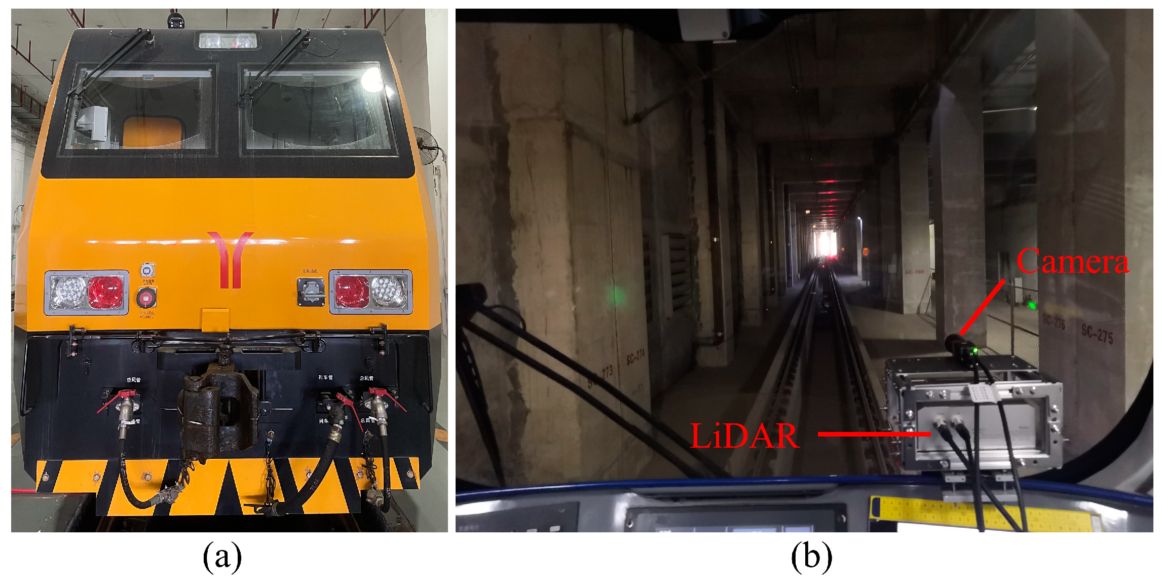
In this study, we initially trained a neural network on the RailSem19 dataset [21] to perform semantic segmentation of railway tracks. RailSem19 consists of a diverse set of 8500 railway scenes from 38 countries in varying weather, lighting, and seasons. Subsequently, LiDAR and camera data from railway scenarios were collected for railway track detection and 3D fitting experiments, using the Neuvition Titan M1-R LiDAR with a repetition rate of 1 MHz and a synchronized high-resolution Alvium G5-1240 camera with a resolution of 4024 × 3036, as shown in Figure 9. To examine the algorithm’s generalization to LiDAR, we conducted additional experiments by replacing the LiDAR in certain scenarios with Livox Tele-15, featuring a longer detection range but sparser point clouds.

We collected some static scenarios of the train on straight and curve tracks, as well as dynamic scenarios of the train moving at a speed of 10 km/h using the LiDAR and camera. We manually segmented the railway tracks as ground truth. Due to limitations in LiDAR performance, there are numerous noise points along the edges of the railway tracks. To address this, we struggled to segment the surface points on the railway track as the ground truth for railway track point cloud segmentation. We attached retroreflective tape and placed traffic cones alongside the railway tracks to obtain the ground truth for railway track detection and 3D fitting. In the straight track scenario, the semantic segmentation of railway tracks obtained from the camera extends up to 200 m, while the LiDAR railway track point clouds typically cover distances of no more than 50 m. In the curve track scenario, due to the increased reflectivity on the side of the railway tracks, LiDAR is capable of detecting tracks at the distance of around 80 m. Overall, the camera outperforms LiDAR in detecting railway tracks at a longer distance.

The camera and LiDAR data are processed on the NVIDIA Jetson AGX Orin, a computing platform designed for autonomous vehicles and intelligent machines, equipped with GPUs and AI accelerators. Leveraging this edge computing device, we aim to perform real-time processing of camera and LiDAR data to achieve railway track detection and 3D fitting.

4.2. Railway Track Point Cloud Segmentation

The accuracy of railway track point cloud segmentation is crucial for subsequent extrinsic parameter optimization, as it provides precise extrinsic parameters for inverse projection. Firstly, we describe the railway track point level evaluation indicators. If the segmented LiDAR points coincide with the ground truth of the railway track point clouds, then these points are considered true positives (TP). If the segmented LiDAR points do not belong to the ground truth of the railway track point clouds, then these points are considered false positives (FP). If the points from the ground truth of the railway track point clouds do not appear in the segmented LiDAR points, then these points are considered false negatives (FN). We choose precision, recall rate, and F1 score as evaluation metrics, as illustrated in Equations (12)–(14).

$$Precision=\frac{TP}{TP+FP}$$

(12)

$$Recall=\frac{TP}{TP+FN}$$

(13)

$$F1=2\times \frac{Precision\times Recall}{Precision+Recall}$$

(14)

It should be noted that, due to the presence of noise points along the edges of the railway tracks, for the sake of algorithm robustness, post processing is applied to obtain surface points on the railway tracks. This leads to a slight reduction in recall rate. In other words, we aim to maximize precision under the condition of a sufficiently high recall rate. The F1 score is used as the comprehensive evaluation metric for railway track point cloud segmentation.

We compared the proposed method with the existing LiDAR-based method [15] and camera–LiDAR fusion method [17]. Due to the generalization problem of these methods, it is difficult to apply these methods directly to our data. For a fair comparison, some adjustments were made to these methods. The LiDAR-based method initially filters track bed and track points based on the height of the point cloud. However, implementing this on our data is challenging since our LiDAR was not horizontally mounted. We use prior knowledge to obtain the ROI area of the track bed, followed by applying the RANSAC algorithm to perform plane fitting on the points within this area. Points not on the plane are then filtered, and these points mainly include the track points. Finally, the LiDAR-based method segments the track point clouds using clustering and region-growing algorithms. As for the camera –LiDAR fusion method, originally designed for obstacle detection, the LiDAR point clouds are projected onto the image. Using the semantic segmentation of the tracks, the LiDAR track point clouds are filtered out. The results of railway track point cloud segmentation obtained by our method and other methods are presented in

Table 1. Results of railway track point cloud segmentation.

Scenario	LiDAR-Based Method [15]			Wang et al. [17]			Proposed Method
	Pre	Rec	F1	Pre	Rec	F1	Pre	Rec	F1
Straight	0.922	0.935	0.928	0.714	0.915	0.802	0.986	0.940	0.962
Curve	0.876	0.500	0.634	0.512	0.847	0.637	0.930	0.749	0.828
Dynamic	0.939	0.811	0.870	0.519	0.524	0.521	0.999	0.905	0.950

Bold indicates the best-performing metric among the compared methods.

.

Compared with other methods, our method achieves the highest precision, recall rate, and F1 score in the straight and dynamic scenarios. In the curve scenario, our method exhibits the highest precision and F1, with a recall rate slightly lower than that of the camera–LiDAR fusion method. This difference in recall rate is attributed to our post processing of the railway track point clouds, where only the surface points on the tracks are retained. The LiDAR-based method lacks robustness, frequently encountering severe railway track segmentation errors in the curve and dynamic scenarios. The camera–LiDAR fusion method heavily relies on the accuracy of rail semantic segmentation, often misclassifying track bed points as track points. Additionally, changes in the extrinsic parameters of the camera and LiDAR result in decreased accuracy in railway track point cloud segmentation. Visualization results of some railway track point cloud segmentations are presented in Figure 10, indicating that our method achieves more accurate and robust railway track point cloud segmentation.

4.3. The 3D Fitting of Railway Tracks

The precise acquisition of the 3D track trajectory is crucial for train operational safety. We assess the 3D fitting of railway tracks at specific distances, using the lateral deviation from the ground truth as the evaluation metric. As illustrated in Equation (15), $x_{pred}^i$ and $x_{gt}^i$ represent the x-values of the 3D fitted curve and the ground truth of the railway track, respectively, at the specific z-value.

$$Lateral deviation=\left|x_{pred}^i-x_{gt}^i\right|,i\in special z\text{-}values$$

(15)

We compared the proposed method with a LiDAR-based method [15], a camera-based method [13], and a camera–LiDAR fusion method [17]. Due to limitations in LiDAR performance and the low reflectivity of the railway track surface, only the near track points are detectable, while the distant track points remain inaccessible. For a fair comparison, the railway track points segmented by the LiDAR-based method and camera–LiDAR fusion method are subjected to 3D fitting using Equation (6). This procedure extends the railway tracks to distant locations for a comprehensive evaluation. The camera-based method achieves railway track semantic segmentation by finding a homography transformation matrix and mapping it to the BEV. The 3D fitting results of railway tracks obtained by the proposed method and other methods are presented in

Table 2. Detailed 3D fitting results of railway tracks.

Distance (m)	Scenario	Lateral Deviation (m)
		LiDAR-Based Method [15]	Wang et al. [13]	Camera-Based Method [17]	Proposed Method
40	Straight	0.05	0.04	0.04	0.03
	Curve	0.03	0.04	0.03	0.02
	Dynamic	0.06	0.10	0.07	0.03
80	Straight	0.11	0.11	0.09	0.06
	Curve	1.06	0.10	0.09	0.08
	Dynamic	0.40	0.26	0.18	0.08
120	Straight	0.19	0.20	0.13	0.10
	Curve	5.25	0.33	0.15	0.14
	Dynamic	0.74	0.43	0.30	0.12
160	Straight	0.27	0.29	0.18	0.13
	Curve	9.61	0.70	0.19	0.17
	Dynamic	1.08	0.60	0.43	0.16
200	Straight	0.35	0.40	0.23	0.17
	Curve	13.91	1.07	0.25	0.22
	Dynamic	1.43	0.77	0.56	0.21

Bold indicates the best-performing metric among the compared methods.

.

Evidently, the proposed method outperforms the other methods in all scenarios, with the smallest lateral deviation in the 3D fitting of railway tracks. In the curve scenario, the proposed method significantly outperforms the LiDAR-based method and the camera–LiDAR fusion method. The LiDAR-based method and the camera–LiDAR fusion method struggle to accurately segment track point clouds in the curve scenario, leading to increasing errors in 3D fitting of railway tracks. In the dynamic scenario, the movement of the train induces changes in extrinsic parameters. This results in an increasing lateral deviation in the 3D fitting of railway tracks for the other three methods. In contrast, the proposed method demonstrates superior adaptability to the extrinsic parameter changes. The visualization results of the 3D fitting for railway tracks are shown in Figure 11, confirming the accuracy of the proposed method in 3D fitting of railway tracks.

These experiments depend on accurate semantic segmentation of railway tracks in the images. Subsequently, we investigated the algorithm’s robustness in challenging scenarios where precise semantic segmentation of railway tracks may not be attainable. Experiments were conducted to assess the robustness of railway track detection and 3D fitting in challenging scenarios, including low illumination, occlusion, and track switches. Due to the noticeable differences in color and reflectivity between the railway surface and the surrounding track bed, the semantic segmentation module for railway tracks can also function in low-illumination scenarios. However, its performance may decrease slightly, with an effective detection range of only approximately 100 m. Additionally, the semantic segmentation of the railway track might be coarse, encompassing some areas of the track bed. Occlusion can lead to discontinuity in the semantic segmentation of the railway tracks. The Track switch may result in a significant overlap between the left and right tracks in the vicinity of the railway switch point. The algorithm’s robustness in challenging scenarios is demonstrated in

Table 3. Results of robustness experiments for challenging scenarios.

Evaluation Metric	Low Illumination	Occlusion	Track Switch
Average lateral deviation (m)	0.06	0.07	0.25

and visualization results are presented in Figure 12.

We adopted the average lateral deviation within 100 m as the evaluation metric. It is evident that the proposed method maintains robust performance in these challenging scenarios. In low illumination and occlusion scenarios, the 3D fitting error of railway tracks is comparable to that in normal scenarios. In the track switch scenario, the 3D fitting error of railway tracks increases slightly, but it remains acceptable and the algorithm continues to operate stably.

These experiments were conducted on the edge computing device NVIDIA Jetson AGX Orin (NVIDIA, Santa Clara, CA, USA). In view of the requirement of real-time performance for practical application of the system, we strove to reduce the computational complexity of the algorithm and minimize computation time. We employed parallel computing and multi-threaded processing mechanisms, along with moderate downsampling of the experimental data, to strike a balance between accuracy and computational efficiency while ensuring the required precision. We divided the entire algorithm into four parts based on their computational time consumption, namely railway semantic segmentation, inverse projection and 3D fitting of railway tracks, railway point cloud segmentation, and extrinsic parameter optimization. Due to the adoption of multi-threaded processing mechanisms, the total processing time is not simply the sum of the individual module times, but slightly greater than the time taken by the module with the maximum consumption. The computational time of the entire algorithm is presented in

Table 4. Results of computational time of the proposed method.

Module	Time Cost (s)
Railway semantic segmentation	0.174
Inverse projection and 3D fitting of railway tracks	0.001
Railway point cloud segmentation	0.065
Extrinsic parameter optimization	0.129
Total	0.200

.

The modules with the highest computational time consumption in the entire algorithm are the railway semantic segmentation module and the extrinsic parameter optimization module. The railway semantic segmentation module involves the computation of the railway centerline, which is a time-consuming process. Similarly, the extrinsic parameter optimization module requires traversal operations, which also contribute significantly to the total processing time. With parallel computing, we can maintain the algorithm’s processing speed at around five frames per second (fps), meeting the real-time requirements effectively. As the maximum scanning rate of the LiDAR is 100 milliseconds, the real-time performance of the proposed method can roughly meet the requirements for practical applications.

4.4. Ablation Study

The proposed method involves three crucial modules that may influence the railway track detection and 3D fitting: extrinsic parameter optimization, railway track point cloud post processing, and 3D fitting constraints. To further investigate the impacts of these three modules on the algorithm, each module was independently removed in experiments for comparison purposes. Specifically, fixed extrinsic parameters were used instead of the extrinsic parameter optimization module, points within the ROI are directly considered as the final railway track points, and a conventional polynomial function was employed instead of the piecewise function with curve constraints.

The ablation experiments for railway track point cloud segmentation are presented in

Table 5. Ablation experiments for railway track point cloud segmentation.

Method	F1 Score
	Straight	Curve	Dynamic	All
W/o extrinsic parameter optimization	0.941	0.791	0.851	0.861
W/o railway track point cloud post processing	0.626	0.322	0.768	0.572
W/o 3D fitting constraints	0.961	0.479	0.948	0.796
Proposed method	0.962	0.828	0.950	0.913

Bold indicates the best-performing metric among the compared methods.

. We chose the F1 score as the evaluation metric. Evidently, the complete algorithm achieves the highest F1 score. When removing the extrinsic parameter optimization module, railway point cloud post processing module, and 3D fitting constraints module, the F1 score decreases by 6%, 43%, and 15%, respectively.

The ablation experiments for 3D fitting of railway tracks are presented in

Table 6. Ablation experiments for 3D fitting of railway tracks.

Method	Average Lateral Deviation (m)
	Straight	Curve	Dynamic	All
W/o extrinsic parameter optimization	0.10	0.19	0.33	0.21
W/o railway track point cloud post processing	0.15	0.67	0.23	0.35
W/o 3D fitting constraints	0.12	0.22	0.13	0.16
Proposed method	0.08	0.14	0.11	0.11

Bold indicates the best-performing metric among the compared methods.

. We adopted the average lateral deviation within 200 m as the evaluation metric. Evidently, the complete algorithm achieves the minimum detection error. When removing the extrinsic parameter optimization module, railway point cloud post processing module, and 3D fitting constraints module, the average lateral deviation increases by 88%, 218%, and 42%, respectively.

5. Conclusions

In this study, we propose a real-time railway track detection and 3D fitting method that integrates the camera and LiDAR data. Continuously optimizing the extrinsic parameters, we apply inverse projection and 3D fitting to the semantic segmentation of the track, achieving track vectorization. Experimental results demonstrate the desirable accuracy of the proposed method in both railway track point cloud segmentation and 3D fitting of railway tracks, outperforming existing LiDAR-based, camera-based, and camera–LiDAR fusion methods. The proposed method achieves a 91.3% F1 score for railway track point cloud segmentation and maintains the average lateral deviation of 0.11 m within the 200 m distance for 3D fitting of the railway tracks. Additionally, the proposed method demonstrates robust performance in challenging scenarios such as curved tracks, obstacle occlusion, and vibrations during the train’s operation. All these experiments help verify the effectiveness of the proposed method.

The railway track detection and 3D fitting in this study relies on semantic segmentation; future work will focus on iteratively enhancing the semantic segmentation of railway tracks through the utilization of railway track point clouds. Additionally, there will be an emphasis on improving the algorithm’s portability for deployment on edge devices.

References

- Minoru, A. Railway safety for the 21st century. Jpn. Railway Transp. Rev. 2003, 36, 42–47. [Google Scholar]
- Jesús, G.J.; Ureña, J.; Hernandez, A.; Mazo, M.; Jiménez, J.A.; Álvarez, F.J.; De Marziani, C.; Jiménez, A.; Diaz, M.J.; Losada, C.; et al. Efficient multisensory barrier for obstacle detection on railways. IEEE Trans. Intell. Transp. Syst. 2010, 11, 702–713. [Google Scholar]
- Martin, L.; Stein, D. A train localization algorithm for train protection systems of the future. IEEE Trans. Intell. Transp. Syst. 2014, 16, 970–979. [Google Scholar]
- He, D.; Li, K.; Chen, Y.; Miao, J.; Li, X.; Shan, S.; Ren, R. Obstacle detection in dangerous railway track areas by a convolutional neural network. Meas. Sci. Technol. 2021, 32, 105401. [Google Scholar] [CrossRef]
- Wang, T.; Zhang, Z.; Tsui, K.-L. A deep generative approach for rail foreign object detections via semisupervised learning. IEEE Trans. Ind. Inform. 2022, 19, 459–468. [Google Scholar] [CrossRef]
- Zheng, S.; Wu, Z.; Xu, Y.; Wei, Z. Intrusion Detection of Foreign Objects in Overhead Power System for Preventive Maintenance in High-Speed Railway Catenary Inspection. IEEE Trans. Instrum. Meas. 2022, 71, 2513412. [Google Scholar] [CrossRef]
- Wang, Z.; Wu, X.; Yu, G.; Li, M. Efficient rail area detection using convolutional neural network. IEEE Access 2018, 6, 77656–77664. [Google Scholar] [CrossRef]
- Wang, Y.; Wang, L.; Hu, Y.H.; Qiu, J. RailNet: A segmentation network for railroad detection. IEEE Access 2019, 7, 143772–143779. [Google Scholar] [CrossRef]
- Yang, Z.; Cheung, V.; Gao, C.; Zhang, Q. Train intelligent detection system based on convolutional neural network. In Advances in Human Factors and Simulation: Proceedings of the AHFE 2019 International Conference on Human Factors and Simulation, Washington, DC, USA, 24–28 July 2019; Springer International Publishing: Cham, Switzerland, 2020. [Google Scholar]
- Fatih, K.; Akgul, Y.S. Vision-based railroad track extraction using dynamic programming. In Proceedings of the 2009 12th International IEEE Conference on Intelligent Transportation Systems, St. Louis, MO, USA, 4–7 October 2009. [Google Scholar]
- Karakose, M.; Yaman, O.; Baygin, M.; Murat, K.; Akin, E. A new computer vision based method for rail track detection and fault diagnosis in railways. Int. J. Mech. Eng. Robot. Res. 2017, 6, 22–27. [Google Scholar] [CrossRef]
- Li, H.; Zhang, Q.; Zhao, D.; Chen, Y. RailNet: An information aggregation network for rail track segmentation. In Proceedings of the 2020 International Joint Conference on Neural Networks (IJCNN), Glasgow, UK, 19–24 July 2020. [Google Scholar]
- Yang, S.; Yu, G.; Wang, Z.; Zhou, B.; Chen, P.; Zhang, Q. A topology guided method for rail-track detection. IEEE Trans. Veh. Technol. 2021, 71, 1426–1438. [Google Scholar] [CrossRef]
- Wang, Z.; Yu, G.; Chen, P.; Zhou, B.; Yang, S. FarNet: An Attention-Aggregation Network for Long-Range Rail Track Point Cloud Segmentation. IEEE Trans. Intell. Transp. Syst. 2021, 23, 13118–13126. [Google Scholar] [CrossRef]
- Mostafa, A. Automated recognition of railroad infrastructure in rural areas from LiDAR data. Remote Sens. 2015, 7, 14916–14938. [Google Scholar] [CrossRef]
- Yang, S.; Wang, Z.; Yu, G.; Zhou, B.; Chen, P.; Wang, S.; Zhang, Q. RailDepth: A Self-Supervised Network for Railway Depth Completion based on a Pooling-Guidance Mechanism. IEEE Trans. Instrum. Meas. 2023, 72, 5018313. [Google Scholar] [CrossRef]
- Wang, Z.; Yu, G.; Wu, X.; Li, H.; Li, D. A camera and LiDAR data fusion method for railway object detection. IEEE Sens. J. 2021, 21, 13442–13454. [Google Scholar]
- Le Saux, B.; Beaupère, A.; Boulch, A.; Brossard, J.; Manier, A.; Villemin, G. Railway detection: From filtering to segmentation networks. In Proceedings of the IGARSS 2018-2018 IEEE International Geoscience and Remote Sensing Symposium, Valencia, Spain, 22–27 July 2018. [Google Scholar]
- Qi, Z.; Tian, Y.; Shi, Y. Efficient railway tracks detection and turnouts recognition method using HOG features. Neural Comput. Appl. 2013, 23, 245–254. [Google Scholar] [CrossRef]
- Bogdan Tomoyuki, N.; Ukai, M. A vision-based approach for rail extraction and its application in a camera pan–tilt control system. IEEE Trans. Intell. Transp. Syst. 2012, 13, 1763–1771. [Google Scholar]
- Zendel, O.; Murschitz, M.; Zeilinger, M.; Steininger, D.; Abbasi, S.; Beleznai, C. Railsem19: A dataset for semantic rail scene understanding. In Proceedings of the IEEE/CVF Conference on Computer Vision and Pattern Recognition Workshops, Long Beach, CA, USA, 15–20 June 2019. [Google Scholar]
- D’Amico, G.; Marinoni, M.; Nesti, F.; Rossolini, G.; Buttazzo, G.; Sabina, S.; Lauro, G. TrainSim: A railway simulation framework for LiDAR and camera dataset generation. IEEE Trans. Intell. Transp. Syst. 2023, 24, 15006–15017. [Google Scholar] [CrossRef]
- He, K.; Zhang, X.; Ren, S.; Sun, J. Deep residual learning for image recognition. In Proceedings of the IEEE Conference on Computer Vision and Pattern Recognition, Las Vegas, NV, USA, 27–30 June 2016. [Google Scholar]
- Cheng, Y.-J.; Qiu, W.-G.; Duan, D.-Y. Automatic creation of as-is building information model from single-track railway tunnel point clouds. Autom. Constr. 2019, 106, 102911. [Google Scholar] [CrossRef]
- Yang, B.; Fang, L. Automated extraction of 3-D railway tracks from mobile laser scanning point clouds. IEEE J. Sel. Top. Appl. Earth Obs. Remote Sens. 2014, 7, 4750–4761. [Google Scholar] [CrossRef]
- Tan, K.; Cheng, X.; Ju, Q.; Wu, S. Correction of mobile TLS intensity data for water leakage spots detection in metro tunnels. IEEE Geosci. Remote Sens. Lett. 2016, 13, 1711–1715. [Google Scholar] [CrossRef]
- Soilán, M.; Nóvoa, A.; Sánchez-Rodríguez, A.; Riveiro, B.; Arias, P. Semantic segmentation of point clouds with pointnet and kpconv architectures applied to railway tunnels. ISPRS Ann. Photogramm. Remote Sens. Spat. Inf. Sci. 2020, 2, 281–288. [Google Scholar] [CrossRef]
- Jiang, T.; Yang, B.; Wang, Y.; Dai, L.; Qiu, B.; Liu, S.; Li, S.; Zhang, Q.; Jin, X.; Zeng, W. RailSeg: Learning Local-Global Feature Aggregation with Contextual Information for Railway Point Cloud Semantic Segmentation. IEEE Trans. Geosci. Remote Sens. 2023, 61, 5704929. [Google Scholar] [CrossRef]
- Lou, Y.; Zhang, T.; Tang, J.; Song, W.; Zhang, Y.; Chen, L. A fast algorithm for rail extraction using mobile laser scanning data. Remote Sens. 2018, 10, 1998. [Google Scholar] [CrossRef]
- Lamas, D.; Soilán, M.; Grandío, J.; Riveiro, B. Automatic point cloud semantic segmentation of complex railway environments. Remote Sens. 2021, 13, 2332. [Google Scholar] [CrossRef]
- Caltagirone, L.; Bellone, M.; Svensson, L.; Wahde, M. LIDAR–camera fusion for road detection using fully convolutional neural networks. Robot. Auton. Syst. 2019, 111, 125–131. [Google Scholar] [CrossRef]
- Wang, J.; Wu, T.; Zheng, Z. LIDAR and vision based pedestrian detection and tracking system. In Proceedings of the 2015 IEEE International Conference on Progress in Informatics and Computing (PIC), Nanjing, China, 18–20 October 2015. [Google Scholar]
- Hwang, J.P.; Cho, S.E.; Ryu, K.J.; Park, S.; Kim, E. Multi-classifier based LIDAR and camera fusion. In Proceedings of the 2007 IEEE Intelligent Transportation Systems Conference, Bellevue, WA, USA, 30 September–3 October 2007. [Google Scholar]
- Rahman, M.; Liu, H.; Masri, M.; Durazo-Cardenas, I.; Starr, A. A railway track detection method using robotic vision on a mobile manipulator: A proposed strategy. Comput. Ind. 2023, 148, 103900. [Google Scholar] [CrossRef]
- Mahmoud, A.; Mohamed, M.G.; El Shazly, A. Low-cost framework for 3D detection and track detection of the railway network using video data. Egypt. J. Remote Sens. Space Sci. 2022, 25, 1001–1012. [Google Scholar] [CrossRef]
- Yu, C.; Gao, C.; Wang, J.; Yu, G.; Shen, C.; Sang, N. Bisenet v2: Bilateral network with guided aggregation for real-time semantic segmentation. Int. J. Comput. Vis. 2021, 129, 3051–3068. [Google Scholar] [CrossRef]
- Geiger, A.; Moosmann, F.; Car, Ö.; Schuster, B. Automatic camera and range sensor calibration using a single shot. In Proceedings of the 2012 IEEE International Conference on Robotics and Automation, Saint Paul, MN, USA, 14–18 May 2012. [Google Scholar]
- Cui, J.; Niu, J.; Ouyang, Z.; He, Y.; Liu, D. ACSC: Automatic calibration for non-repetitive scanning solid-state LiDAR and camera systems. arXiv 2020, arXiv:2011.08516. [Google Scholar]
- Martin, A.F.; Bolles, R.C. Random sample consensus: A paradigm for model fitting with applications to image analysis and automated cartography. Commun. ACM 1981, 24, 381–395. [Google Scholar]
Figure 1.
Framework of the proposed method. In the semantic segmentation result, red pixels represent the railway tracks and purple pixels represent the railway track area. In refined track points, green points are refined track points and red points are excluded points. In the final track detection and 3D fitting, green points represent LiDAR track points and red points represent the inverse projection.
Figure 2.
Railway track semantic segmentation. (a) Original image. (b) Segmentation results of the model. (c) Coarse segmented railway track. (d) Refined segmented railway track.
Figure 3.
Diagram of sensor installation position and coordinate systems.
Figure 4.
Diagram of camera side view.
Figure 5.
Pinhole camera model.
Figure 6.
Depiction of 3D fitting with piecewise functions.
Figure 7.
Railway track point cloud segmentation process. (a) demonstrates the coarse screening of railway track point clouds using the 3D fitted curve of inverse projection of tracks. (b) demonstrates the fine screening of railway track point clouds through dividing them into small sections. (c) demonstrates the selection of railway track points using the fitted plane of near railway track points, and (d) demonstrates the differences between segmented railway track points and ground truth. In (b,c), the green points represent railway track surface points, while the red points represent railway track side points or track bed points. In (b), the blue line represents the 3D fitted curve of inverse projection of railway track, and the dashed lines represent the boundaries of the intervals. In (d), the green points represent true positives, with the red points representing false positives and the blue points representing false negatives.
Figure 8.
Extrinsic parameter optimization diagram.
Figure 9.
Experimental platform. (a) Train. (b) Install position of sensors.
Figure 10.
Visualization results of railway track point cloud segmentation. The last three rows display the railway track point cloud segmentation results, with green points representing TP, red points representing FP, and blue points representing FN.
Figure 11.
Visualization results of 3D fitting for railway tracks. The last four rows display the 3D fitting results of railway tracks, with green points representing ground truth and red points representing predicted results.
Figure 12.
Visualization of robustness experiments for challenging scenarios.