Assessing Greenhouse Gas Monitoring Capabilities Using SolAtmos End-to-End Simulator: Application to the Uvsq-Sat NG Mission

Abstract

Monitoring atmospheric concentrations of greenhouse gases (GHGs) like carbon dioxide and methane in near real time and with good spatial resolution is crucial for enhancing our understanding of the sources and sinks of these gases. A novel approach can be proposed using a constellation of small satellites equipped with miniaturized spectrometers having a spectral resolution of a few nanometers. The objective of this study is to describe expected results that can be obtained with a single satellite named Uvsq-Sat NG. The SolAtmos end-to-end simulator and its three tools (IRIS, OptiSpectra, and GHGRetrieval) were developed to evaluate the performance of the spectrometer of the Uvsq-Sat NG mission, which focuses on measuring the main GHGs. The IRIS tool was implemented to provide Top-Of-Atmosphere (TOA) spectral radiances. Four scenes were analyzed (pine forest, deciduous forest, ocean, snow) combined with different aerosol types (continental, desert, maritime, urban). Simulated radiance spectra were calculated based on the wavelength ranges of the Uvsq-Sat NG, which spans from 1200 to 2000 nm. The OptiSpectra tool was used to determine optimal observational settings for the spectrometer, including Signal-to-Noise Ratio (SNR) and integration time. Data derived from IRIS and OptiSpectra served as input for our GHGRetrieval simulation tool, developed to provide greenhouse gas concentrations. The Levenberg–Marquardt algorithm was applied iteratively to fine-tune gas concentrations and model inputs, aligning observed transmittance functions with simulated ones under given environmental conditions. To estimate gas concentrations (CO₂, CH₄, O₂, H₂O) and their uncertainties, the Monte Carlo method was used. Based on this analysis, this study demonstrates that a miniaturized spectrometer onboard Uvsq-Sat NG is capable of observing different scenes by adjusting its integration time according to the wavelength. The expected precision for each measurement is of the order of a few ppm for carbon dioxide and less than 25 ppb for methane.

1. Introduction

Climate change represents one of the most significant challenges [1,2] of the 21st century. Its effects are increasingly evident, such as rising global temperatures, diminishing sea ice, glaciers and ice sheets melting, rising sea levels, and more frequent and severe heatwaves [3]. Increasing anthropogenic emissions, particularly from fossil fuel burning [4], have led to an unprecedented rise in the atmospheric concentration of greenhouse gases (GHGs), resulting in enhanced trapping of terrestrial infrared radiation and an unbalanced Earth’s Radiation Budget (ERB). This inflicts widespread impacts on the climate system, notably the global warming of the Earth’s surface, and poses a threat to the whole biosphere. In the face of a rapidly changing climate, global and comprehensive measurements of the Earth’s key climate variables are needed for studying the intricate dynamics of the climate and assessing the extent of human impact on the climate system. This knowledge is essential in formulating effective strategies for mitigation and adaptation and thus guiding us toward a more sustainable future. The Global Climate Observing System (GCOS) identifies 55 Essential Climate Variables (ECVs) that have to be monitored closely [5]. Since the anthropogenic emissions of carbon dioxide (CO₂) and methane (CH₄) are responsible for most of the global warming, their concentrations in the atmospheric columns are obviously key ECVs and their global monitoring from space is essential [6,7]. As an example, European Space Agency Climate Change Initiative (ESA CCI) focuses on measurements related to CO₂ and CH₄ in the context of climate change research and monitoring. It aims to provide comprehensive and accurate data on the concentrations of these GHGs in the atmosphere using satellite observations and other sources.

The monitoring of the two crucial GHGs, CO₂ and CH₄, must be conducted on multiple spatio-temporal scales to resolve the dynamics and cycles of GHGs in the atmosphere. For instance, we need observations with global coverage to characterize and understand the global distributions and trends of GHGs, but we also require high spatial resolution observations, ideally down to a few kilometers, to identify and quantify their local sources and sinks. Furthermore, we also need observations at relatively high temporal resolutions to resolve the strong diurnal variations in important GHG sources. Ideally, we should aim at carrying out continuous real-time observations on diurnal timescales over the entire globe. From this perspective, satellites emerge as central tools. One of the issues is the type of satellite and orbit most suited for the monitoring of GHGs. Satellites on Low Earth Orbit (LEO) are much closer to the Earth’s surface than Geostationary Orbit (GEO) satellites and hence can make observations at higher spatial resolutions over the entire globe including the polar regions. However, compared to GEO satellites, LEO satellites have a very limited field of view and do not observe the same scene continuously at all, with typically long revisit periods (time elapsed between observations of the same scene by a satellite). A way around these limitations of LEO satellites is a trailing satellite constellation. This configuration enables an overall shorter revisit period (time elapsed between observation of the same scene but here by different satellites of the train), thus resolving partially the short-term variability in the distributions of CO₂ and CH₄ all over the globe.

To reduce costs and implementation times, a SmallSat constellation is an attractive option. Indeed, SmallSat constellations have already proved their worth in the monitoring of ECVs, for example, in the ongoing measurements of the Earth Energy Imbalance (EEI) within the framework of Uvsq-Sat [8] and Inspire-Sat 7 [9] missions. Uvsq-Sat NG [10] is an innovative SmallSat designed to demonstrate the feasibility of measuring carbon dioxide and methane, with accuracies tending towards those of large satellite missions. The Uvsq-Sat NG mission is led by the Laboratoire Atmosphères, Observations Spatiales (LATMOS), a French laboratory specialized in climate and Earth atmosphere sciences. The launch of Uvsq-Sat NG is planned in 2025. This mission is viewed as a pathfinder in the near-real-time monitoring of GHGs with a SmallSat constellation. CO₂ and CH₄ measurements will be performed with a small and compact spectrometer [10]. The miniaturization of such an optical instrument has led to some compromises, especially concerning the spectral resolution of the spectrometer, which is approximately ∼5 nm. The light source of the Uvsq-Sat NG spectrometer is the solar spectrum backscattered upwards in the 1200–2000 nm wavelength range. The Uvsq-Sat NG spectrometer, with its linear complementary metal oxide semiconductor (CMOS) sensor containing 256 pixels, is designed to capture Earth observational scenes with a ground footprint diameter close to 5 km thanks to its 0.15° narrow field of view. Uvsq-Sat NG also includes a high-definition camera (NanoCam) designed to capture images of the Earth in the visible range. The inclusion of NanoCam plays a crucial role in the post-processing of data acquired through the NIR spectrometer. It ensures precise geolocation of observed scenes, aiding in the accurate analysis of data to distinguish measurements taken during clear-sky conditions from those acquired under cloudy conditions. Uvsq-Sat NG, equipped with its miniaturized payloads, is designed to serve as a forerunner for a future SmallSat constellation which will be capable of thorough and precise monitoring of fossil fuel emissions.

The aim of this paper is to assess the expected performances of the Uvsq-Sat NG spectrometer in measuring atmospheric columns of CO₂ and CH₄ through low spectral observations and its potential use in the identification of local emissions within the framework of a SmallSat constellation. This simulation-based evaluation is essential to confirm that the spectrometer can fulfill the scientific objectives. Section 2 outlines the importance of tracking GHGs and enumerates a few key space-based missions focused on CO₂ and CH₄ observations. This section also discusses the Uvsq-Sat NG’s mission in comparison with the capabilities of existing and upcoming space-based missions. Section 3 presents the general method used to validate the relevance of a miniaturized low-resolution spectrometer to reach the accuracy requirements in GHG observations. The SolAtmos end-to-end simulator was developed to assess the performances of space-based instruments aimed at monitoring GHGs, such as CO₂ and CH₄. This simulator integrates three tools—IRIS, OptiSpectra, and GHGRetrieval. These tools collectively facilitate the estimation of achievable accuracies across observational setups. SolAtmos is particularly relevant in the framework of the Uvsq-Sat NG mission, as this satellite is equipped with a Near-Infrared (NIR) spectrometer that operates at low spectral resolution. Section 4 presents the detailed simulation results, which are based on the input parameters of the Uvsq-Sat NG mission and its NIR miniaturized spectrometer. Section 5 delves into the potential applications and perspectives for this miniaturized spectrometer, discussing its limitations in certain observational setups and retrieval parameters. Finally, the results are used to identify the observation cases and spectrometer parameter settings for which Uvsq-Sat NG can reach the measurement requirements.

2. Relevance of GHG Observations and Scientific Requirements of a Few Space Missions

The rise in atmospheric GHG levels primarily caused by human activities has been identified as the principal factor behind the observed increase in Earth’s surface temperature. In 2023, set to be the warmest year on record, the global temperature increase reached 1.4 °C compared to pre-industrial era, breaking climate records. Predictions suggest that in 2024, it could exceed the 1.5 °C warming threshold for the first time—beyond the warming limit outlined by the Intergovernmental Panel on Climate Change (IPCC). This escalation might be partially attributed to an unexpectedly strong El Niño event, which leads to changes in wind patterns that distribute warm waters across the Pacific Ocean, resulting in a temporary atmospheric warming. This El Niño naturally occurring climate phase can impact global warming even more significantly depending on its intensity and resultant effect on temperatures. This phenomenon compounds the ongoing temperature rise associated with increasing GHGs.

Carbon dioxide is the foremost contributor to climate change and it represents a significant GHG primarily resulting from human activities. Its concentration in the atmosphere has risen from a pre-industrial level of approximately 280 parts per million (ppm) to over 420 ppm in 2024. This rise is attributed to sources including deforestation, changes in land use, cement manufacturing, and notably the combustion of fossil fuels. The latter became the predominant source of emissions around the 1950s [11], and currently accounts for over 87% of total emissions [12].

Atmospheric methane is the second largest contributor to climate change and consists of a diverse mix of overlapping sources and sinks, so it is difficult to quantify emissions by source type. Its concentration in the atmosphere has risen from a pre-industrial level of approximately ∼720 parts per billion (ppb) to over 1900 ppb in 2024. Since 2007, globally averaged atmospheric methane concentration has been increasing at an accelerating rate. The annual increases in 2020 and 2021 (15 and 18 ppb, respectively) are the largest since systematic record began in 1983. Causes are still being investigated and analysis indicates that the largest contribution to the renewed increase in methane since 2007 comes from biogenic sources, such as wetlands or rice paddies.

Quantifying CO₂ and CH₄ variations and anthropogenic emissions is critical for understanding the current and future impact of human activities on climate change. It is also vital to track global emissions across the entire planet, not just in mid-latitude regions. Monitoring at the poles is particularly important due to the significant climate changes occurring there. For instance, the melting of Arctic ice releases substantial amounts of methane previously trapped within the ice. Additionally, it is necessary to measure GHG emissions as comprehensively as possible across the globe at different geographic scales. Depending on the spatial resolution, it is feasible to monitor GHG sources and sinks on larger regional scales, such as for national GHG assessments, in megacities, or even at point sources smaller than a few kilometers. The deployment of space-based instruments is indispensable for global GHGs monitoring, providing the breadth of coverage required to accurately track these emissions worldwide.

ESA CCI recommends space-based instruments to achieve a 1 ppm absolute accuracy in measuring the CO₂ total column, with a precision of 1 ppm and a stability per decade of 2 ppm. Meeting these requirements enables near-real-time sink determination with a spatial resolution of 5 km and a revisit time of 3 h. Regarding CH₄ total column measurements, the recommended requirements include 2 ppb absolute accuracy, 5 ppb precision, 2 ppb stability per decade, 10 km spatial resolution, and a revisit time of 3 h. Numerous space-based missions were deployed with the primary objective of measuring the atmospheric columns of greenhouse gases (

Table 1. Scientific requirements of a few key space-based missions.

Satellite/Instrument	Satellite Type	Operational Period	XCO2 Accuracy	XCH4 Accuracy	References
SCIAMACHY	Large	2002–2012	1.2 ppm	20 ppb	[13]
GOSAT	Large	2009–Present	2 ppm	13 ppb	[14]
OCO-2	Large	2014–Present	0.65 ppm	/	[15]
GHGSat	SmallSat	2016–Present	4.2 ppm	95 ppb	[16]
TROPOMI	Large	2017–Present	/	<20 ppb	[17]
Uvsq-Sat NG	SmallSat	No earlier than 2025	4 ppm	25 ppb	[10]
MicroCarb	MicroSat	No earlier than 2025	<0.2 ppm	/	[18]
Merlin	Large	No earlier than 2028	/	3.7 ppb	[19]

). These missions aim to gather comprehensive data on the concentration and distribution of GHGs like CO₂ and CH₄ in the Earth’s atmosphere.

Scanning Imaging Absorption Spectrometer for Atmospheric Chartography (SCIAMACHY) onboard ENVIronment SATellite (ENVISAT) was one of the earlier instruments to make global observations of greenhouse gases and was significant for its ability to measure the concentration of these gases over both land and ocean. From 2002 and over the span of a decade, the SCIAMACHY instrument [20] conducted global measurements of trace gases in both the troposphere and the stratosphere with a relative accuracy for monthly averages within a 500 km radius of 1.2 ppm for the retrieval of CO₂ concentrations and 20 ppb for CH₄ concentrations [13]. These measurements were derived from the instrument’s capability to observe transmitted, back-scattered, and reflected radiation within the Earth’s atmosphere, across a broad wavelength spectrum ranging from 240 nm to 2400 nm. The spatial resolution of SCIAMACHY, at 30 × 60 km², limited its ability to pinpoint local point sources of emissions, except for those that were highly intense. Despite this, it was among the pioneering instruments to detect anthropogenic CO₂ emissions at a regional scale from space. The key emission zones identified included expansive regions such as Northern Europe, the East Coast of the United States, and China [21]. To effectively observe local sources and sinks of emissions, minimizing the ground footprint of the instrument is crucial.

Launched in January 2009, the Greenhouse Gases Observing Satellite (GOSAT) was the world’s first satellite designed specifically to monitor greenhouse gases from space. It primarily focuses on measuring the concentrations of CO₂ and CH₄. The mission aims to improve the accuracy of climate change predictions by providing detailed and global observations of these key greenhouse gases. GOSAT [14] equipped with its Thermal and Near-Infrared Sensor for Carbon Observation Fourier Transform Spectrometer (TANSO-FTS) features a spatial resolution with a 10.5 km diameter footprint. This resolution, combined with the satellite’s orbit, allows for the measurement of XCO₂ and XCH₄ (concentration averaged over the whole vertical atmospheric column) at the scale of megacities, with a ground-track repeat cycle occurring every 3 days.

Orbiting Carbon Observatory-2 (OCO-2) represents another key mission focused on observing greenhouse gases, and it stands out as one of the most accurate in GHG monitoring. Since 2014, OCO-2 [15] provides a global picture of CO₂ levels in the atmosphere, measuring both natural and anthropogenic sources of CO₂, as well as the variation of these sources over time. This satellite has the capability to detect local CO₂ point sources with a resolution of approximately 2 km, achieving outstanding accuracy below 0.65 ppm. However, its 16-day revisit cycle (https://ocov2.jpl.nasa.gov/, accessed on 6 September 2023) limits the feasibility of near-real-time CO₂ monitoring. Addressing this limitation, its successor, OCO-3, was mounted in 2019 on the International Space Station (ISS), providing enhanced coverage of mid-latitudes where human activities are more concentrated.

In 2016, the first small satellites dedicated to the observation of GHGs were launched with the primary goal of enhancing revisit time. These satellites, named GHGSat, have the mission of providing high-resolution, local-scale measurements of CO₂ and CH₄ emissions. The spatial and temporal resolution planned for such a constellation is impressive, but it is worth noting that the measurement accuracy of GHGSat is notably lower than that provided by larger satellites (Table 1).

The TROPOspheric Monitoring Instrument (TROPOMI) is another satellite specifically designed for monitoring Earth’s atmosphere and delivering highly accurate data on a range of atmospheric components, including total columns of carbon monoxide (CO) and CH₄.

Uvsq-Sat NG, set to launch in 2025, has a primary mission of providing precise and consistent measurements of greenhouse gases over time. Uvsq-Sat NG is focused on achieving absolute measurements of CO₂ within ±4.0 ppm with an annual stability of ±1.0 ppm. For CH₄, it aims for absolute measurements within ±25.0 ppb and an annual stability of ±10.0 ppb (Table 1). To calibrate and validate its greenhouse gas observations, Uvsq-Sat NG relies on the Total Carbon Column Observing Network (TCCON), which serves as the reference network for satellite data.

MethaneSAT was launched in March 2024 and represents a groundbreaking mission to protect the climate. There are also several other space missions currently under development dedicated to GHG observations, such as GOSAT-3 (2024), MicroCarb (2025), CO2M (2025), and Merlin (2028).

Achieving accurate greenhouse gas retrievals is a vital consideration for all these space-based missions. It entails the detection of incredibly subtle concentration variations, approximately 0.2% for XCO₂ and 0.5% for XCH₄. This accuracy depends on multiple factors, including instrument specifications, observational circumstances, as well as the development of data analysis techniques and new methods as shown in Section 3.

3. Methods for Evaluating the Performances of GHG Instruments Using SolAtmos

An end-to-end simulator named SolAtmos was developed to assess the performances of Uvsq-Sat NG [10]. Figure 1 illustrates the general implemented method. SolAtmos consists of three tools (IRIS, OptiSpectra, and GHGRetrieval) to enable the simulation of radiance datasets and the evaluation of the performances of several geophysical and instrumental parameters in estimating atmospheric gas columns, including CO₂, CH₄, O₂, and H₂O, as well as the associated uncertainties. SolAtmos is particularly valuable for determining the expected performance of space missions focused on observing GHG, and using the Sun as the primary source of illumination. It ensures XCO₂ accuracy at levels under 4 ppm and XCH4 under 25 ppb for the Uvsq-Sat NG mission, complying with scientific requirements (Table 1). It is capable of fulfilling the requirements for the Uvsq-Sat NG NIR spectrometer, which operates in the 1200–2000 nm spectral range with a low spectral resolution of ∼5 nm. SolAtmos uses fast and moderately spectrally resolved radiative transfer simulations, suitable for broad analysis across a wide array of geophysical and instrumental parameters. Additionally, it provides slower but highly resolved radiative transfer simulations for in-depth examination of specific and selected configurations. The steps carried out with SolAtmos are described below.

The first step is to determine radiances at Top Of Atmosphere (TOA). The IRIS tool is used to simulate a wide range of scenarios, taking into account parameters related to the Sun, atmosphere, surface, and instrumentation. Using these parameters, IRIS calculates and provides spectral radiances data at TOA for surface observational scenes (pine forest, deciduous forest, ocean, homogeneous snow).

The second step consists of modeling the opto-radiometric performances of the instrument. The OptiSpectra tool takes the spectral radiances data obtained from IRIS as input. It then models the entire optical path, taking into consideration elements such as optical characteristics and sensor parameters. OptiSpectra calculates critical performance metrics, including magnification of the instrument’s entrance slit on the sensor, Point-Spread-Function (PSF) of each monochromatic wave, radiometric performances, number of electrons for each pixel on the sensor, saturation of the sensor, slit functions, spectral resolution, and Signal-to-Noise Ratio (SNR). These metrics provide valuable insights into the instrument’s performance and the quality of measurements.

The third step is to retrieve the atmospheric gas concentrations and its uncertainties. GHGRetrieval uses the outputs from both IRIS (spectral radiances data) and OptiSpectra (performance metrics). It also uses input parameters that originate from the Sun, the atmosphere, and the instrument. GHGRetrieval is based on Levenberg–Marquardt algorithms and models to retrieve the concentrations of CO₂, CH₄, O₂, and H₂O. GHGRetrieval provides accurate and precise estimates of gas concentrations, making it a crucial tool for environmental monitoring and scientific research. The retrieved gas concentration values can be used for several applications, such as climate studies and air quality assessment, based on the comprehensive data obtained through the previous steps.

The SolAtmos approach is centered on a detailed process that considers a wide range of parameters from the observation conditions to the instrument’s performance. In subsequent sections, a more detailed explanation of the three tools used in the end-to-end simulator is provided.

3.1. Determining Radiances at TOA Using the IRIS Tool

IRIS is designed to mimic the alterations that the solar spectrum experiences as it passes through the atmosphere, beginning with the solar spectrum as it initially enters the atmosphere and continuing up to the point where it reaches the entrance of the instrument at TOA. IRIS relies on radiative transfer models, which help in understanding how solar radiation interacts with different components of the Earth’s atmosphere, including gases, aerosols, and clouds. There are several radiative transfer codes available.

Table 2. General parameters of some Radiative Transfer Models (RTMs).

RTM	Spectral Range 1	Spectral Accuracy	Atmospheric Geometry 2	References
6S/6SV	VIS–NIR	2.5 nm	PP	[22]
SCIATRAN	UV–FIR	<0.2 nm on VIS and NIR	PP/PS/S	[23]
4A/OP	NIR–FIR	0.005 cm−1	/	[24]
DART	VIS–FIR	1 cm−1	S	[25]
LBLRTM	VIS–LWIR	Line-by-line	S	[26]
MODTRAN6	UV–LWIR	0.2 cm−1	PP	[27]
Eradiate	VIS–NIR	Line-by-line, 1 nm, 10 nm	PP/S	https://www.eradiate.eu/
LibRadTran	UV–FIR	0.05 to 1 nm (MWIR)	PP/S	[28]

¹ Spectral Range: Ultra-Violet (UV)—10 to 380 nm, Visible (VIS)—380 to 780 nm, Near-InfraRed (NIR)—780 to 3000 nm, Mid-Wave InfraRed (MWIR)—3 to 8 μm, Long-Wave Infrared (LWIR)—8 to 15 μm, Far Infrared (FIR)—15 to 1000 μm. ² Atmospheric Geometry: Parallel Plane (PP), Pseudo-Spherical (PS), Spherical (S).

presents the radiative transfer codes that can be used. The radiative transfer codes Second Simulation of Satellite Signal in the Solar Spectrum Vector (6SV) and SCIATRAN are used because they have the ability to conduct fast and moderately resolved (spectrally) radiative transfer simulations in the case of the former and highly resolved simulations in the case of the latter.

The Py6S Python wrapper of 6SV [22,29] and SCIATRAN radiative codes were therefore selected and integrated into the IRIS tool.

6SV, developed by the Laboratoire d’Optique Atmosphérique (LOA, Lille, France), enables calculations for space and airborne observations in VIS to SWIR for nadir conditions (downward-oriented line of sight), taking into account target elevation, surface conditions, and absorbing species. The 6SV code simulates radiative transfer in the 400–2500 nm range with a spectral resolution of 2.5 nm, which represents a wavelength range compatible with the definition of the Uvsq-Sat NG spectrometer.

6SV is therefore particularly useful in the context of this mission because it also allows generation of a large sets of spectra covering a multitude of geophysical conditions. However, the 6SV simulations at 2.5 nm resolution are not finely detailed enough to simulate TOA spectra accurately. They serve a more general purpose, typically for providing rough estimates, especially when assessing the characteristics of different scenes that are encountered. To address this lack of precision, SCIATRAN, developed by the Institute of Environmental Physics (University of Bremen, Germany), is used with a line-by-line mode that utilizes the High-Resolution Transmission (HITRAN) database [30] for highly precise and comprehensive simulations. It covers a wide spectral range from 175 to 40,000 nm, supports Parallel Plane, Pseudo-Spherical, and Spherical geometries (Table 2), and all lines of sight from nadir to limb. It models the vertical inhomogeneities of the atmosphere (temperature, pressure, concentrations, aerosols, and clouds) and includes scattering models and databases of optical properties of aerosols and clouds. SCIATRAN is designed for precise and high-resolution spectral simulations with a resolution of 0.2 nm in the 1070–1800 nm range [23]. This is essential for detailed studies of specific atmospheric phenomena or remote sensing applications where fine spectral details are crucial. Using the 6SV and SCIATRAN codes, IRIS thus simulates radiative transfer for obtaining TOA radiances at the instrument’s entrance, as well as total atmospheric transmissions.

The main inputs of the IRIS parameter are a set of solar conditions (solar spectrum, Solar Zenith Angle (SZA), etc.), geometric conditions (viewing angles), atmospheric conditions (molecular and aerosol composition), surface conditions (surface type and the Bidirectional Reflectance Distribution Function (BRDF) model), and instrumental conditions (slit functions, SNR, etc.). IRIS is used to generate instrumental responses with Gaussian or Voigt functions and applied to TOA radiance spectra.

The set of simulations required to evaluate the effect of these parameters and their values is determined by the Design Of Experiment (DOE) builder. It is possible to create a complete experimental design that tests each value of each parameter against each value of every other parameter. These exhaustive experimental designs test all possible combinations but require a large number of simulations (depending on the number of parameters and values to explore) and may not always be meaningful.

The IRIS tool can also be improved to take into account the complexity of the observed scenes such as those found in human activity areas like industrial zones, megacities, and landfills. DART [25,31] could be used for this purpose, taking advantage of its capability to simulate highly complex observation scenes effectively.

Finally, polarization of light within radiative transfer was not taken into account in the IRIS tool, even though the 6SV code has the capability to do so. First, it is because the Uvsq-Sat NG NIR spectrometer is not designed for observing light polarization or measuring associated Stokes polarization states. Furthermore, it is established that polarization in the NIR range has negligible effects on measurements [32].

3.2. Modeling the Opto-Radiometric Performances with the OptiSpectra Tool

The OptiSpectra tool is used to determine the optical and radiometric performances of a space instrument. The first step of the process involves designing the optical architecture of the space instrument using Zemax OpticStudio software [33]. It works by ray tracing, a method that simulates the propagation of the radiance at TOA within the space instrument. To characterize the performances of the Uvsq-Sat NG spectrometer, the Zemax OpticStudio optical design program is used. Figure 2 shows the optical configuration of this space instrument, which is close to an Ebert–Fastie-type grating spectrometer. It is a specific design of a spectrometer that uses a single parabolic mirror for both collimating and focusing light (source), combined with a diffraction grating (300 groves per mm) for dispersing light into its constituent wavelengths to the the focal surface (Indium Gallium Arsenide (InGaAs) linear CMOS image sensor of 256 pixels equipped with a Peltier thermoelectric cooler). The optical filter located at the entrance of the spectrometer is designed to transmit specific portions (1200–2000 nm) of the radiance at TOA. The entrance telescope (lens doublet) enhances the spectrometer’s capacity, thereby improving its resolution and broadening its field of view. Thanks to the lens doublet, the telescope PSF on the entrance slit has a resolution that is negligible in the overall contribution of the system aberrations. The entrance slit plays a crucial role in defining the spectrometer’s resolution and overall performance. It impacts the Uvsq-Sat NG spectrometer resolution, sensitivity, and the overall quality of the spectral data that are obtained in orbit. The choice of the entrance slit size and shape is a compromise between resolution and sensitivity, which represents an important point for obtaining the most accurate GHG observations.

Numerous inputs, such as the optical parameters depicted in Figure 1 for the OptiSpectra tool, are crucial for evaluating specific optical characteristics of the Uvsq-Sat NG NIR spectrometer, like PSF and magnification. The analysis through Zemax OpticStudio simulations therefore provides the PSF for each monochromatic wavelength and the magnification of the entrance slit on the sensor at the focal surface. The resolution of the instrument is closely linked to the PSF, thus enabling the Zemax OpticStudio simulation to ascertain the spectrometer’s slit functions. Additionally, the magnification of the entrance slit on the sensor is used to determine the optical extent of the instrument optical system. The optical extent characterizes the propagation of the light in the whole spectrometer according to the geometry of the optical system. It is a vital parameter for conducting radiometric analyses and performances, which represent the second step in the process implemented through the OptiSpectra tool.

The radiometric performances of the Uvsq-Sat NG spectrometer (number of electrons, saturation, slit functions, spectral resolution, SNR) were determined from the sensor’s characteristics. Equation (1) describes the number of electrons detected by the Uvsq-Sat NG spectrometer’s sensor based on the input parameters described above.

$$N_{e^{-}}(\lambda ,\tau )=S\left(\lambda \right)\times I_{\lambda }\left(\lambda \right)\times G\left(\lambda \right)\times \Delta \lambda \times \eta \left(\lambda \right)\times \tau$$

(1)

where $N_{e^{-}}$ is the number of electrons detected by the sensor, $\lambda$ is the wavelength (nm), S is the sensor sensitivity (e⁻ J⁻¹), $I_{\lambda }$ is the spectral radiance at TOA calculated with the IRIS tool (Wm⁻²sr⁻¹nm⁻¹), G is the geometrical extent (m²sr) that is an important parameter that influences the spectral resolution and defines the instrument’s field of view, $\Delta \lambda$ represents the considered spectral range (∼800 nm), $\eta$ is the global transmission of the instrument and $\tau$ is the integration time (s).

The quality of measurements performed by the Uvsq-Sat NG spectrometer depends strongly on the SNR. Indeed, a high SNR ratio is crucial for spectrometers and instruments used in GHG observations because it directly impacts the accuracy, sensitivity, and reliability of the data, which are essential for addressing climate change. The OptiSpectra tool allows for accurately determining the SNR for each simulation based on sensor characteristics. The primary sources of noise considered include reading noise, dark current, and electron noise. Equation (2) illustrates that SNR is influenced by several key factors such as integration time. For instance, as integration time increases, dark current noise also increases. Temperature is another parameter that affects SNR. Therefore, the sensor of the Uvsq-Sat NG spectrometer is thermally controlled in orbit to maintain a temperature (T) close to −20 °C in order to mitigate certain harmful effects.

$$\mathrm{SNR}(T,\tau ,\lambda )=\frac{N_{e^{-}}(\lambda ,\tau )}{\mathcal{N}(T,\tau ,\lambda )}$$

(2)

where $\mathcal{N}(T,\tau ,\lambda )$ represents the noise of measurements at a given wavelength ($\lambda$).

Measurement noise is defined as the global contribution of different noises. For high radiance, the main noise is electron noise ${\mathcal{N}}_{e^{-}}$, which is defined as the square root of signal $N_{e^{-}}$. The total noise also depends on the sensor’s characteristics and properties. For the Uvsq-Sat NG sensor, the two main noises are the ${\mathcal{N}}_{DC}$ dark current noise, defined in Equation (3), and the ${\mathcal{N}}_{RN}$ reading noise, which is a constant noise independent from incident flux or observation conditions (∼3125 e⁻).

$${\mathcal{N}}_{DC}(T,\tau )=\sqrt{\frac{I_{DC}\left(T\right)}{e}\times \tau }$$

(3)

where ${\mathcal{N}}_{DC}$ is the dark current noise, $I_{DC}$ is the dark current (A) at temperature T (K), e is the charge of an electron (C) and $\tau$ the integration time of the sensor (s). This noise is highly dependent on observation conditions, in particular sensor temperature. The chosen InGaAs sensor is cooled to limit the effects of dark current variations on the measurement.

The global noise ($\mathcal{N}$) is defined in Equation (4),

$$\mathcal{N}(\lambda ,T,\tau )=\sqrt{{\mathcal{N}}_{RN}^2+{\mathcal{N}}_{DC}^2(T,\tau )+{\mathcal{N}}_{e^{-}}^2(\lambda ,\tau )+{\eta }^2}$$

(4)

where $\eta$ represents all noise contributions not listed previously. It is assumed to be negligible compared to the noises described above.

According to Equations (1) and (4), the SNR increases with the integration time; however, $\tau$ cannot be indefinitely increased due to the full-well capacity of the sensor. If the electron flux is too high, the sensor will saturate. The full-well capacity does not vary with the wavelength, so saturation depends only on the integration time and temperature, as described in Equation (5).

$${\mathrm{SNR}}_{saturation}(T,\tau )=\frac{Q_{max}}{\mathcal{N}(T,\tau )}$$

(5)

where $Q_{max}$ is the full-well capacity of the sensor (17.5 Me⁻).

The OptiSpectra tool is used for determining the number of electrons ($N_{e^{-}}$) detected by the sensor of the Uvsq-Sat NG NIR spectrometer, its spectral SNR, saturation level, spectral resolution, and slit functions.

3.3. Retrieving Atmospheric Gas Concentrations and Uncertainties Using GHGRetrieval

GHGRetrieval represents the final tool used in the end-to-end SolAtmos simulator toolchain. This stage is essential for retrieving XCO₂ and XCH₄ concentrations from the radiance at TOA. With a spectral SNR and the spectral resolution of the instrument as inputs, the GHGRetrieval tool determines the atmospheric composition of CO₂, CH₄, H₂O, and O₂ concentrations. The whole methodology of GHGRetrieval is described in [10]. The first step is to normalize and convolve the atmospheric radiance at TOA with the spectral resolution of the Uvsq-Sat NG spectrometer. Then, the total dimensionless resulting transmittance function is determined, which depends on the gas mixing ratio in the atmospheric column. Next, the method uses the Levenberg–Marquardt algorithm to determine the concentrations of the four gases (CO₂, CH₄, O₂, H₂O) as they would be observed by the Uvsq-Sat NG spectrometer. Other methods can be used to obtain GHG concentrations. However, the Levenberg–Marquardt method is widely used in the atmospheric remote sensing community. It has the advantage of fully taking into account the variance–covariance matrices and averaging kernels between the different absorbing gases present in the atmosphere [34]. Finally, estimation of uncertainties in the concentration determination of the four gases is calculated using the Monte Carlo method.

The GHGRetrieval tool is suitable when we intend to retrieve atmospheric gas column concentrations (CO₂, CH₄, O₂, H₂O) from TOA radiance over a broad spectral range, such as between 1200 and 2000 nm, as exemplified by the Uvsq-Sat NG NIR spectrometer. Within the scope of the Uvsq-Sat NG mission, CO₂ displays absorption bands at approximately 1433, 1573, 1603, 1883, 1958, and 2000 nm. These bands capture radiation emitted by the Sun and reflected by the Earth, carrying the distinct signature of CO₂ molecules. Information about CO₂ concentration is contained within the depth of the disjointed absorption bands from those of other GHGs. CH₄ has two absorption bands of interest centered around 1645 and 1667 nm. O₂ exhibits a very strong absorption band around 1270 nm. This wavelength band serves two important purposes: it allows for the normalization of CO₂ and CH₄ concentration measurements while accounting for atmospheric pressure, and they consider the influence of scattering elements like clouds and aerosols. The 1.27 μm O₂ band is affected by the presence of O₂ airglow emission that adds some radiance in the center of O₂ absorption lines. If it is not taken into account, the estimation of the atmospheric pressure, proportional to the O₂ vertical column, will be underestimated. A study from 2020 [35] showed that the use of a priori airglow emission estimated by the Reactive Processes Ruling the Ozone Budget (REPROBUS) chemistry transport model reduces the bias on atmospheric pressure to less than 0.01% (0.1 hPa). Finally, H₂O displays several large significant absorption bands, including those around 1400 nm (ranging from ∼1280 to 1560 nm) and 1900 nm (extending from ∼1690 nm and beyond 2000 nm). Since the absorption bands of different gases are not all identical, it is possible to characterize the concentrations of each of them using the GHGRetrieval tool.

The GHGRetrieval’s process relies on simulated spectra encompassing a wide range of environmental conditions, including surface pressure, surface reflectance, vertical temperature profiles, mixing ratios of key gases, water vapor content, concentrations of other trace gases, cloud properties, and aerosol optical depth distributions. Additionally, it takes into account spectrometer characteristics, such as varying SNR across wavelengths and spectral resolutions in ranges starting from from few nanometers. However, if the objective is to directly observe specific, narrow, and unique spectral bands associated with greenhouse gases, the GHGRetrieval method may not be applicable. It must be tailored to enable the most accurate assessment of a single GHG observed at very high spectral resolution and within a very narrow band.

The GHGRetrieval tool can be enhanced to fulfill high-resolution requirement, utilizing its integration with the IRIS tool and based on the radiative transfer model SCIATRAN (Figure 3).

4. Results—Application to the Uvsq-Sat NG Mission

The simulations carried out with SolAtmos are intended to verify whether the Uvsq-Sat NG NIR spectrometer fulfills its scientific objectives as detailed in Table 1. This satellite is tasked with the global measurement of XCO₂ and XCH₄ to detect and quantify sources and sinks of greenhouse gases, a task that presents considerable challenges.

Sixteen scenarios are examined for different types of aerosols (continental, desert, maritime, and urban) and targeted surface (pine forest, deciduous forest, ocean, and homogeneous snow) with a solar zenith angle of 20°. Additionally, another sixteen scenarios are studied for different SZAs (0°, 20°, 50°, and 70°) and types of aerosols (continental, desert, maritime, and urban), with a surface targeted specifically for a pine forest.

For all simulations aimed at retrieving the concentrations of gases observable through the Uvsq-Sat NG NIR spectrometer, we assume a constant mixing ratio. While absorption by CO₂ and CH₄ may be influenced by the atmospheric profile, including variations in pressure and temperature that affect the intensity and width of CO₂ – CH₄ absorption lines, the impact of line broadening on Uvsq-Sat NG measurements is expected to be minimal. This is due to the instrument’s low spectral resolution, which prevents the resolution of individual absorption lines. In the future, it will be necessary to investigate the effect of the vertical profile’s shape on the estimation of CO₂ and CH₄ quantities, particularly for detecting sources where the concentration increases primarily in the lower layers of the atmosphere.

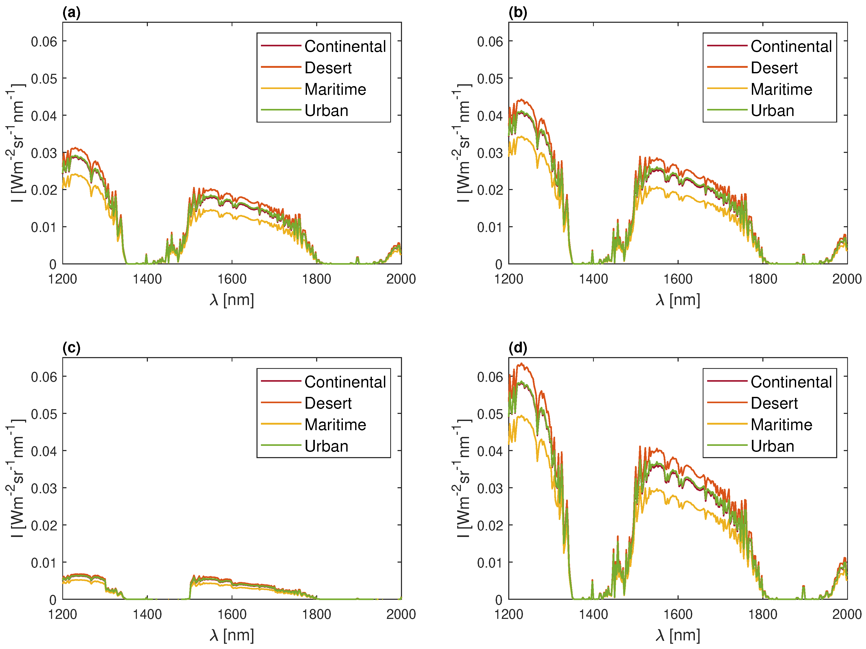
4.1. Evaluation of the Uvsq-Sat NG Radiance at TOA

Assessing the performances of the Uvsq-Sat NG spectrometer begin with calculating the observable radiances at TOA. The results associated with the 32 scenarios studied are presented in Figure 4 and Figure 5. Observable radiances at TOA strongly depend on the types of aerosols and the targeted surface. Observable radiances at TOA for ocean are low, which makes it difficult to determine GHG for this type of target surface.

Furthermore, the IRIS simulations did not take into account the satellite’s pointing errors thanks to the exceptional expected performance of Uvsq-Sat NG. The satellite is anticipated to have an absolute pointing error of less than 0.10° in all three axes and a drift error of less than 0.02°. It operates in a nadir pointing mode to maximize flux collection and minimize the ground footprint during its observations.

4.2. Evaluation of the Uvsq-Sat NG Opto-Radiometric Performances

The evaluation of the opto-radiometric capabilities of the Uvsq-Sat NG spectrometer was conducted using the OptiSpectra tool within SolAtmos, as outlined in Section 3. This tool facilitates the measurement of several opto-radiometric parameters specific to the Uvsq-Sat NG NIR spectrometer. The PSF and magnification of the Uvsq-Sat NG spectrometer were calculated. Additionally, the number of electrons was determined for each of the 32 scenarios, along with saturation levels, slit functions, spectral resolution, and SNR.

The SNR is primarily determined by the Uvsq-Sat NG NIR spectrometer sensor’s characteristics and the incoming radiance (Figure 4 and Figure 5), both of which are fixed parameters. One way for the spectrometer to modulate its SNR is by adjusting the integration time of its sensor.

Within the context of the Uvsq-Sat NG mission, a sensor integration time of 200 ms seems to be optimal for each of the 32 studied scenarios. This parameter allows for the determination of the number of electrons for each of the 32 radiances determined at TOA and shown in Figure 4 and Figure 5.

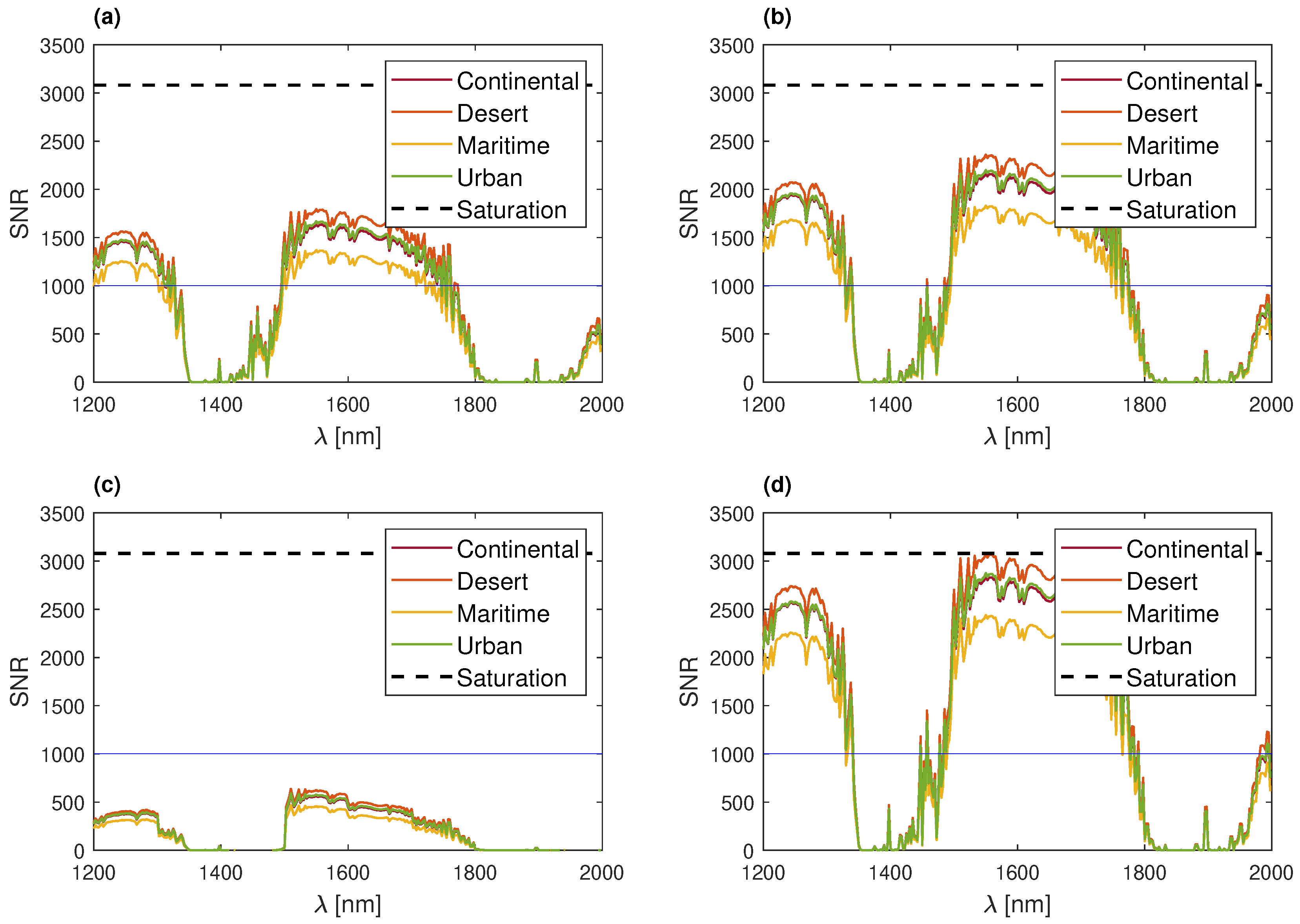
Figure 6 and Figure 7 present the results obtained from the OptiSpectra tool. These figures display the spectral SNR for each scenario, as well as the saturation level determined by the Uvsq-Sat NG sensor’s full well capacity and the integration time.

The saturation level remains consistent across the entire spectral range, as it is defined by the maximum electron count on each pixel and is a function of a specified integration time. The results demonstrate that with an integration time of 200 ms, the sensor never reaches the saturation level, which is a positive outcome.

For most examined scenarios, a large number of values indicates that the SNR exceeds 1000, as depicted in Figure 6 and Figure 7. This is particularly evident in the spectral ranges of 1200 to 1300 nm and 1500 to 1750 nm. In the other bands, water absorption dominates and severely limits the signal.

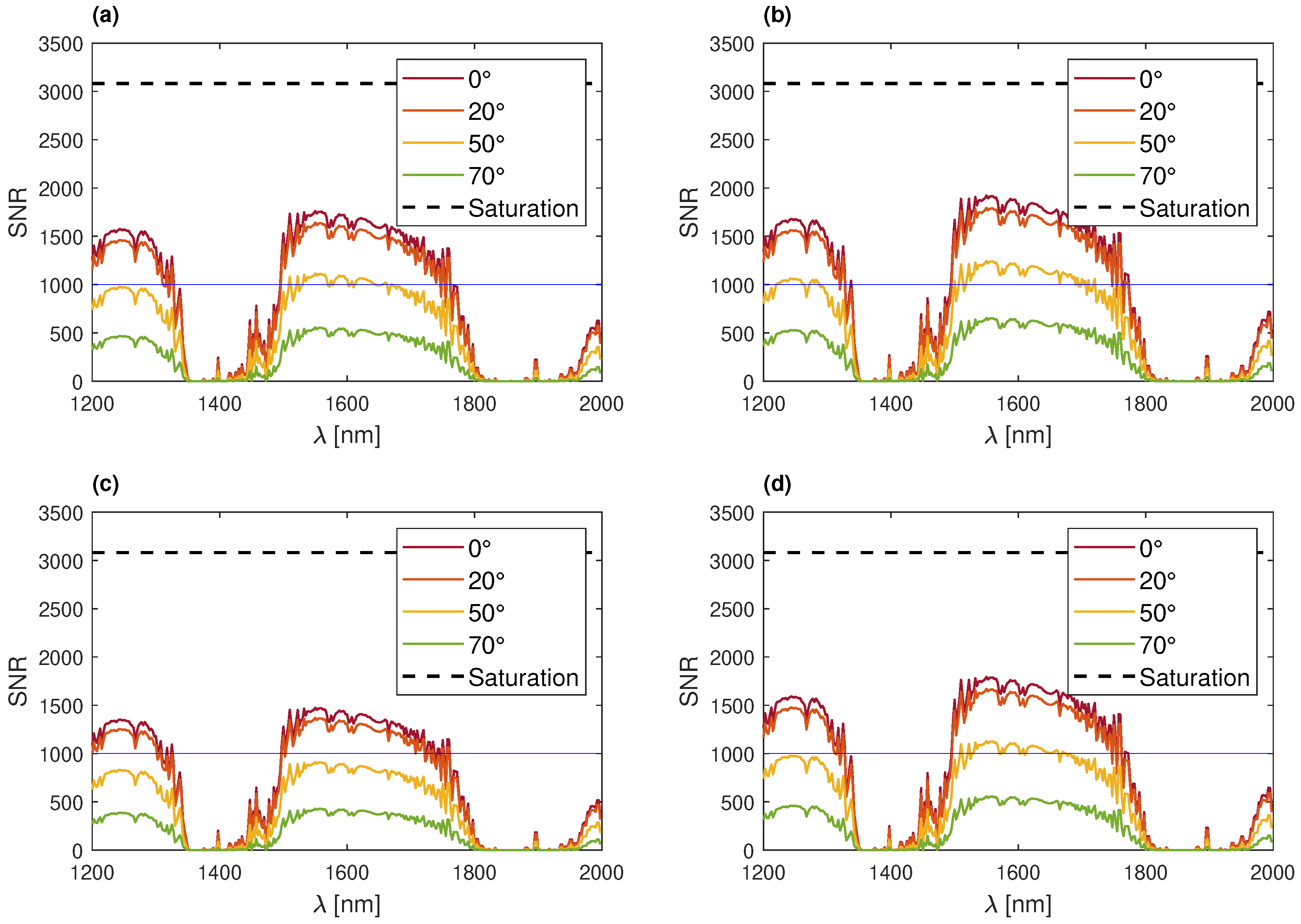
In two specific scenarios (observations of the ocean and when the Solar Zenith Angle exceeds 50°), the SNR does not reach 1000 regardless of the observed wavelength.

It is reasonable to infer that in these cases, measurement accuracies, as appraised by GHGRetrieval, are less optimal. Generally, a higher SNR correlates with improved accuracy expectations.

4.3. Evaluation of Uvsq-Sat NG’s GHG Concentration Retrieval (XCO₂ and XCH₄)

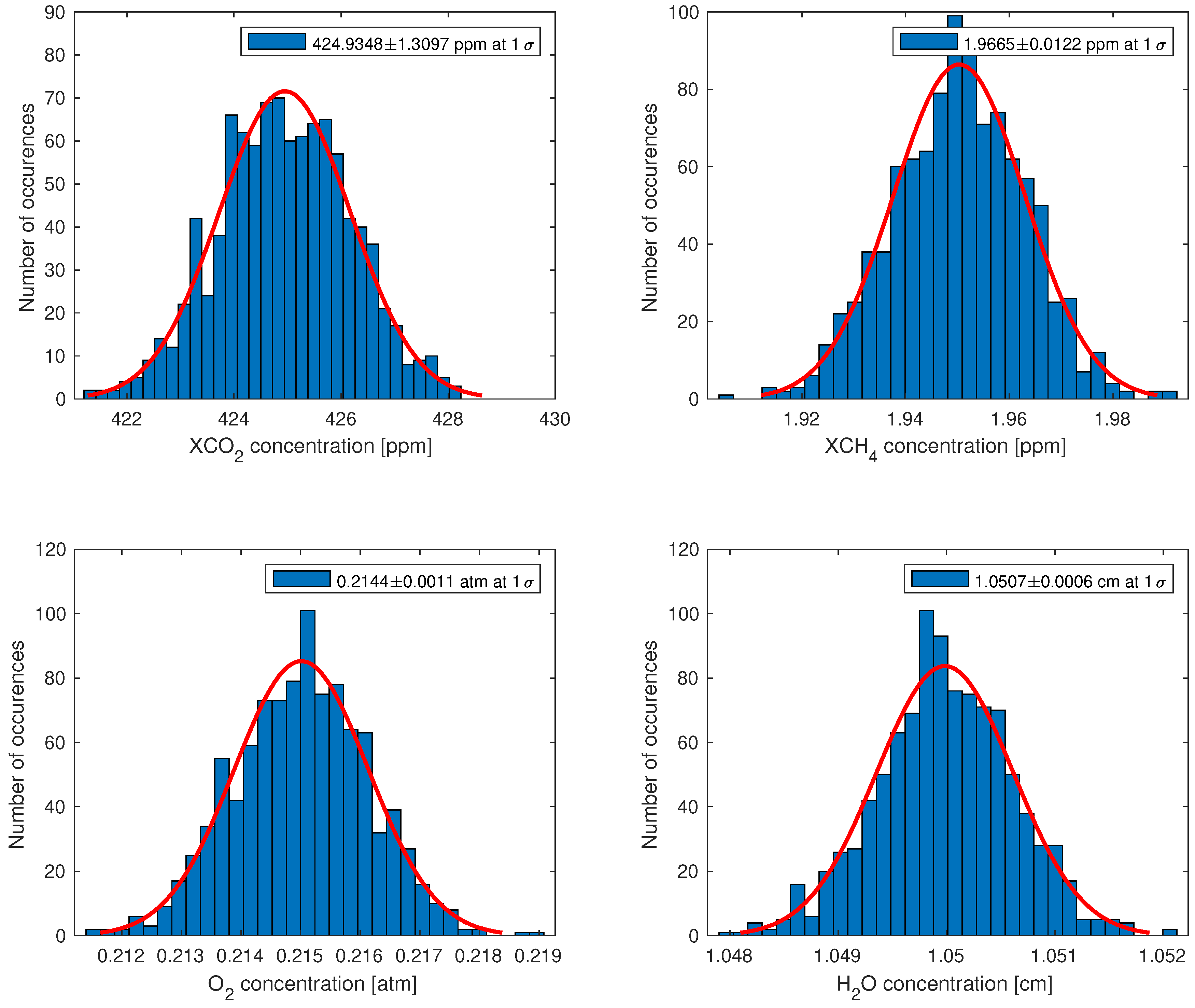
Figure 8 showcases the outcomes achieved for a possible observation scenario (pine forest targeted ‘Surface’, continental ‘Aerosols’, SZA of 20°) carried out by the Uvsq-Sat NG spectrometer (spectral resolution of 5 nm and SNR as a function of wavelength shown in Figure 6a). In this case, the uncertainties in retrieving the GHG concentrations are ±1.3 ppm for XCO₂ and ±12.2 ppb for XCH₄.

In total, 16 scenarios were studied, each involving a different ‘Aerosol’ type and a targeted ‘Surface’ with a SZA of 20°.

Table 3. Uncertainties of XCO₂ concentrations (1–Sigma) for several data retrievals based on different instrumental characteristics (spectral resolution and SNR) and for 16 scenarios with SZA of 20°.

Uvsq-Sat NG Spectrometer with a Spectral Resolution of 5 nm
	Surface	Pine Forest (a)	Deciduous Forest (b)	Ocean (c)	Homogeneous Snow (d)
Aerosols
Continental		1.3 ppm	0.9 ppm	234.5 ppm	0.7 ppm
Desert		1.7 ppm	0.8 ppm	225.8 ppm	0.6 ppm
Maritime		1.4 ppm	1.1 ppm	228.6 ppm	0.8 ppm
Urban		1.3 ppm	0.9 ppm	233.2 ppm	0.7 ppm
Future Uvsq-Sat NG-Type Spectrometer with a Spectral Resolution of 1 nm
	Surface	Pine forest (a)	Deciduous forest (b)	Ocean (c)	Homogeneous Snow (d)
Aerosols
Continental		0.5 ppm	0.4 ppm	77.6 ppm	0.3 ppm
Desert		0.5 ppm	0.3 ppm	82.8 ppm	0.3 ppm
Maritime		0.6 ppm	0.4 ppm	81.4 ppm	0.3 ppm
Urban		0.5 ppm	0.4 ppm	78.4 ppm	0.3 ppm

and

Table 4. Uncertainties of XCH₄ concentrations (1–Sigma) for several data retrievals based on different instrumental characteristics (spectral resolution and SNR) and for 16 scenarios with SZA of 20°.

Uvsq-Sat NG Spectrometer with a Spectral Resolution of 5 nm
	Surface	Pine Forest (a)	Deciduous Forest (b)	Ocean (c)	Homogeneous Snow (d)
Aerosols
Continental		12.2 ppb	10.2 ppb	735.6 ppb	7.8 ppb
Desert		10.5 ppb	8.5 ppb	710.8 ppb	7.0 ppb
Maritime		15.5 ppb	12.7 ppb	763.2 ppb	8.8 ppb
Urban		12.2 ppb	10.3 ppb	730.5 ppb	7.1 ppb
Future Uvsq-Sat NG-Type Spectrometer with a Spectral Resolution of 1 nm
	Surface	Pine forest (a)	Deciduous forest (b)	Ocean (c)	Homogeneous Snow (d)
Aerosols
Continental		4.9 ppb	3.7 ppb	194.1 ppb	2.5 ppb
Desert		4.4 ppb	3.2 ppb	184.8 ppb	2.4 ppb
Maritime		5.8 ppb	4.2 ppb	202.2 ppb	3.2 ppb
Urban		4.7 ppb	3.4 ppb	193.4 ppb	2.8 ppb

provide the findings related to the retrieval of the concentration of gases (XCO₂ and XCH₄) that could be observed with the Uvsq-Sat NG NIR spectrometer and for a future Uvsq-Sat NG-type spectrometer with a spectral resolution of 1 nm.

In addition, 16 other scenarios were studied with the same instrumental characteristics, each involving different SZAs and different ‘Aerosol’ types, with ‘Pine forest’ as the targeted ‘Surface’.

Table 5. Uncertainties of XCO₂ concentrations (1–Sigma) for several data retrievals based on different instrumental characteristics (spectral resolution and SNR) and for 16 scenarios with a pine forest-targeted ‘Surface’.

Uvsq-Sat NG Spectrometer with a Spectral Resolution of 5 nm
	Aerosols	Continental (a)	Desert (b)	Maritime (c)	Urban (d)
SZA
0°		1.2 ppm	1.0 ppm	1.3 ppm	1.1 ppm
20°		1.3 ppm	1.1 ppm	1.5 ppm	1.1 ppm
50°		2.0 ppm	1.7 ppm	2.4 ppm	2.0 ppm
70°		5.6 ppm	4.3 ppm	6.5 ppm	5.2 ppm
Future Uvsq-Sat NG-Type Spectrometer with a Spectral Resolution of 1 nm
	Aerosols	Continental (a)	Desert (b)	Maritime (c)	Urban (d)
SZA
0°		0.5 ppm	0.4 ppm	0.6 ppm	0.5 ppm
20°		0.5 ppm	0.5 ppm	0.6 ppm	0.5 ppm
50°		0.8 ppm	0.8 ppm	1.0 ppm	0.9 ppm
70°		2.2 ppm	1.7 ppm	2.9 ppm	2.2 ppm

and

Table 6. Uncertainties of XCH₄ concentrations (1–Sigma) for several data retrievals based on different instrumental characteristics (spectral resolution and SNR) and for 16 scenarios with a pine forest-targeted ‘Surface’.

Uvsq-Sat NG Spectrometer with a Spectral Resolution of 5 nm
	Aerosols	Continental (a)	Desert (b)	Maritime (c)	Urban (d)
SZA
0°		12.7 ppb	11.2 ppb	14.3 ppb	11.4 ppb
20°		13.1 ppb	12.5 ppb	15.2 ppb	12.8 ppb
50°		19.9 ppb	16.7 ppb	23.4 ppb	19.9 ppb
70°		41.0 ppb	37.8 ppb	53.1 ppb	39.8 ppb
Future Uvsq-Sat NG-Type Spectrometer with a Spectral Resolution of 1 nm
	Aerosols	Continental (a)	Desert (b)	Maritime (c)	Urban (d)
SZA
0°		4.2 ppb	3.8 ppb	5.0 ppb	4.1 ppb
20°		4.5 ppb	4.3 ppb	5.6 ppb	4.3 ppb
50°		7.3 ppb	5.8 ppb	8.9 ppb	6.6 ppb
70°		14.7 ppb	12.6 ppb	19.4 ppb	14.7 ppb

provide the results associated with these scenarios, which allow for the determination of the column average of carbon dioxide (XCO₂) and methane (XCH₄) in the atmosphere.

The obtained results demonstrate good assessments of the performances of the Uvsq-Sat NG satellite spectrometer. Indeed, the conducted simulations show that the retrieval of GHG concentrations (XCO₂ and XCH₄) is in good agreement with scientific requirements (Table 1) for a large number of scenarios. The scientific requirements for the Uvsq-Sat NG spectrometer were set at a 4 ppm uncertainty for XCO₂ measurements and 25 ppb for XCH₄ measurements. For all Uvsq-Sat NG instrumental parameters, none of the scenarios with an ocean-targeted ‘Surface’ meets the scientific requirements for retrieving GHG concentrations.

5. Discussions

SolAtmos was developed to assess the performance of the Uvsq-Sat NG spectrometer to monitor GHG in multiple scenarios. Among these scenarios, the most favorable observation case appears to be a snow-covered scene with desert aerosols with retrieval accuracy that can reach 0.6 ppm for the CO₂ column and 7.0 ppb for the CH₄. A study dating back to 2013 [36] investigates satellite observations of snow darkening in the Himalayas induced by desert dust. However, this scenario may not be the most likely in practice. In reality, maritime, continental, and urban aerosols are more common.

When considering a SZA of 20°, the primary influencing factor is the targeted surface type. Surfaces like homogeneous snow, which have significantly higher albedo compared to the ocean, reflect a substantial amount of incoming solar radiance. Polar observations may present the most favorable conditions for measurements with the highest accuracy.

Furthermore, Figure 5 examines the influence of different aerosol types and SZAs for a pine forest scene. In this context, variations in SZA have a more significant impact on incoming solar radiance than the type of aerosols. Based on the results, it appears that the impact of aerosols on the solar spectra remains relatively consistent across the entire 1200–2000 nm range. There does not seem to be a distinctive spectral signature of aerosols in the near-infrared region. It might be worth conducting a study to explore the possibility of identifying an aerosol signature in the near-infrared range.

All the simulations are considered under clear skies, which is the ideal observation case. However, obviously some observations could be contaminated by clouds. In this case, the data analysis is more complex and depends of the nature of the clouds. The Uvsq-Sat NG satellite is equipped with a camera that allows for scene observation and provides a criterion for the quality of the measurements made by the spectrometer. Additionally, we are considering using other satellite data (collocation) to verify the status of our observations. When the observed scenes are associated with very cloudy areas, the spectrometer cannot guarantee the observations.

According to the SolAtmos results, the most unfavorable observation cases occur above ocean scenes and for a SZA higher than 50°. In these two cases, the SolAtmos results show a lack of accuracy in retrieving GHG concentrations. Improving the accuracy in these scenarios can be achieved by increasing the SNR of the Uvsq-Sat NG spectrometer. Figure 9 illustrates the impact of integration time and SNR at a wavelength of 1600 nm on the radiance that can be measured in orbit. Radiance is determined using Equations (1) and (2), where the number of electrons is calculated based on a given SNR and integration time. Several scenarios are analyzed for different SNR values (1000, 1500 and 2000). Saturation as a function of integration time is determined using Equation (5), taking into account a maximum number of electrons of 17.5 million (full-well capacity).

According to Figure 9, it is possible to select an integration time based on the radiance at TOA to achieve an SNR of 2000 at 1600 nm without exceeding the saturation level. Figure 9 illustrates the possibility of choosing an appropriate integration time at a specific wavelength. For example, in the case of an ocean scene where the radiance at TOA is about 0.005 Wm⁻²sr⁻¹nm⁻¹, the integration time should be greater than 700 ms to achieve an SNR of 1500. However, this solution is not viable if the integration time remains constant throughout the Uvsq-Sat NG satellite orbit. In that scenario, above continental scenes, the signal exceeds the saturation level. When the integration time remains fixed, there may be a trade-off between high accuracy over continental scenes and high accuracy over oceans.

Another potential solution is to adapt the integration time based on the Uvsq-Sat NG satellite’s location, leveraging Global Navigation Satellite Systems (GNSSs) and Artificial Intelligence (AI). However, increasing the measurement time results in a decrease in the ground footprint. The Uvsq-Sat NG spectrometer’s spatial resolution is approximately 2 km, and the satellite’s speed is approximately 6 kilometers per second relative to the surface of the Earth. With an integration time of 700 ms, the ground footprint for nadir pointing is around 5 km. In this scenario, the identification of local GHG sources and sinks is made more difficult. Additionally, significantly increasing the integration time to enhance spectral SNR could potentially push the Uvsq-Sat NG CMOS sensor to saturation.

The most viable solution to consider is adding a glint pointing mode to the Uvsq-Sat NG satellite. Glint observations refer to a specific technique used in remote sensing and Earth observation satellite missions, particularly when observing oceans. Glint observations involve capturing the sunlight that is reflected off the surface of the water. This reflected sunlight creates a bright, shimmering effect on the water’s surface, which is known as ‘Sun glint’. The ‘Sun glint’ approach has been utilized by missions like GOSAT and OCO-2 to enhance signal strength over oceans [37,38]. The Uvsq-Sat NG mission will also harness the Sun glint on the ocean to enhance the signal received by its NIR spectrometer’s sensor in specific geographical areas. This approach is necessary because Sun glint does not occur above 60°N and below 60°S [39]. To validate this pointing mode using our SolAtmos end-to-end simulator with its three tools (IRIS, OptiSpectra, GHGRetrieval), it is necessary to employ a different radiative transfer code than the 6SV radiative transfer model, which can only simulate nadir pointing. The SCIATRAN radiative transfer model could be a suitable candidate for this purpose, but also to allow for the study of instruments with spectral resolutions less than 2.5 nm, like, for instance, a future Uvsq-Sat NG-type spectrometer with a spectral resolution of 1 nm.

Indeed, a spectrometer with a higher spectral resolution is of interest if we consider GHG requirements on the order of 1 ppm for CO₂ and 10 ppb for CH₄. For this future spectrometer, the 2.5 nm spectral resolution of the 6SV radiative code is insufficient. Typically, it is more advantageous to simulate radiance at a significantly higher spectral resolution than that of the spectrometer and subsequently convolve it with the spectrometer’s slit function. In this instance, the results we obtained lead to a loss of fine spectral details and less accurate determination of GHG concentrations. In future studies, we will integrate SCIATRAN (spectral resolution less than 0.2 nm on NIR) to enhance our tools.

When the satellite observes at SZAs exceeding 50°, there are limitations to the data quality due to reduced SNR of the Uvsq-Sat NG spectrometer and its spectral resolution of ∼5 nm. In such scenarios, it becomes challenging to observe GHG with an excellent accuracy. This is one of the reasons why we aim to develop, in the future, a new spectrometer similar to Uvsq-Sat NG with a spectral resolution of approximately 1 nm. Such a new spectrometer with a 1 nm spectral resolution is still suitable for scientific needs when observing over continental surfaces with different aerosol types, but only if the SZA remains below 50° (Table 5 and Table 6).

6. Conclusions

The SolAtmos end-to-end simulator, along with its tools, IRIS, OptiSpectra, and GHGRetrieval, was implemented to evaluate the capabilities of monitoring greenhouse gases, particularly carbon dioxide and methane, from a space-based instrument. This simulator is used to assess the scientific performance of the Uvsq-Sat NG mission. This simulator is implemented to be applicable to other observation missions as well. To be even more efficient, SolAtmos needs to fully integrate the SCIATRAN and DART radiative transfer models.

Thus, three new tools were developed. IRIS provides the spectral radiations at TOA to predict the quantities observed by the Uvsq-Sat NG spectrometer, while OptiSpectra determines the optimal observation parameters. GHGRetrieval is used to retrieve the concentrations of GHGs observed by the space instrument.

SolAtmos is used to verify the performances of the Uvsq-Sat NG mission mainly dedicated to GHG observations. The results, in turn, demonstrate that the Uvsq-Sat NG spectrometer is highly proficient in accurately observing carbon dioxide and methane concentrations. This high level of accuracy applies to a majority of observed scenes, which include different surface types such as pine forests, deciduous forests, and homogeneous snow, as well as different aerosol types like continental, desert, and maritime. The expected accuracy for each measurement above continental scenes with a SZA of less than 50° is 2.4 ppm for the carbon dioxide column and 23.4 ppb for the methane column, which perfectly meets Uvsq-Sat NG scientific requirements. However, it is important to note that the uncertainty in determining the concentrations of carbon dioxide and methane is higher when observing the oceans. This increased uncertainty over oceanic regions is a crucial factor to consider in the overall performance of the satellite’s observational capabilities. In this case, a Sun glint mode will be implemented in the framework of the Uvsq-Sat NG operations in orbit. It represents a specialized observational technique designed to enhance the satellite’s ability to accurately measure atmospheric gas concentrations, particularly carbon dioxide and methane, over oceanic regions.

These simulations demonstrate that a small satellite equipped with a low-resolution spectrometer can effectively measure GHGs with good accuracy. Multiple satellites of this kind in constellations enable the observation of greenhouse gases in near-real-time with excellent spatiotemporal resolution.

References

- Shearman, D.; Smith, J.W. The Climate Change Challenge and the Failure of Democracy; Bloomsbury Publishing: New York, NY, USA, 2007. [Google Scholar]
- Ripple, W.J.; Wolf, C.; Newsome, T.M.; Barnard, P.; Moomaw, W.R. World scientists’ warning of a climate emergency. BioScience 2020, 70, 8–100. [Google Scholar] [CrossRef]
- Javadinejad, S.; Dara, R.; Jafary, F. Investigation of the effect of climate change on heat waves. Resour. Environ. Inf. Eng. 2020, 2, 54–60. [Google Scholar] [CrossRef]
- Siddik, M.; Islam, M.; Zaman, A.; Hasan, M. Current status and correlation of fossil fuels consumption and greenhouse gas emissions. Int. J. Energy Environ. Econ 2021, 28, 103–119. [Google Scholar]
- Zemp, M.; Chao, Q.; Han Dolman, A.J.; Herold, M.; Krug, T.; Speich, S.; Suda, K.; Thorne, P.; Yu, W. GCOS 2022 Implementation Plan. In Global Climate Observing System GCOS; ESA Climate Office: Oxfordshire, UK, 2022; p. 85. [Google Scholar]
- Friedlingstein, P.; Jones, M.W.; O’sullivan, M.; Andrew, R.M.; Bakker, D.C.; Hauck, J.; Le Quéré, C.; Peters, G.P.; Peters, W.; Pongratz, J.; et al. Global carbon budget 2021. Earth Syst. Sci. Data 2022, 14, 1917–2005. [Google Scholar] [CrossRef]
- Saunois, M.; Stavert, A.R.; Poulter, B.; Bousquet, P.; Canadell, J.G.; Jackson, R.B.; Raymond, P.A.; Dlugokencky, E.J.; Houweling, S.; Patra, P.K.; et al. The global methane budget 2000–2017. Earth Syst. Sci. Data 2020, 12, 1561–1623. [Google Scholar] [CrossRef]
- Meftah, M.; Damé, L.; Keckhut, P.; Bekki, S.; Sarkissian, A.; Hauchecorne, A.; Bertran, E.; Carta, J.P.; Rogers, D.; Abbaki, S.; et al. UVSQ-SAT, a pathfinder cubesat mission for observing essential climate variables. Remote Sens. 2020, 12, 92. [Google Scholar] [CrossRef]
- Meftah, M.; Boust, F.; Keckhut, P.; Sarkissian, A.; Boutéraon, T.; Bekki, S.; Damé, L.; Galopeau, P.; Hauchecorne, A.; Dufour, C.; et al. Inspire-sat 7, a second cubesat to measure the earth’s energy budget and to probe the ionosphere. Remote Sens. 2022, 14, 186. [Google Scholar] [CrossRef]
- Meftah, M.; Clavier, C.; Sarkissian, A.; Hauchecorne, A.; Bekki, S.; Lefèvre, F.; Galopeau, P.; Dahoo, P.R.; Pazmino, A.; Vieau, A.J.; et al. Uvsq-Sat NG, a New CubeSat Pathfinder for Monitoring Earth Outgoing Energy and Greenhouse Gases. Remote Sens. 2023, 15, 4876. [Google Scholar] [CrossRef]
- Ciais, P.; Tan, J.; Wang, X.; Roedenbeck, C.; Chevallier, F.; Piao, S.L.; Moriarty, R.; Broquet, G.; Le Quéré, C.; Canadell, J.; et al. Five decades of northern land carbon uptake revealed by the interhemispheric CO2 gradient. Nature 2019, 568, 221–225. [Google Scholar] [CrossRef] [PubMed]
- Friedlingstein, P.; O’Sullivan, M.; Jones, M.; Andrew, R.; Hauck, J.; Olsen, A.; Peters, G.; Peters, W.; Pongratz, J.; Sitch, S.; et al. Global Carbon Budget 2020. Earth Syst. Sci. Data 2020, 12, 3269–3340. [Google Scholar] [CrossRef]
- Schneising, O.; Bergamaschi, P.; Bovensmann, H.; Buchwitz, M.; Burrows, J.P.; Deutscher, N.M.; Griffith, D.W.T.; Heymann, J.; Macatangay, R.; Messerschmidt, J.; et al. Atmospheric greenhouse gases retrieved from SCIAMACHY: Comparison to ground-based FTS measurements and model results. Atmos. Chem. Phys. 2012, 12, 1527–1540. [Google Scholar] [CrossRef]
- Kuze, A.; Suto, H.; Shiomi, K.; Kawakami, S.; Tanaka, M.; Ueda, Y.; Deguchi, A.; Yoshida, J.; Yamamoto, Y.; Kataoka, F.; et al. Update on GOSAT TANSO-FTS performance, operations, and data products after more than 6 years in space. Atmos. Meas. Tech. 2016, 9, 2445–2461. [Google Scholar] [CrossRef]
- Worden, J.R.; Doran, G.; Kulawik, S.; Eldering, A.; Crisp, D.; Frankenberg, C.; O’Dell, C.; Bowman, K. Evaluation and attribution of OCO-2 XCO2 uncertainties. Atmos. Meas. Tech. 2017, 10, 2759–2771. [Google Scholar] [CrossRef]
- Jervis, D.; McKeever, J.; Durak, B.O.; Sloan, J.J.; Gains, D.; Varon, D.J.; Ramier, A.; Strupler, M.; Tarrant, E. The GHGSat-D imaging spectrometer. Atmos. Meas. Tech. 2021, 14, 2127–2140. [Google Scholar] [CrossRef]
- Lorente, A.; Borsdorff, T.; Butz, A.; Hasekamp, O.; aan de Brugh, J.; Schneider, A.; Wu, L.; Hase, F.; Kivi, R.; Wunch, D.; et al. Methane retrieved from TROPOMI: Improvement of the data product and validation of the first 2 years of measurements. Atmos. Meas. Tech. 2021, 14, 665–684. [Google Scholar] [CrossRef]
- Meftah, M.; Sarkissian, A.; Keckhut, P.; Hauchecorne, A. The SOLAR-HRS New High-Resolution Solar Spectra for Disk-Integrated, Disk-Center, and Intermediate Cases. Remote Sens. 2023, 15, 3560. [Google Scholar] [CrossRef]
- Ehret, G.; Bousquet, P.; Pierangelo, C.; Alpers, M.; Millet, B.; Abshire, J.B.; Bovensmann, H.; Burrows, J.P.; Chevallier, F.; Ciais, P.; et al. MERLIN: A French-German space lidar mission dedicated to atmospheric methane. Remote Sens. 2017, 9, 1052. [Google Scholar] [CrossRef]
- Bovensmann, H.; Burrows, J.; Buchwitz, M.; Frerick, J.; Noel, S.; Rozanov, V.; Chance, K.; Goede, A. SCIAMACHY: Mission objectives and measurement modes. J. Atmos. Sci. 1999, 56, 127–150. [Google Scholar] [CrossRef]
- Schneising, O.; Heymann, J.; Buchwitz, M.; Reuter, M.; Bovensmann, H.; Burrows, J. Anthropogenic carbon dioxide source areas observed from space: Assessment of regional enhancements and trends. Atmos. Chem. Phys. 2013, 13, 2445–2454. [Google Scholar] [CrossRef]
- Vermote, E.F.; Tanré, D.; Deuze, J.L.; Herman, M.; Morcette, J.J. Second simulation of the satellite signal in the solar spectrum, 6S: An overview. IEEE Trans. Geosci. Remote. Sens. 1997, 35, 675–686. [Google Scholar] [CrossRef]
- Rozanov, V.; Rozanov, A.; Kokhanovsky, A.; Burrows, J. Radiative transfer through terrestrial atmosphere and ocean: Software package SCIATRAN. J. Quant. Spectrosc. Radiat. Transf. 2014, 133, 13–71. [Google Scholar] [CrossRef]
- Scott, N.A.; Chedin, A. A Fast Line-by-Line Method for Atmospheric Absorption Computations: The Automatized Atmospheric Absorption Atlas. J. Appl. Meteorol. Climatol. 1981, 20, 802–812. [Google Scholar] [CrossRef]
- Gastellu-Etchegorry, J.P.; Yin, T.; Lauret, N.; Cajgfinger, T.; Gregoire, T.; Grau, E.; Feret, J.B.; Lopes, M.; Guilleux, J.; Dedieu, G.; et al. Discrete anisotropic radiative transfer (DART 5) for modeling airborne and satellite spectroradiometer and LIDAR acquisitions of natural and urban landscapes. Remote Sens. 2015, 7, 1667–1701. [Google Scholar] [CrossRef]
- Clough, S.A.; Kneizys, F.X.; Rothman, L.S.; Gallery, W.O. Atmospheric Spectral Transmittance And Radiance: FASCOD1 B. In Proceedings of the Atmospheric Transmission, Washington, DC, USA, 21–22 April 1981; Fan, R.W., Ed.; International Society for Optics and Photonics, SPIE: Belligham, WA, USA, 1981; Volume 0277, pp. 152–167. [Google Scholar] [CrossRef]
- Berk, A.; Bernstein, L.; Anderson, G.; Acharya, P.; Robertson, D.; Chetwynd, J.; Adler-Golden, S. MODTRAN Cloud and Multiple Scattering Upgrades with Application to AVIRIS. Remote Sens. Environ. 1998, 65, 367–375. [Google Scholar] [CrossRef]
- Mayer, B.; Kylling, A. The libRadtran software package for radiative transfer calculations-description and examples of use. Atmos. Chem. Phys. 2005, 5, 1855–1877. [Google Scholar] [CrossRef]
- Vermote, E.; Tanré, D.; Deuzé, J.; Herman, M.; Morcrette, J.; Kotchenova, S. Second simulation of a satellite signal in the solar spectrum-vector (6SV). 6S User Guide Version 2006, 3, 1–55. [Google Scholar]
- Gordon, I.E.; Rothman, L.S.; Hargreaves, R.; Hashemi, R.; Karlovets, E.V.; Skinner, F.; Conway, E.K.; Hill, C.; Kochanov, R.V.; Tan, Y.; et al. The HITRAN2020 molecular spectroscopic database. J. Quant. Spectrosc. Radiat. Transf. 2022, 277, 107949. [Google Scholar]
- Wang, Y.; Gastellu-Etchegorry, J.P. DART: Improvement of thermal infrared radiative transfer modelling for simulating top of atmosphere radiance. Remote. Sens. Environ. 2020, 251, 112082. [Google Scholar] [CrossRef]
- Peacock, K.; Warren, J.W.; Darlington, E.H. The near-infrared spectrometer. Johns Hopkins Apl Tech. Dig. 1998, 19, 115. [Google Scholar]
- Zemax, L.L.C.; Kirkland, W.A. ZEMAX Optical Design Program: User’s Guide; University of California: San Diego, CA, USA, 2009. [Google Scholar]
- Ceccherini, S.; Ridolfi, M. Technical Note: Variance-covariance matrix and averaging kernels for the Levenberg-Marquardt solution of the retrieval of atmospheric vertical profiles. Atmos. Chem. Phys. 2010, 10, 3131–3139. [Google Scholar] [CrossRef]
- Bertaux, J.L.; Hauchecorne, A.; Lefèvre, F.; Bréon, F.M.; Blanot, L.; Jouglet, D.; Lafrique, P.; Akaev, P. The use of the 1.27 μm O2 absorption band for greenhouse gas monitoring from space and application to MicroCarb. Atmos. Meas. Tech. 2020, 13, 3329–3374. [Google Scholar] [CrossRef]
- Gautam, R.; Hsu, N.C.; Lau, W.K.M.; Yasunari, T.J. Satellite observations of desert dust-induced Himalayan snow darkening. Geophys. Res. Lett. 2013, 40, 988–993. [Google Scholar] [CrossRef]
- Zhou, M.; Dils, B.; Wang, P.; Detmers, R.; Yoshida, Y.; O’Dell, C.W.; Feist, D.G.; Velazco, V.A.; Schneider, M.; De Mazière, M. Validation of TANSO-FTS/GOSAT XCO2 and XCH4 glint mode retrievals using TCCON data from near-ocean sites. Atmos. Meas. Tech. 2016, 9, 1415–1430. [Google Scholar] [CrossRef]
- Wunch, D.; Wennberg, P.O.; Osterman, G.; Fisher, B.; Naylor, B.; Roehl, C.M.; O’Dell, C.; Mandrake, L.; Viatte, C.; Kiel, M.; et al. Comparisons of the Orbiting Carbon Observatory-2 (OCO-2) XCO2 measurements with TCCON. Atmos. Meas. Tech. 2017, 10, 2209–2238. [Google Scholar] [CrossRef]
- Lorente, A.; Borsdorff, T.; Martinez-Velarte, M.C.; Butz, A.; Hasekamp, O.P.; Wu, L.; Landgraf, J. Evaluation of the methane full-physics retrieval applied to TROPOMI ocean sun glint measurements. Atmos. Meas. Tech. 2022, 15, 6585–6603. [Google Scholar] [CrossRef]
Figure 1.
Description of the SolAtmos end-to-end simulator.
Figure 2.
Illustration of an optical layout of the Uvsq-Sat NG space-based spectrometer.
Figure 3.
The IRIS tool, with the currently available modules highlighted in yellow. The SCIATRAN radiative transfer code can be implemented as an alternative with higher spectral resolution and better atmospheric tunability compared to Py6S. These upgrades are designed to meet new requirements of the GHGRetrieval tool (high resolution), which includes the ‘Levenberg–Marquardt GES and O2 retrieval’ and ‘Retrieval GES and O2’ modules.
Figure 4.
TOA radiance in 16 scenarios: variations in ‘Aerosol’ types and targeted ‘Surface’ at SZA of 20°—(a) Pine forest, (b) Deciduous forest, (c) Ocean, and (d) Homogeneous snow.
Figure 5.
TOA radiance in 16 scenarios studied for different SZA and ‘Aerosol’ types—(a) Continental, (b) Desert, (c) Maritime, and (d) Urban aerosols.
Figure 6.
SNR of the spectrometer in 16 scenarios—variations in ‘Aerosol’ types and targeted ‘Surface’ at SZA of 20°—(a) Pine forest, (b) Deciduous forest, (c) Ocean, and (d) Homogeneous snow. The blue line represents an arbitrary SNR value of 1000.
Figure 7.
SNR of the spectrometer in 16 scenarios studied for different SZA and ‘Aerosol’ types—(a) Continental, (b) Desert, (c) Maritime, and (d) Urban aerosols. The blue line represents an arbitrary SNR value of 1000.
Figure 8.
Retrieval of the concentration of gases that could be observed via the Uvsq-Sat NG NIR spectrometer (spectral resolution of 5 nm and SNR dependent on wavelength) for a specific observation scenario (targeted ‘Surface’—pine forest, ‘Aerosols’—continental, SZA of 20°). For obtaining the histograms, we find a mean square deviation equal to the uncertainty determined by the Levenberg–Marquardt algorithm.
Figure 9.
Evolution of radiance at 1600 nm as a function of integration time for different SNR values.