
Studying the Internal Wave Generation Mechanism in the Northern South China Sea Using Numerical Simulation, Synthetic Aperture Radar, and In Situ Measurements

Abstract
:
1. Introduction
2. Data and Methods
2.1. Workflow Description
2.2. Types of Tides
2.3. Study Area and Data
2.4. Numerical Simulation
3. Results
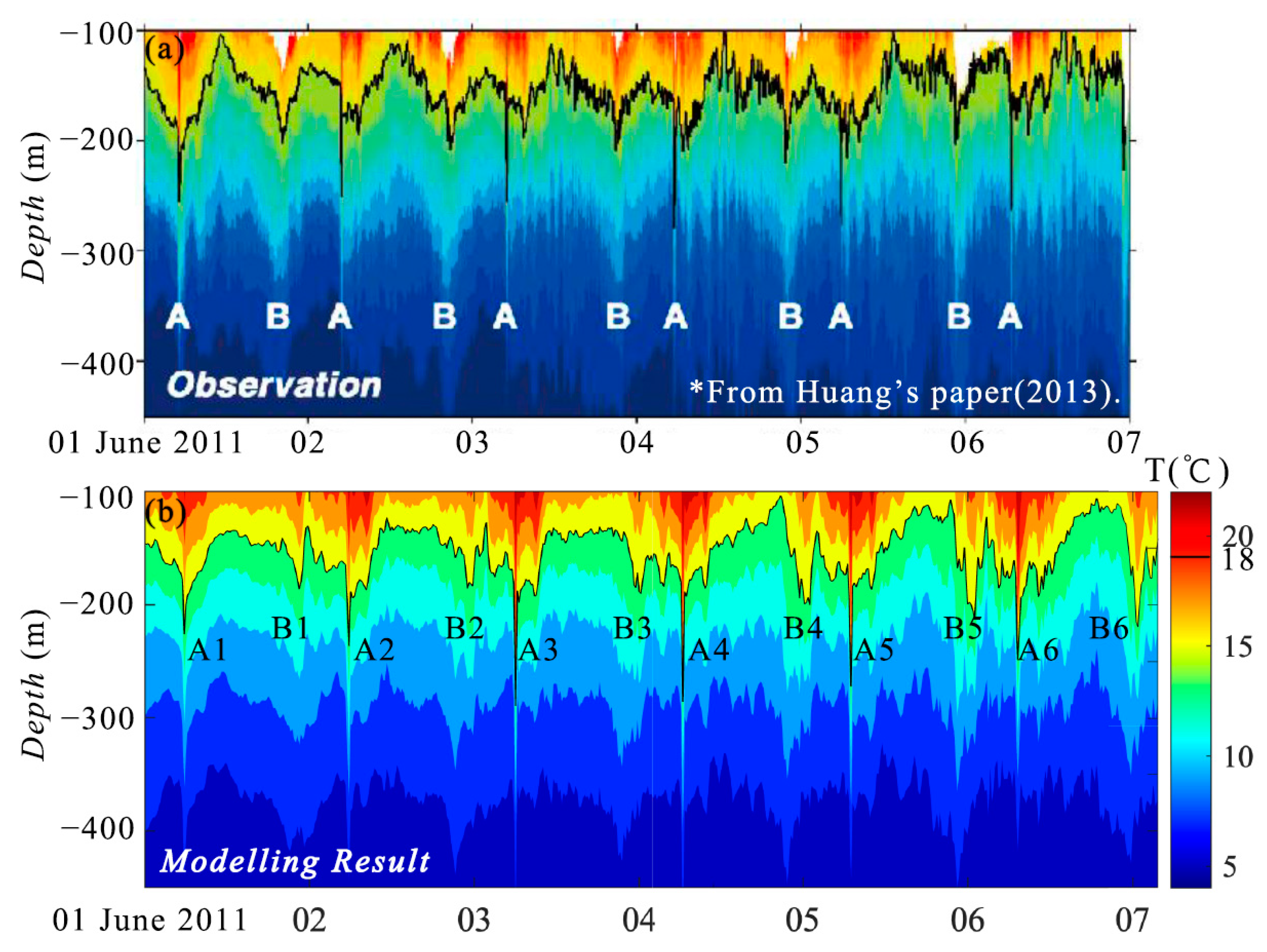
3.1. Model Validation
3.2. Generation Time and Location
3.3. Diurnal-Tide-Dominated Phase (DTP)
3.4. Transition Tide Phase (TTP)
3.5. Semidiurnal-Tide-Dominated Phase (STP)
4. Discussion
4.1. Diurnal-Tide-Dominated Phase (DTP)
4.2. Transition Tide Phase (TTP)
4.3. Semidiurnal-Tide-Dominated Phase (STP)
5. Conclusions
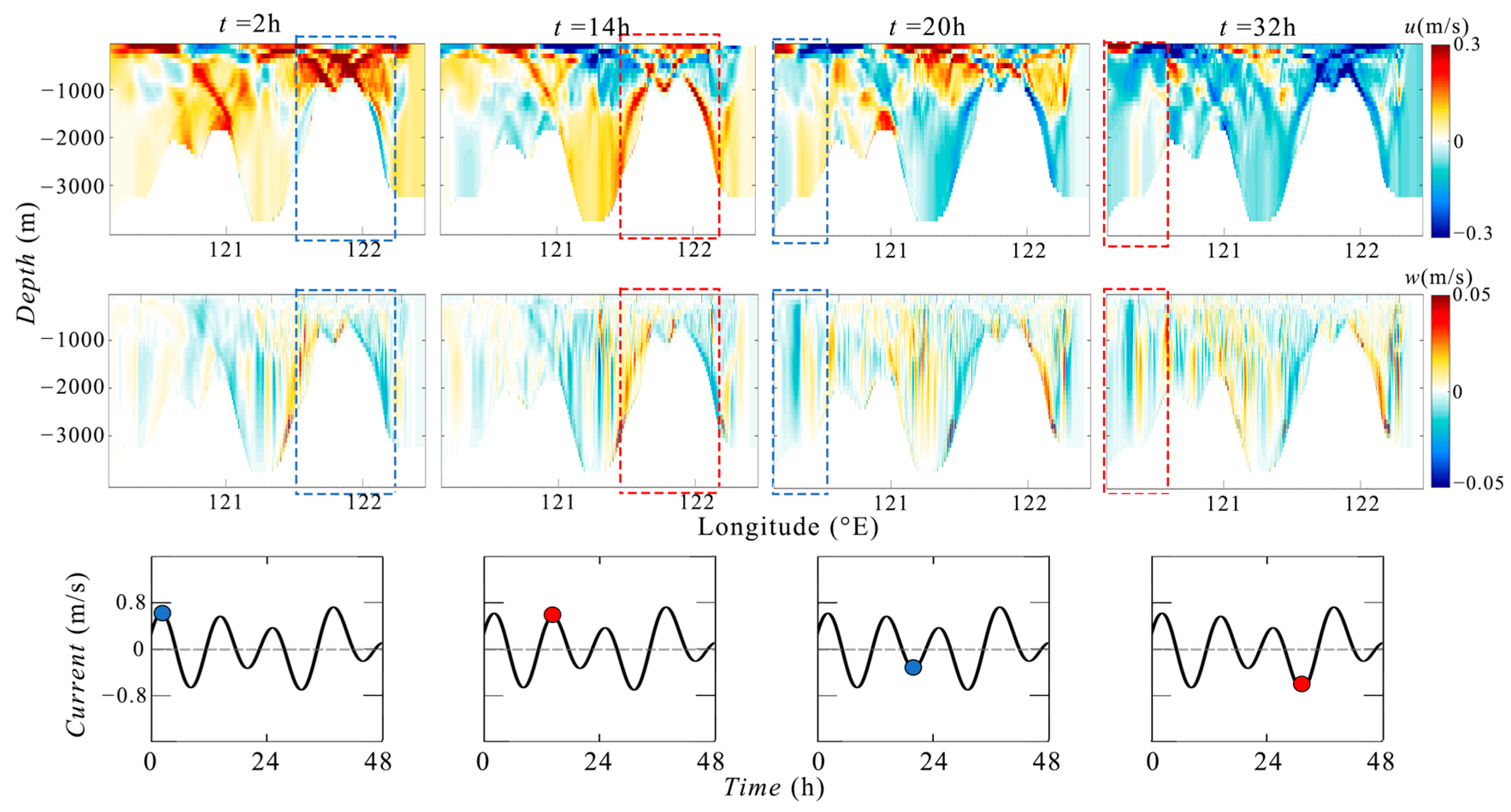
- Barotropic tidal currents oscillating relative to submarine ridges generate internal lee waves. These lee waves are always formed on the eastern side of the ridges and start propagating westward at the peak of the eastward tidal current, presenting as a concave surge. The strength of the surge is directly proportional to the intensity of the tidal current and inversely proportional to the depth of water over the ridge’s crest. The lee wave mechanism is effective for both the eastern and western ridges, but their intensities are different. For the same tidal current strength, the lee waves at the eastern ridge are significantly stronger than those at the western ridge. A lee wave must reach a certain intensity to have the potential to evolve into an internal solitary wave. Therefore, during the diurnal tidal peak moments of the DTP, diurnal tidal peak moments of the TTP, and semidiurnal tidal peak moments of the STP, the lee waves generated at the eastern ridge can eventually develop into Type A internal solitary waves.
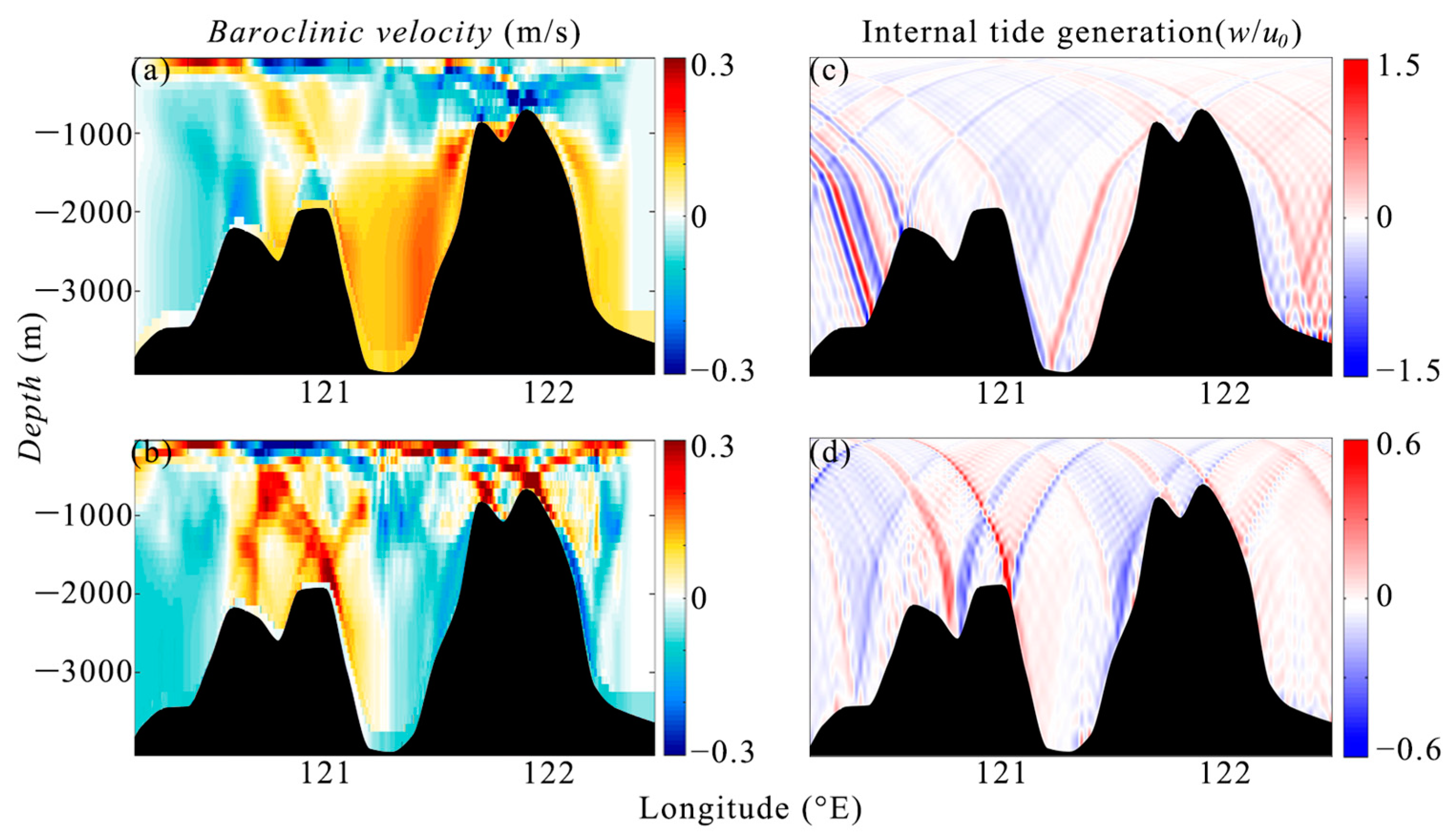
- Internal tides generated at the eastern ridge can propagate along ray paths and strike the top of the western ridge, with the propagation time coinciding with a semidiurnal tidal cycle. This synchronicity can lead to resonance between the lee waves generated at the western ridge and the rays emanating from the eastern ridge during the previous semidiurnal tidal cycle. Clearly, this resonance effect only occurs when the semidiurnal tidal component is strong. Thus, resonance occurs during the TTP and STP, but not during the DTP.
- During the DTP, in the absence of resonance, even under strong tidal currents, the lee waves at the western ridge remain relatively weak, resulting in weaker Type B internal solitary waves.
- In contrast, during the TTP and STP, the resonance effect strengthens the lee waves at the western ridge. This leads to the development of stronger Type B internal solitary waves during the TTP, and even Type A waves during the STP.
- As a result, during the DTP, weaker Type A and Type B waves alternate daily; during the TTP, stronger daily alternations of Type A and Type B waves occur; and in the STP, two weaker Type A waves are observed each day.
Author Contributions
Funding
Data Availability Statement
Acknowledgments
Conflicts of Interest
References
- Alford, M.H.; Peacock, T.; MacKinnon, J.A.; Nash, J.D.; Buijsman, M.C.; Centurioni, L.R.; Chao, S.-Y.; Chang, M.-H.; Farmer, D.M.; Fringer, O.B.; et al. The Formation and Fate of Internal Waves in the South China Sea. Nature 2015, 521, 65–69. [Google Scholar] [CrossRef]
- Li, Q.; Cao, S.; Luo, Y.; Zhang, K.; Yang, F. Basis Functions for Shallow-Water Temperature Profiles Based on the Internal-Wave Eigenmodes. Acta Oceanol. Sin. 2023, 42, 56–64. [Google Scholar] [CrossRef]
- Fu, L.-L.; Holt, B. Internal Waves in the Gulf of California: Observations from a Spaceborne Radar. J. Geophys. Res. Ocean. 1984, 89, 2053–2060. [Google Scholar] [CrossRef]
- Meunier, T.; Le Boyer, A.; Molodstov, S.; Bower, A.; Furey, H.; Robbins, P. Internal Wave Activity in the Deep Gulf of Mexico. Front. Mar. Sci. 2023, 10, 1285303. [Google Scholar] [CrossRef]
- Roustan, J.; Bordois, L.; Dumas, F.; Auclair, F.; Carton, X. In Situ Observations of the Small-scale Dynamics at Camarinal Sill—Strait of Gibraltar. J. Geophys. Res. Ocean. 2023, 128, e2023JC019738. [Google Scholar] [CrossRef]
- Brandt, P.; Rubino, A.; Alpers, W.; Backhaus, J.O. Internal Waves in the Strait of Messina Studied by a Numerical Model and Synthetic Aperture Radar Images from the ERS 1/2 Satellites. J. Phys. Oceanogr. 1997, 27, 648–663. [Google Scholar] [CrossRef]
- Fourniotis, N.T. Effect of Internal Waves on the Hydrodynamics of a Mediterranean Sea Strait. J. Mar. Sci. Eng. 2024, 12, 532. [Google Scholar] [CrossRef]
- Xie, J.; Du, H.; Gong, Y.; Niu, J.; He, Y.; Chen, Z.; Liu, G.; Liu, L.; Zhang, L.; Cai, S. The Role of Seasonal Circulation in the Variability of Dynamic Parameters of Internal Solitary Waves in the Sulu Sea. Prog. Oceanogr. 2023, 217, 103100. [Google Scholar] [CrossRef]
- Zeng, K.; Alpers, W. Generation of Internal Solitary Waves in the Sulu Sea and Their Refraction by Bottom Topography Studied by ERS SAR Imagery and a Numerical Model. Int. J. Remote Sens. 2004, 25, 1277–1281. [Google Scholar] [CrossRef]
- Sun, L.; Zhang, J.; Meng, J. A Study of the Spatial-Temporal Distribution and Propagation Characteristics of Internal Waves in the Andaman Sea Using MODIS. Acta Oceanol. Sin. 2019, 38, 121–128. [Google Scholar] [CrossRef]
- Osborne, A.; Burch, T. Internal Solitons in the Andaman Sea. Science 1980, 208, 451–460. [Google Scholar] [CrossRef]
- Fer, I.; Koenig, Z.; Kozlov, I.E.; Ostrowski, M.; Rippeth, T.P.; Padman, L.; Bosse, A.; Kolås, E. Tidally Forced Lee Waves Drive Turbulent Mixing along the Arctic Ocean Margins. Geophys. Res. Lett. 2020, 47, e2020GL088083. [Google Scholar] [CrossRef]
- Serebryany, A.; Khimchenko, E.; Popov, O.; Denisov, D.; Kenigsberger, G. Internal Waves Study on a Narrow Steep Shelf of the Black Sea Using the Spatial Antenna of Line Temperature Sensors. J. Mar. Sci. Eng. 2020, 8, 833. [Google Scholar] [CrossRef]
- Silvestrova, K.; Myslenkov, S.; Puzina, O.; Mizyuk, A.; Bykhalova, O. Water Structure in the Utrish Nature Reserve (Black Sea) during 2020–2021 According to Thermistor Chain Data. J. Mar. Sci. Eng. 2023, 11, 887. [Google Scholar] [CrossRef]
- Jackson, C.R. Atlas of Internal Solitary Waves—February 2004. Available online: https://www.internalwaveatlas.com/ (accessed on 18 March 2024).
- Wang, T.; Huang, X.; Zhao, W.; Zheng, S.; Yang, Y.; Tian, J. Internal Solitary Wave Activities near the Indonesian Submarine Wreck Site Inferred from Satellite Images. J. Mar. Sci. Eng. 2022, 10, 197. [Google Scholar] [CrossRef]
- Loder, J.W.; Brickman, D.; Horne, E.P.W. Detailed Structure of Currents and Hydrography on the Northern Side of Georges Bank. J. Geophys. Res. Ocean. 1992, 97, 14331–14351. [Google Scholar] [CrossRef]
- Lamb, K.G. Numerical Experiments of Internal Wave Generation by Strong Tidal Flow across a Finite Amplitude Bank Edge. J. Geophys. Res. Ocean. 1994, 99, 843–864. [Google Scholar] [CrossRef]
- Katavouta, A.; Thompson, K.R.; Lu, Y.; Loder, J.W. Interaction between the Tidal and Seasonal Variability of the Gulf of Maine and Scotian Shelf Region. J. Phys. Oceanogr. 2016, 46, 3279–3298. [Google Scholar] [CrossRef]
- Gao, J.; Ji, C.; Liu, Y.; Gaidai, O.; Ma, X.; Liu, Z. Numerical Study on Transient Harbor Oscillations Induced by Solitary Waves. Ocean Eng. 2016, 126, 467–480. [Google Scholar] [CrossRef]
- Gao, J.; Ma, X.; Dong, G.; Zang, J.; Ma, Y.; Zhou, L. Effects of Offshore Fringing Reefs on the Transient Harbor Resonance Excited by Solitary Waves. Ocean Eng. 2019, 190, 106422. [Google Scholar] [CrossRef]
- Gao, J.; Ma, X.; Chen, H.; Zang, J.; Dong, G. On Hydrodynamic Characteristics of Transient Harbor Resonance Excited by Double Solitary Waves. Ocean Eng. 2021, 219, 108345. [Google Scholar] [CrossRef]
- Huang, X.; Chen, Z.; Zhao, W.; Zhang, Z.; Zhou, C.; Yang, Q.; Tian, J. An Extreme Internal Solitary Wave Event Observed in the Northern South China Sea. Sci. Rep. 2016, 6, 30041. [Google Scholar] [CrossRef] [PubMed]
- Osborne, A.; Burch, T.; Scarlet, R. The Influence of Internal Waves on Deep-Water Drilling. J. Pet. Technol. 1978, 30, 1497–1504. [Google Scholar] [CrossRef]
- Cheng, S.; Yu, Y.; Li, Z.; Huang, Z.; Yang, Z.; Zhang, X.; Cui, Y.; Wu, J.; Liu, X.; Yu, J. The Influence of Internal Solitary Wave on Semi-Submersible Platform System Including Mooring Line Failure. Ocean Eng. 2022, 258, 111604. [Google Scholar] [CrossRef]
- Litter, A.D. Internal Waves: Their Influence Upon Naval Operations; ASW Sonar Technology Report; Defense Technical Information Center: Fort Belvoir, VA, USA, 1996.
- Wang, C.; Wei, D.; Guanghua, L.; Peng, D.; Sen, Z.; Zhuoyue, L.; Xiaopeng, C.; Haibao, H. Numerical Simulation of Influence of Ocean Internal Waves on Hydrodynamic Characteristics of Underwater Vehicles. Chin. Ship Res. 2022, 17, 102–111. [Google Scholar]
- Du, T.; Tseng, Y.; Yan, X. Impacts of Tidal Currents and Kuroshio Intrusion on the Generation of Nonlinear Internal Waves in Luzon Strait. J. Geophys. Res. Ocean. 2008, 113, C08015. [Google Scholar] [CrossRef]
- Hsu, M.-K.; Liu, A.K. Nonlinear Internal Waves in the South China Sea. Can. J. Remote Sens. 2000, 26, 72–81. [Google Scholar] [CrossRef]
- Zhao, Z.; Klemas, V.; Zheng, Q.; Yan, X. Remote Sensing Evidence for Baroclinic Tide Origin of Internal Solitary Waves in the Northeastern South China Sea. Geophys. Res. Lett. 2004, 31, L06302. [Google Scholar] [CrossRef]
- Jackson, C.R. An Empirical Model for Estimating the Geographic Location of Nonlinear Internal Solitary Waves. J. Atmos. Ocean. Technol. 2009, 26, 2243–2255. [Google Scholar] [CrossRef]
- Ebbesmeyer, C.; Coomes, C.A.; Hamilton, R.; Kurrus, K.A.; Sullivan, T.C.; Salem, B.L.; Romea, R.D.; Bauer, R.J. New Observations on Internal Waves (Solitons) in the South China Sea Using an Acoustic Doppler Current Profiler. Mar. Technol. Soc. 91 Proc. 1991, 165–175. [Google Scholar]
- Gong, Q.; Chen, L.; Diao, Y.; Xiong, X.; Sun, J.; Lv, X. On the Identification of Internal Solitary Waves from Moored Observations in the Northern South China Sea. Sci. Rep. 2023, 13, 3133. [Google Scholar] [CrossRef]
- Zang, Z.; Zhang, Y.; Chen, T.; Xie, B.; Zou, X.; Li, Z. A Numerical Simulation of Internal Wave Propagation on a Continental Slope and Its Influence on Sediment Transport. J. Mar. Sci. Eng. 2023, 11, 517. [Google Scholar] [CrossRef]
- Ponte, A.L.; Cornuelle, B.D. Coastal Numerical Modelling of Tides: Sensitivity to Domain Size and Remotely Generated Internal Tide. Ocean Model. 2013, 62, 17–26. [Google Scholar] [CrossRef]
- Simmons, H.; Chang, M.-H.; Chang, Y.-T.; Chao, S.-Y.; Fringer, O.; Jackson, C.R.; Ko, D.S. Modeling and Prediction of Internal Waves in the South China Sea. Oceanography 2011, 24, 88–99. [Google Scholar] [CrossRef]
- Lai, Z.; Jin, G.; Huang, Y.; Chen, H.; Shang, X.; Xiong, X. The Generation of Nonlinear Internal Waves in the South China Sea: A Three-dimensional, Nonhydrostatic Numerical Study. J. Geophys. Res. Ocean. 2019, 124, 8949–8968. [Google Scholar] [CrossRef]
- Zeng, K.; Huang, Z.; He, M. A Propagation Model for Internal Waves in South China Sea Based on Fast Marching Method. Trans. Oceanol. Limnol. 2019, 6, 23–33. [Google Scholar] [CrossRef]
- Ramp, S.R.; Tang, T.Y.; Duda, T.F.; Lynch, J.F.; Liu, A.K.; Chiu, C.-S.; Bahr, F.L.; Kim, H.-R.; Yang, Y.-J. Internal Solitons in the Northeastern South China Sea. Part I: Sources and Deep Water Propagation. IEEE J. Ocean. Eng. 2004, 29, 1157–1181. [Google Scholar] [CrossRef]
- Alford, M.H.; Lien, R.-C.; Simmons, H.; Klymak, J.; Ramp, S.; Yang, Y.J.; Tang, D.; Chang, M.-H. Speed and Evolution of Nonlinear Internal Waves Transiting the South China Sea. J. Phys. Oceanogr. 2010, 40, 1338–1355. [Google Scholar] [CrossRef]
- Sinnett, G.; Ramp, S.R.; Yang, Y.J.; Chang, M.-H.; Jan, S.; Davis, K.A. Large-Amplitude Internal Wave Transformation into Shallow Water. J. Phys. Oceanogr. 2022, 52, 2539–2554. [Google Scholar] [CrossRef]
- Buijsman, M.C.; Klymak, J.M.; Legg, S.; Alford, M.H.; Farmer, D.; MacKinnon, J.A.; Nash, J.D.; Park, J.-H.; Pickering, A.; Simmons, H. Three-Dimensional Double-Ridge Internal Tide Resonance in Luzon Strait. J. Phys. Oceanogr. 2014, 44, 850–869. [Google Scholar] [CrossRef]
- Buijsman, M.C.; Legg, S.; Klymak, J. Double-Ridge Internal Tide Interference and Its Effect on Dissipation in Luzon Strait. J. Phys. Oceanogr. 2012, 42, 1337–1356. [Google Scholar] [CrossRef]
- Farmer, D.; Li, Q.; Park, J. Internal Wave Observations in the South China Sea: The Role of Rotation and Non-linearity. Atmos.-Ocean 2009, 47, 267–280. [Google Scholar] [CrossRef]
- Echeverri, P.; Peacock, T. Internal Tide Generation by Arbitrary Two-Dimensional Topography. J. Fluid Mech. 2010, 659, 247–266. [Google Scholar] [CrossRef]
- Buijsman, M.; McWilliams, J.; Jackson, C. East-west Asymmetry in Nonlinear Internal Waves from Luzon Strait. J. Geophys. Res. Ocean. 2010, 115, C10057. [Google Scholar] [CrossRef]
- Buijsman, M.; Kanarska, Y.; McWilliams, J. On the Generation and Evolution of Nonlinear Internal Waves in the South China Sea. J. Geophys. Res. Ocean. 2010, 115, C02012. [Google Scholar] [CrossRef]
- Shaw, P.; Ko, D.S.; Chao, S. Internal Solitary Waves Induced by Flow over a Ridge: With Applications to the Northern South China Sea. J. Geophys. Res. Ocean. 2009, 114, C02019. [Google Scholar] [CrossRef]
- Zhao, Z.; Alford, M.H. Source and Propagation of Internal Solitary Waves in the Northeastern South China Sea. J. Geophys. Res. Ocean. 2006, 111, C11012. [Google Scholar] [CrossRef]
- Zhang, Z.; Fringer, O.; Ramp, S. Three-dimensional, Nonhydrostatic Numerical Simulation of Nonlinear Internal Wave Generation and Propagation in the South China Sea. J. Geophys. Res. Ocean. 2011, 116, C05022. [Google Scholar] [CrossRef]
- Vlasenko, V.; Guo, C.; Stashchuk, N. On the Mechanism of A-Type and B-Type Internal Solitary Wave Generation in the Northern South China Sea. Deep Sea Res. Part I Oceanogr. Res. Pap. 2012, 69, 100–112. [Google Scholar] [CrossRef]
- Chen, Y.; Shan Ko, D.; Shaw, P. The Generation and Propagation of Internal Solitary Waves in the South China Sea. J. Geophys. Res. Ocean. 2013, 118, 6578–6589. [Google Scholar] [CrossRef]
- Li, Q. Numerical Assessment of Factors Affecting Nonlinear Internal Waves in the South China Sea. Prog. Oceanogr. 2014, 121, 24–43. [Google Scholar] [CrossRef]
- Zeng, Z.; Chen, X.; Yuan, C.; Tang, S.; Chi, L. A Numerical Study of Generation and Propagation of Type-a and Type-b Internal Solitary Waves in the Northern South China Sea. Acta Oceanol. Sin. 2019, 38, 20–30. [Google Scholar] [CrossRef]
- Beardsley, R.C.; Duda, T.F.; Lynch, J.F.; Irish, J.D.; Ramp, S.R.; Chiu, C.-S.; Tang, T.Y.; Yang, Y.-J.; Fang, G. Barotropic Tide in the Northeast South China Sea. IEEE J. Ocean. Eng. 2004, 29, 1075–1086. [Google Scholar] [CrossRef]
- Huang, X. Study on the Spatial Distribution and Time Variation Characteristics of Solitary Waves in the South China Sea; Ocean University of China: Qingdao, China, 2013. [Google Scholar]
- Ramp, S.; Yang, Y.; Bahr, F. Characterizing the Nonlinear Internal Wave Climate in the Northeastern South China Sea. Nonlinear Process. Geophys. 2010, 17, 481–498. [Google Scholar] [CrossRef]
- Marshall, J.; Adcroft, A.; Hill, C.; Perelman, L.; Heisey, C. A Finite-volume, Incompressible Navier Stokes Model for Studies of the Ocean on Parallel Computers. J. Geophys. Res. Ocean. 1997, 102, 5753–5766. [Google Scholar] [CrossRef]
- Alpers, W. Theory of Radar Imaging of Internal Waves. Nature 1985, 314, 245–247. [Google Scholar] [CrossRef]
- Alpers, W.R.; Ross, D.B.; Rufenach, C.L. On the Detectability of Ocean Surface Waves by Real and Synthetic Aperture Radar. J. Geophys. Res. Ocean. 1981, 86, 6481–6498. [Google Scholar] [CrossRef]
- Guo, C.; Vlasenko, V.; Alpers, W.; Stashchuk, N.; Chen, X. Evidence of Short Internal Waves Trailing Strong Internal Solitary Waves in the Northern South China Sea from Synthetic Aperture Radar Observations. Remote Sens. Environ. 2012, 124, 542–550. [Google Scholar] [CrossRef]
- Zheng, Q.; Susanto, R.D.; Ho, C.; Song, Y.T.; Xu, Q. Statistical and Dynamical Analyses of Generation Mechanisms of Solitary Internal Waves in the Northern South China Sea. J. Geophys. Res. Ocean. 2007, 112, C03021. [Google Scholar] [CrossRef]
- Fang, X.; Du, T. Fundamentals of Oceanic Internal Waves and Internal Waves in the China Seas; Ocean University China Press: Qingdao, China, 2005; pp. 71–73. [Google Scholar]
- Egbert, G.D.; Erofeeva, S.Y. Efficient Inverse Modeling of Barotropic Ocean Tides. J. Atmos. Ocean. Technol. 2002, 19, 183–204. [Google Scholar] [CrossRef]
- Guo, C.; Chen, X.; Vlasenko, V.; Stashchuk, N. Numerical Investigation of Internal Solitary Waves from the Luzon Strait: Generation Process, Mechanism and Three-Dimensional Effects. Ocean Model. 2011, 38, 203–216. [Google Scholar] [CrossRef]
- Gong, Y.; Chen, X.; Xu, J.; Xie, J.; Chen, Z.; He, Y.; Cai, S. An Internal Solitary Wave Forecasting Model in the Northern South China Sea (ISWFM-NSCS). Geosci. Model Dev. Discuss. 2023, 16, 2851–2871. [Google Scholar] [CrossRef]
- Maxworthy, T. A Note on the Internal Solitary Waves Produced by Tidal Flow over a Three-dimensional Ridge. J. Geophys. Res. Ocean. 1979, 84, 338–346. [Google Scholar] [CrossRef]
- Jan, S.; Lien, R.-C.; Ting, C.-H. Numerical Study of Baroclinic Tides in Luzon Strait. J. Oceanogr. 2008, 64, 789–802. [Google Scholar] [CrossRef]
- Echeverri, P.; Yokossi, T.; Balmforth, N.; Peacock, T. Tidally Generated Internal-Wave Attractors between Double Ridges. J. Fluid Mech. 2011, 669, 354–374. [Google Scholar] [CrossRef]
- Echeverri, P.; Flynn, M.; Winters, K.B.; Peacock, T. Low-Mode Internal Tide Generation by Topography: An Experimental and Numerical Investigation. J. Fluid Mech. 2009, 636, 91–108. [Google Scholar] [CrossRef]
- Jackson, C.R.; Da Silva, J.C.; Jeans, G. The Generation of Nonlinear Internal Waves. Oceanography 2012, 25, 108–123. [Google Scholar] [CrossRef]
- Alford, M.H.; MacKinnon, J.A.; Nash, J.D.; Simmons, H.; Pickering, A.; Klymak, J.M.; Pinkel, R.; Sun, O.; Rainville, L.; Musgrave, R. Energy Flux and Dissipation in Luzon Strait: Two Tales of Two Ridges. J. Phys. Oceanogr. 2011, 41, 2211–2222. [Google Scholar] [CrossRef]
- Garrett, C.; Kunze, E. Internal Tide Generation in the Deep Ocean. Annu. Rev. Fluid Mech. 2007, 39, 57–87. [Google Scholar] [CrossRef]


| Data Source | Data Date | Mode | Band | Polarization |
|---|---|---|---|---|
| Envisat | 4 August 2009 | Wide Swath | C | VV |
| 12 July 2005 | Wide Swath | C | VV | |
| 20 June 2004 | Wide Swath | C | VV | |
| 28 August 2006 | Wide Swath | C | VV | |
| 12 August 2006 | Wide Swath | C | VV | |
| 9 November 2003 | Wide Swath | C | VV | |
| 22 November 2006 | Wide Swath | C | VV | |
| ERS-2 | 16 February 2010 | IMS | C | VV |
| 19 April 2007 | IMS | C | VV | |
| Radarsat-2 | 24 July 2013 | ScanSAR Wide | C | VV |
| 15 August 2014 | ScanSAR Wide | C | VV |
| Wave ID | ΔT (h) | Levelobs (m) | Levelmodel (m) | ΔLevel (m) |
|---|---|---|---|---|
| A1 | 0.5 | 104.232 | 79.578 | 24.654 |
| A2 | 0.7 | 98.753 | 90.535 | 8.218 |
| A3 | 0.9 | 104.232 | 127.059 | −22.83 |
| A4 | 0.7 | 127.973 | 134.364 | −6.391 |
| A5 | 1.1 | 123.407 | 125.233 | −1.826 |
| A6 | 0.2 | 108.797 | 99.666 | 9.131 |
| B1 | 2.5 | 52.185 | 39.401 | 12.784 |
| B2 | 2.5 | 56.750 | 38.488 | 18.262 |
| B3 | 2.1 | 54.924 | 43.053 | 11.871 |
| B4 | 2.3 | 63.142 | 54.011 | 9.131 |
| B5 | 1.5 | 51.271 | 52.185 | −0.914 |
| B6 | 1 | 73.186 | 74.099 | −0.913 |
| Waves Number | Internal Wave Longitude | Data | Types of Tides |
|---|---|---|---|
| A1–A6 | 118.00°E | SIWE 1 June 2011–7 June 2011 | TTP |
| B1–B6 | 118.00°E | ||
| A7 | 118.34°E | Envisat-WSS 4 August 2009 | DTP |
| B7 | 117.50°E | ||
| A8 | 116.70°E | ||
| A9 | 120.49°E | Radarsat-2 24 July 2013 | TTP |
| B8 | 119.23°E | ||
| A10 | 118.91°E | ||
| A11 | 118.00°E | Radarsat-2 15 August 2014 | STP |
| A12 | 117.11°E | ||
| A13 | 116.28°E | ||
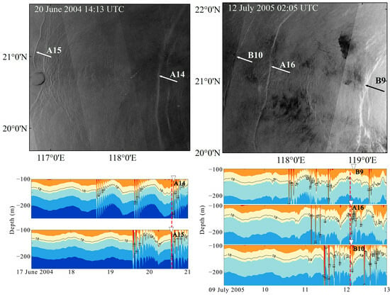
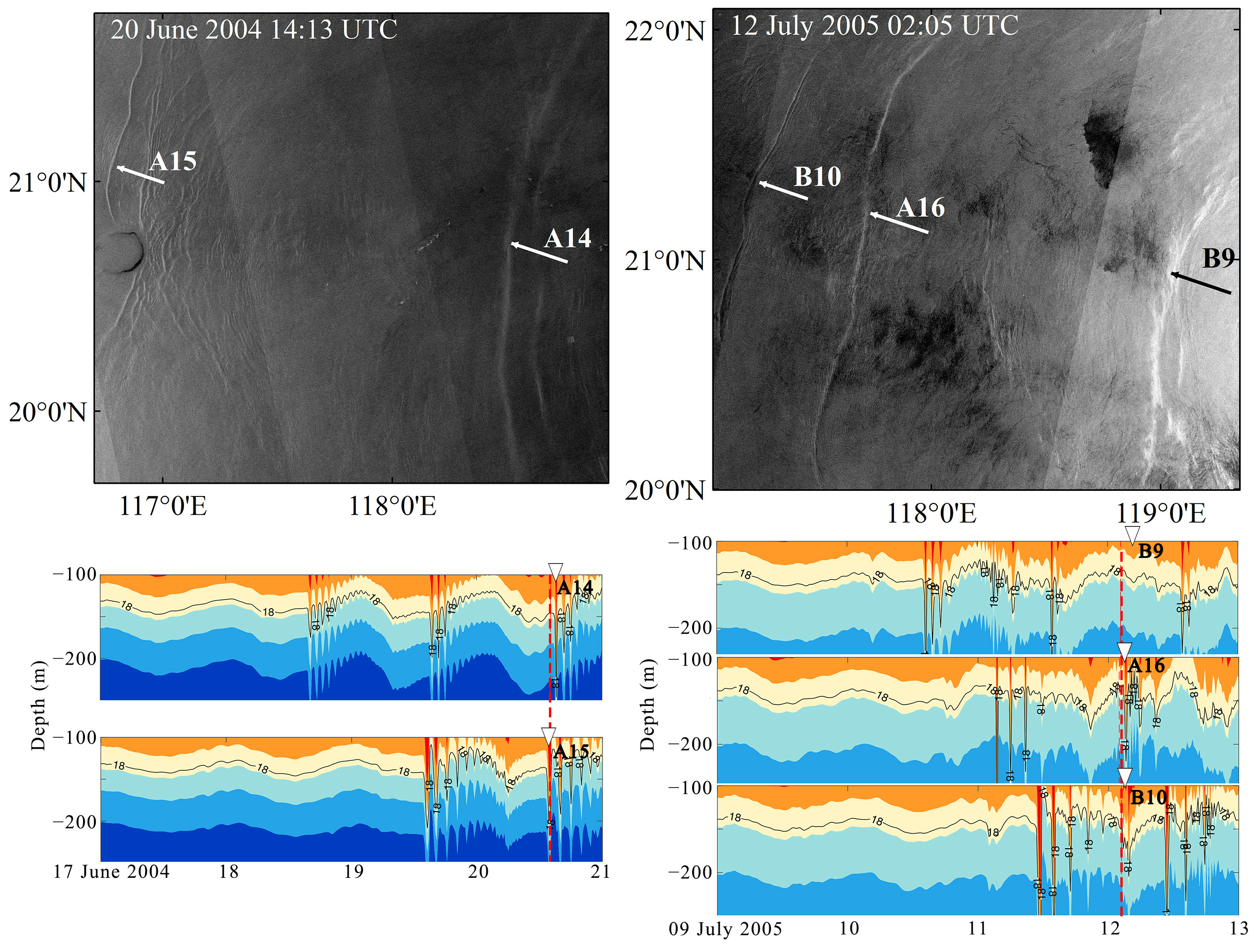
| A14 | 118.57°E | Envisat-WSS 20 June 2004 | DTP |
| A15 | 116.80°E | ||
| B9 | 119.03°E | Envisat-WSS 7 December 2005 | TTP |
| A16 | 117.70°E | ||
| B10 | 117.18°E | ||
| A17 | 118.50°E | Envisat-WSS 8 December 2006 | TTP |
| B11 | 117.63°E | ||
| A18 | 118.70°E | Envisat-WSS 9 November 2003 | TTP |
| B12 | 117.61°E | ||
| A19 | 116.87°E | ||
| A20 | 119.89°E | Envisat-WSS 22 November 2006 | DTP |
| A21 | 119.91°E | ERS-2 IMS 19 April 2007 | TTP |
| A22 | 118.82°E | ERS-2 IMS 16 February 2010 | STP |
| A23 | 118.76°E | Envisat-WSS 28 August 2006 | STP |
Disclaimer/Publisher’s Note: The statements, opinions and data contained in all publications are solely those of the individual author(s) and contributor(s) and not of MDPI and/or the editor(s). MDPI and/or the editor(s) disclaim responsibility for any injury to people or property resulting from any ideas, methods, instructions or products referred to in the content. |
© 2024 by the authors. Licensee MDPI, Basel, Switzerland. This article is an open access article distributed under the terms and conditions of the Creative Commons Attribution (CC BY) license (https://creativecommons.org/licenses/by/4.0/).
Share and Cite
Zeng, K.; Lyu, R.; Li, H.; Suo, R.; Du, T.; He, M. Studying the Internal Wave Generation Mechanism in the Northern South China Sea Using Numerical Simulation, Synthetic Aperture Radar, and In Situ Measurements. Remote Sens. 2024, 16, 1440. https://doi.org/10.3390/rs16081440
Zeng K, Lyu R, Li H, Suo R, Du T, He M. Studying the Internal Wave Generation Mechanism in the Northern South China Sea Using Numerical Simulation, Synthetic Aperture Radar, and In Situ Measurements. Remote Sensing. 2024; 16(8):1440. https://doi.org/10.3390/rs16081440
Chicago/Turabian StyleZeng, Kan, Ruyin Lyu, Hengyu Li, Rongqing Suo, Tao Du, and Mingxia He. 2024. "Studying the Internal Wave Generation Mechanism in the Northern South China Sea Using Numerical Simulation, Synthetic Aperture Radar, and In Situ Measurements" Remote Sensing 16, no. 8: 1440. https://doi.org/10.3390/rs16081440