

MRFA-Net: Multi-Scale Receptive Feature Aggregation Network for Cloud and Shadow Detection
1
Collaborative Innovation Center on Atmospheric Environment and Equipment Technology, Nanjing University of Information Science and Technology, Nanjing 210044, China
2
College of Automation, Nanjing University of Information Science and Technology, Nanjing 211004, China
*
Author to whom correspondence should be addressed.
Remote Sens. 2024, 16(8), 1456; https://doi.org/10.3390/rs16081456
Submission received: 13 March 2024
/
Revised: 8 April 2024
/
Accepted: 17 April 2024
/
Published: 20 April 2024
(This article belongs to the Special Issue Advanced Artificial Intelligence for Remote Sensing: Methodology and Applications)
Abstract
:The effective segmentation of clouds and cloud shadows is crucial for surface feature extraction, climate monitoring, and atmospheric correction, but it remains a critical challenge in remote sensing image processing. Cloud features are intricate, with varied distributions and unclear boundaries, making accurate extraction difficult, with only a few networks addressing this challenge. To tackle these issues, we introduce a multi-scale receptive field aggregation network (MRFA-Net). The MRFA-Net comprises an MRFA-Encoder and MRFA-Decoder. Within the encoder, the net includes the asymmetric feature extractor module (AFEM) and multi-scale attention, which capture diverse local features and enhance contextual semantic understanding, respectively. The MRFA-Decoder includes the multi-path decoder module (MDM) for blending features and the global feature refinement module (GFRM) for optimizing information via learnable matrix decomposition. Experimental results demonstrate that our model excelled in generalization and segmentation performance when addressing various complex backgrounds and different category detections, exhibiting advantages in terms of parameter efficiency and computational complexity, with the MRFA-Net achieving a mean intersection over union (MIoU) of 94.12% on our custom Cloud and Shadow dataset, and 87.54% on the open-source HRC_WHU dataset, outperforming other models by at least 0.53% and 0.62%. The proposed model demonstrates applicability in practical scenarios where features are difficult to distinguish.
1. Introduction
In the 1960s, the first meteorological remote sensing satellite, “TIROS”, was launched in the United States, marking a significant milestone in human history. Since then, humanity has been able to conduct the comprehensive, all-weather monitoring of Earth from space, propelling satellite remote sensing into an era of rapid development. Remote sensing technology has improved our grasp of surface data. Cloud and shadow detection is crucial in this field, helping to assess land cover and to understand solar energy distribution, thus benefiting industries like agriculture and renewable energy. Observing cloud shadow patterns also aids in climate analysis, weather forecasting, and disaster prevention. Based on statistics from the International Satellite Cloud Climatology Project (ISCCP) [1], the current cloud cover rate on Earth’s surface is maintained at about 60% to 70%. Therefore, detecting clouds and cloud shadows in remote sensing imagery is a key and fundamental step in analyzing and utilizing remote sensing data.
Historically, conventional detection methods have primarily consisted of thresholding techniques [2,3] and manual feature extraction approaches [4]. These methods analyze the spectral features of various bands of remote sensing images and set thresholds in order to segregate clouds and cloud shadows from other terrains. The features are typically obtained through extensive manual sample analyses. A representative method is the Fmask algorithm, proposed by Zhu et al. [5], which calculates terrain and cloud features using satellite image data from the top of atmosphere (TOA) reflectance and brightness temperatures. These features are then used to segment remote sensing images by establishing specific thresholds. Subsequently, with this enhancement in remote sensing resolution, some improved methods targeting more diverse features were introduced, including MFmask (mountains Fmask) [6] and Tmask (multitemporal mask) [7]. However, many of these features are limited to the red, green, blue, and near-infrared bands, rendering many detection methods based on multiple infrared bands unusable. Furthermore, these approaches often heavily rely on prior knowledge, are intricate in practical application, and have suboptimal detection accuracy.
In recent years, deep learning has undergone explosive development, garnering attention for its impressive performance across various domains, including the field of remote sensing imagery. Deep learning techniques have the ability to automatically capture subtle feature information that is often challenging for manual methods [8], resulting in high accuracy rates. Models based on convolutional neural networks (CNNs) [9,10,11] have demonstrated exceptional prowess in image classification tasks, setting the stage for the development of pixel-level classification tasks, commonly referred to as semantic segmentation. Marc et al. [12] implemented the detection and classification of five types of targets, including clouds and cloud shadows, based on the U-Net [13] framework. Furthermore, they validated the method’s generalization capability across different satellite sensors. Wu et al. [14] built upon the FCN [15] framework for GF-1 WFV (Gaofen-1 Wide Field View) remote sensing images, employing a fusion of CNN-extracted low-level and high-level features in order to generate cloud probability maps. However, traditional models based on encoder and decoder stages significantly lose image information during down-sampling and struggle to effectively recover image details during up-sampling [16]. Additionally, most of the aforementioned works directly train semantic segmentation models designed for natural images on remote sensing detection datasets without specifically optimizing and designing the model structure for cloud detection tasks, thus leading to poor performance for challenging samples [17]. With ongoing research in cloud detection tasks, researchers have identified that designing more effective methods for multi-scale feature extraction and fusion, tailored to the characteristics and challenges of cloud detection tasks, is one of the key technologies to improve the accuracy of cloud detection algorithms. Yang et al. [18] proposed CDnet for low-resolution remote sensing thumbnail images, enhancing cloud detection accuracy in low-resolution images through feature pyramids and edge refinement modules. Li et al. [19] specifically targeted medium- to high-resolution remote sensing images, designing a multi-scale convolutional feature fusion (MSCFF) method to improve cloud detection accuracy, and validating the effectiveness of the method across remote sensing images from different sensors. However, the computational complexity of these models significantly increases. When dealing with complex remote sensing images, researchers may find that performance is still constrained due to the number of paths and pyramid layers.
Attention mechanisms [20,21,22] are currently a pivotal research topic in deep learning. An effective attention mechanism module can further elevate the performance ceiling of a model by enhancing the capturing of pertinent feature information from channels or spaces. In 2018, the convolutional block attention module (CBAM) [23], a convolution-implemented hybrid attention mechanism, featuring adaptively refined features from both channel and spatial perspectives, led to a significant boost in model performance. In 2021, the vision transformer (ViT) [24] bridged the divide between computer vision (CV) and natural language processing (NLP), feeding images into multi-head attention structures in an encoded form, and greatly enhancing global information capture. Chen et al. [25] introduced ViT into CNN networks, proposing a dual-branch network for cloud and cloud shadow detection that achieves high accuracy, while also demonstrating good robustness and generalization capabilities. However, this approach led to parameter inflation. In response to this issue, Hu et al. [26] replaced the dual-branch network’s ViT with the less parameter-intensive EdgeViT, resulting in faster inference speeds for the network. Despite this improvement, the parameter count remains substantial, and these networks require large datasets for fitting. Underfitting may occur when the sample size is small.
Few models specifically address cloud and cloud shadow segmentation, owing to the unique distribution and complexity. Clouds and shadows in remote sensing images exhibit significant variations in size, shape, and structure, with inconsistent brightness and intricate boundaries. Current semantic models often miss these details, resulting in blurred boundaries. However, multi-scale feature fusion enhances detail and edge clarity. Considering the diverse terrain features and cloud shadow variations across seasons and regions, models require strong global understanding. Challenges such as noise, pseudo shadows, and terrains mimicking cloud characteristics further complicate the segmentation, leading to frequent misidentifications. In response to the aforementioned challenges, this paper introduces a multi-scale encoder and decoder, which can capture intricate details and enhance global information understanding, precisely capturing features and restoring spatial resolution. Additionally, it can fill in detailed information gaps by merging information from both deeper and shallower layers. The primary contributions of this paper and innovations of our model are as follows:
- (1)
- For cloud and cloud shadow detection in remote sensing images, a novel framework called the MRFA-Net is proposed. This model fully utilizes rich features to address the misidentification of blurry features, small objects, and abstract characteristics in detection. The network is end-to-end trainable, significantly simplifying the process of cloud and cloud shadow detection.
- (2)
- Previous methods have overlooked the feature information across different scales. We propose the asymmetric feature extractor module (AFEM) and the multi-scale attention to capture irregular information across multiple scales and to enhance both local and global semantic information. To address the issue of information loss due to direct continuous up-sampling in previous networks, the multi-path decoder module (MDM) and the global feature refinement module (GFRM) are introduced. These modules combine feature information from different receptive fields with the feature fusion module (FFM) and optimize the information before decoding.
- (3)
- We evaluated the model on two remote sensing datasets with diverse environmental scenarios, including tests in challenging conditions. The outcomes demonstrate that the MRFA-Net is quite accurate and reliable when compared to previous deep learning based algorithms.
2. Methods
2.1. Overview
The multi-scale model architecture proposed in this paper effectively identifies clouds and cloud shadows, accurately generating clear segmentation masks. The overall structure of the model is illustrated in Figure 1, and is primarily composed of an encoder stage and a decoder stage. Specifically these phases are conducted as follows: (1) In the encoding phase, each encoder encompasses the AFEM and multi-scale attention. To address the irregular and blurry features in remote sensing images, the AFEM is tasked with capturing local information across various scales while reducing the resolution. The multi-scale attention is tailored to the features of different phases, and employs corresponding attention strategies, utilizing MSA and MCA. (2) In the decoding phase, the features are refined and decoded by the MDM and GFRM. Through the FFM, features from both deep and shallow layers, as well as from different branches, are integrated. For features with lower resolutions but a higher number of channels, decoding is carried out using the MDM. Conversely, for features with a larger resolution, the designed GFRM further refines these features before decoding.
2.2. Asymmertric Feature Extractor Module
The asymmetric feature extractor module (AFEM) is crucial for accurately segmenting cloud shadow remote sensing images, with its core task being the identification and capture of the diverse features of cloud shadows. In recent years, several segmentation models have employed multi-scale feature extraction modules, such as Dual-Branch Net and MCANet, achieving certain results. However, these models often tend to focus on refining information or utilize large-scale convolutions in breadth, attempting to capture as much comprehensive feature information as possible in a single process, without considering deeper features. This leads to an explosion in the number of model parameters, and the redundancy of information can result in model performance instability. Therefore, a balanced multi-scale feature extraction module should not only prioritize performance, but also accurately capture pertinent feature information.
To address the aforementioned issues, we introduce the AFEM. Its structure is illustrated in Figure 2. Input features first pass through a point-wise convolution layer and a 3 × 3 convolution layer, thus adjusting the channel number to the desired output channels. Concurrently, a residual mechanism is introduced. Subsequently, the features are split into four subsets (where ) along the channel dimension. Each of these subsets is processed through a 1 × 1 convolution layer and asymmetric multi-scale convolution layers with varying kernel sizes, thus yielding multi-scale feature outputs. The formula is as follows:
where MFO denotes a multi-scale feature output, Conv( ) refers to point-wise convolution, and SConv( ) corresponds to the combination of strip convolutions.
Given that the features from different levels retain the spatial information of varying dimensions, it is essential to account for the discrepancies among features of different depths. In response to this, the asymmetric convolution layer scales in the AFEM can be adjusted. The lengths of stripe convolutions k1, k2, and k3 are tunable parameters. For shallower features with a larger resolution, using a more extensive convolution kernel captures a broader scope of spatial information. Conversely, for deeper features with a smaller resolution, employing a smaller kernel refines the capability to capture details. Therefore, when the feature resolution exceeds 64 × 64, the lengths of the stripe convolutions are set to 3, 7, and 11. For resolutions below 64 × 64, these lengths are adjusted to 3, 5, and 7. Consequently, the entire AFEM can capture feature information of various sizes in a multi-scale manner during the down-sampling process.
2.3. Multi-Scale Attention
Grasping the context of spatial information plays a pivotal role in remote sensing image segmentation. Even minor positional changes in the image can significantly influence the model’s final output. Hence, the integration of spatial attention mechanisms is crucial. Most spatial attentions operate on a linear structure, only accepting feature information from a fixed receptive field. This approach limits the model’s ability to process multi-scale spatial information. To address this, we integrate multi-scale spatial attention (MSA) and multi-scale channel attention (MCA) into our model. These two modules operate in the first half and the second half of the encoding phase, respectively. MSA serves as the feature enhancement mechanism in the spatial dimension, bolstering the understanding of cloud and cloud shadow positional information. It divides the features into four branches, feeds them into the spatial attention mechanism after different convolutions, stacks them, and finally modifies the number of channels through point-wise convolution. In contrast, MCA augments features in the channel dimension, enhancing the control over the weights between different channels and amplifying the model’s generalization capabilities. It splits the features into four branches, stacks them after different convolutions, feeds them into the channel attention mechanism, and finally modifies the number of channels through point-wise convolution.
The structure of the MSA is illustrated in Figure 3. It comprises four parallel spatial attention modules (SAMs), three passing through a 3 × 3 dilation convolution layer and one passing through a 3 × 3 convolution. These convolution layers utilize different dilation rates of 3, 5, and 7, respectively. This not only expands the receptive field, but also facilitates the assimilation of multi-scale features, thus amplifying the model’s spatial understanding. SAMs operate adaptively, focusing on the intricate spatial details within the locality. The pixel values across all channels in the image sequentially undergo both maxpool and avgpool layers, allowing for the reallocation of the appropriate weights. This approach enables the model to selectively concentrate on salient features. Finally, the processed features are stacked and sent through a point-wise convolution layer to be input into the subsequent module.
The procedure of the MSA can be delineated by the subsequent equation:
where MSAO represents the multi-scale spatial attention output, Xi denotes the parallel inputs convolved with different convolutional kernels, and SA( ) signifies the spatial attention operation.
The structure of the MCA module is depicted in Figure 4. Similarly to the MSA, it also encompasses four parallel processes, but it employs the channel attention mechanism (CAM). The CAM measures based on the average and maximum value of information within a channel. This approach enables the CAM to automatically adjust the weights among different channels, capturing channel-specific information and thereby enhancing the comprehension of global data. After convolution, the stacked multi-scale features are combined in the channel dimension through channel attention. The procedure of the MCA can be articulated as follows:
where MCAO denotes the multi-scale channel attention output, Yi represents the parallel input of the network following operations with diverse convolution kernels, and CA( ) signifies the channel attention operation.
Considering the variance in the feature scale sizes contained within the different depths of features, we utilize distinct attention mechanisms in the encoding phase to optimize information. Since shallower features have a larger resolution and fewer channels, they are more sensitive to spatial attention mechanisms. In contrast, deeper features, with a smaller resolution and a higher number of channels, are better optimized with channel attention. Thus, when the feature resolution exceeds 64 × 64, MSA is used to further refine features, reducing noise and amplifying valuable information. Conversely, when the feature resolution is below 64 × 64, MCA is employed to optimize multi-scale global information. Typically, both MSA and MCA not only enhance the receptive field, but also capture effective spatial data and multi-scale channel information through their designed combination.
2.4. Multi-Path Decoder Module
The decoder is a crucial component in semantic segmentation models, responsible for restoring spatial resolution. Traditional models typically have a simplistic decoding section. While these models may be somewhat reliable, they are constrained by receptive field limitations, making it challenging to recover multi-scale information. Additionally, the simple up-sampling of features often results in significant detail losses. To address these challenges, we introduce a multi-path decoder module (MDM) that fuses information across different depths and restores images at multiple scales. Furthermore, our designed global feature refinement module refines the information during up-sampling.
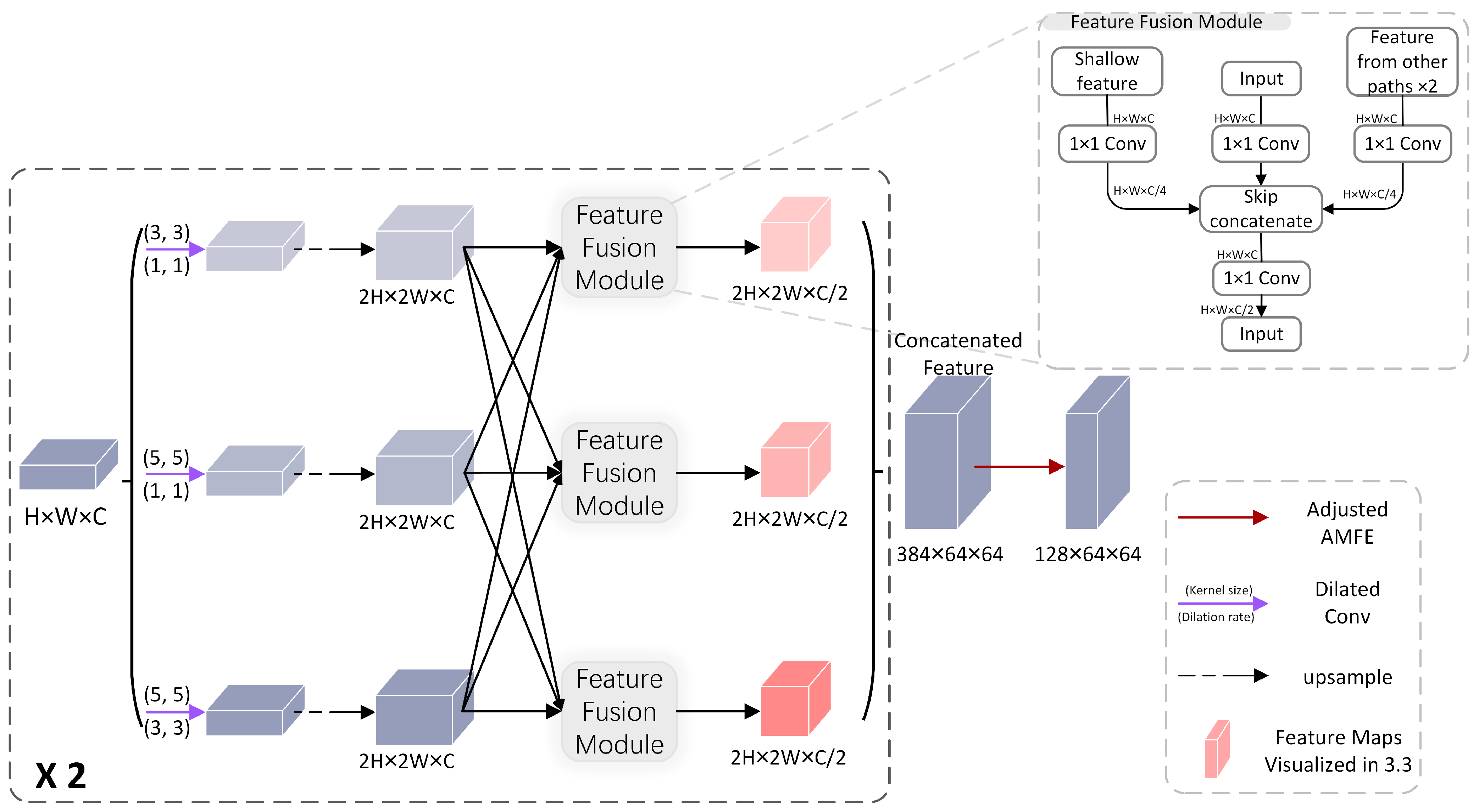
The specific structure of the MDM is depicted in Figure 5, targeting the deeper features with a larger number of channels. The gray section in the figure represents the feature fusion module, which is used to integrate features from different receptive fields, thus reducing information loss. The multi-path decoder consists of three parallel branches, with each branch receiving features from dilated convolutions with varying receptive fields. Each path also contains two up-sampling modules, employing bilinear interpolation. Starting with an input feature size of 16 × 16, the sizes transition to 16 × 16 and 32 × 32 post-up-sampling. Solely relying on a single channel and deep features can sacrifice much of the finer details. Consequently, we introduce a feature fusion module (FFM), as shown in the top right gray dashed rectangle of Figure 5. Utilizing a 1 × 1 convolution layer, we can halve the channel count of the shallower features and other branches. The multi-scale features are then fused using the concatenate operation. This approach ensures the preservation of semantic information across different scales within the channel dimension. Moreover, the FFM is also integrated into subsequent decoding processes.
2.5. Global Feature Refinement Module
To refine detailed information and expand the receptive field, specifically for features at the tail end of the model decoding with higher resolutions, we propose a global feature refinement module (GFRM). This is a lightweight module aimed at refining global context information. The architecture is depicted in Figure 6. The GFRM primarily employs NMF matrix factorization [27] to denoise and enhance the information [28,29,30], and also uses the backpropagation through time [31] algorithm for backpropagating gradients [32,33]. The information from one channel of an image can be viewed as a matrix , where its pertinent information is embedded in one or more low-rank subspaces. It can then be conceived that the decomposition of can be represented by a dictionary matrix and the corresponding encoding , for which the formula is as follows:
For common networks, the feature tensor output by the network is . If the tensor is unfolded into matrices, those can be represented as a matrix . When the module relies on context information, the hidden assumption is that the superpixels represented by the “global information” are intrinsically related. These superpixels can actually be represented as linear combinations of a set of bases. Typically, is of a low rank. can be decomposed into two parts: the low-rank “global information” and the residual .
This process can be viewed as an optimization process where the clean information subspace is determined through algorithmic optimization, discarding the residual. We model the global information description using the following function:
where represents the reconstruction error, derived from the distribution of the residual term ; and denote regularization for the dictionary matrix and the coefficient matrix , respectively; and is the optimization algorithm for the objective function, and is the key to this module.
In this paper, non-negative matrix factorization is adopted. The module includes a matrix decomposition model within two linear transformations:
wherein is the lower linear transformation, mapping the input to the feature space, and is the low-rank feature subspace derived from the corresponding non-negative matrix factorization decomposition. The output is then transformed using the upper linear transformation .
Furthermore, it is necessary to compute the gradient of the feature decomposition for backpropagation, ensuring its differentiability. In this paper, we adopt the backpropagation through the time algorithm. Matrix decomposition is abstracted to apply implicit differentiation. The GFRM reduces computational complexity while discarding global redundant information, thus enhancing the understanding of hierarchical information and further refining detail information.
3. Experimental Analysis
3.1. Datasets
3.1.1. Cloud and Cloud Shadow Dataset
The dataset’s remote sensing images were primarily obtained from the U.S. Landsat 8 satellite, and supplemented by high-resolution remote sensing images selected from Google Earth (GE). The Landsat 8 satellite is equipped with a land imager with nine bands and a thermal infrared sensor with two bands. The high-definition satellite images from Google Earth are mainly captured with the QuickBird satellite and the WorldView-4 satellite. The QuickBird satellite is capable of acquiring high-quality remote sensing images, boasting a satellite imagery resolution of up to 0.61 m. Additionally, it possesses the capability to collect four-band spectral resolution images with resolutions ranging from 2.44 to 2.88 m. The WorldView-4 satellite is equipped to capture high definition remote sensing images at a resolution of 0.3 m, while also being able to acquire multispectral images at a resolution of 1.24 m. This dataset primarily utilizes the second blue band (0.450–0.515 μm), the third green band (0.525–0.600 μm), and the fourth red band (0.630–0.680 μm). Owing to the large original image sizes and GPU memory constraints, the original images were uniformly cropped to a resolution of 224 × 224, ensuring easy training. In total, 10,843 images were obtained, and they were grouped in an 8:2 ratio to serve as the training and validation sets, respectively.
To ensure that the dataset was representative and reflected real world scenarios, we utilized images from various angles, altitudes, and backgrounds at specific ratios. Image backgrounds encompass various terrains, including cities, sandy areas, farmlands, seas, etc. Moreover, since this study focused on clouds and cloud shadows, some filtering was performed on the labels, removing other terrain labels and retaining only cloud and cloud shadow labels, as well as some terrain labels that were similar to cloud features for training.
3.1.2. HRC_WHU Dataset
To further test the model’s generalization capability, we also utilized the HRC_WHU high-resolution cloud dataset. The data, sourced from [34] the Wuhan University laboratory, consist of 150 high-resolution remote sensing images, with resolutions primarily ranging from 0.5 m to 15 m and an original size of 1280 × 720. The terrain types include vegetation, snow, desert, cities, and water surfaces. Similarly, owing to GPU memory constraints, the images were cropped into 224 × 224 sub-images for training, as shown in Figure 7. This resulted in a total of 3600 images, which were grouped in an 8:2 ratio to serve as the training and validation sets, respectively. Finally, manually annotated cloud shadow were added to the labels. Black, white, and gray represent categories, corresponding to the background, clouds, and cloud shadows, respectively.
In both datasets, the label data were initially in the form of images, with different colors representing different categories. During training, we mapped the colors representing categories onto different channels for training purposes. Finally, for visualization, we converted the categories on the channels back to RGB colors for visualization.
3.2. Experiment Details
All experiments were implemented using the PyTorch framework, version 1.10.1. The utilized GPU was NVIDIA’s RTX2080Ti, with a memory of 11GB. The batch sizes for training on both datasets were set to 16, with training epochs totaling 300. The optimizer used was Adam. The learning rate was managed using a step-wise learning rate (StepLR), starting at 0.001, with a decay factor of 0.9. The learning rate was updated every three epochs. The formula for calculating the learning rate was as follows:
In this study, represents the learning rate at the nth training iteration, is the initial learning rate, β is the decay coefficient, and s is the update interval. The loss function used in training is the cross-entropy loss, and its formula is as follows:
When evaluating the performance of the model, we used metrics such as pixel accuracy (PA), mean pixel accuracy (MPA), and mean intersection over union (MIoU) to assess the model’s performance. Their calculation formulas are as follows:
where represents precision, which is the proportion of pixels in the prediction that are correctly identified; stands for recall, denoting the proportion of pixels in the ground truth that are correctly predicted; is the number of classes; is the count of pixels of class i predicted as class j; is the number of pixels of class j predicted as class i; and is the count of pixels that belong to class i and are predicted as class i.
3.3. Parameter Analysis
3.3.1. Ablation Experiments
To evaluate the contribution of the modules to the overall network, we conducted ablation experiments on the key components of the model separately on the HRC_WHU dataset and the Cloud and Cloud Shadow Dataset (CCSD), using PA and MIoU metrics for the evaluation.
To assess the impact of the AFEM, we replaced the AFEM with a max pooling layer of stride 2, denoted as the MFRA-Net/AFEM−. For multi-scale attention, we substituted the module with two 3 × 3 convolution layers with a residual mechanism, denoted as the MFRA-Net/MA−. For the multi-path decoder, we directly replaced the entire module with linear bilinear interpolation up-sampling, denoted as the MFRA-Net/Decoder−. To investigate the role of the GFRM, we simply removed it, denoted as the MFRA-Net/GFRM−.
The ablation experiments for each module are shown in Table 1. The improvements on the HRC_WHU Dataset were noticeable, whereas further optimization effects were observed for the CCSD Dataset. With the introduction of the AFEM, the MIoU metric on the two datasets increased by 0.37% and 0.16%, respectively. With the introduction of the multi-scale attention, the MIoU metric on the two datasets increased by 1.35% and 0.39%, respectively. With the introduction of the multi-path decoder, the MIoU metric increased by 0.54% and 0.33%, respectively. After the introduction of the GFRM, the increase in the MIoU metric was 1.51% and 0.51%, respectively. Additionally, the AFEM and MDM can, to a certain degree, reduce the model parameters and accelerate the model’s inference speed.
As shown in Figure 8, the heat map provides a clearer depiction of the feature extraction status. White boxes indicate accurately extracted features, while red boxes signify false detection. Yellow boxes indicate missed detections, and red circles denote the presence of significant noise. With the introduction of multi-scale attention, the occurrence of missed detections was substantially reduced. The network could better capture faint and minute targets, attributable to multi-scale attention’s ability to greatly amplify the ability to capture vital features and to enhance contextual understanding. Incorporating the AFEM, the asymmetrical convolution-derived multi-scale features displayed a distinct advantage, leading to a more precise and clean boundary demarcation, and reducing instances of feature conglomeration. Introducing the MDM reduced the loss of information due to the fusion of multi-scale features, and also mitigated missed detections to some extent. The impact of integrating the GFRM on the model was quite evident; noise from clouds and backgrounds in the image was markedly eliminated, and category demarcations were clearer. This is because the GFRM further refines the features extracted by the model, comprehending semantic information globally through the matrix decomposition of back-propagated gradients, eliminating redundant features while reinforcing the necessary ones.
3.3.2. Analysis of the Decoder Paths
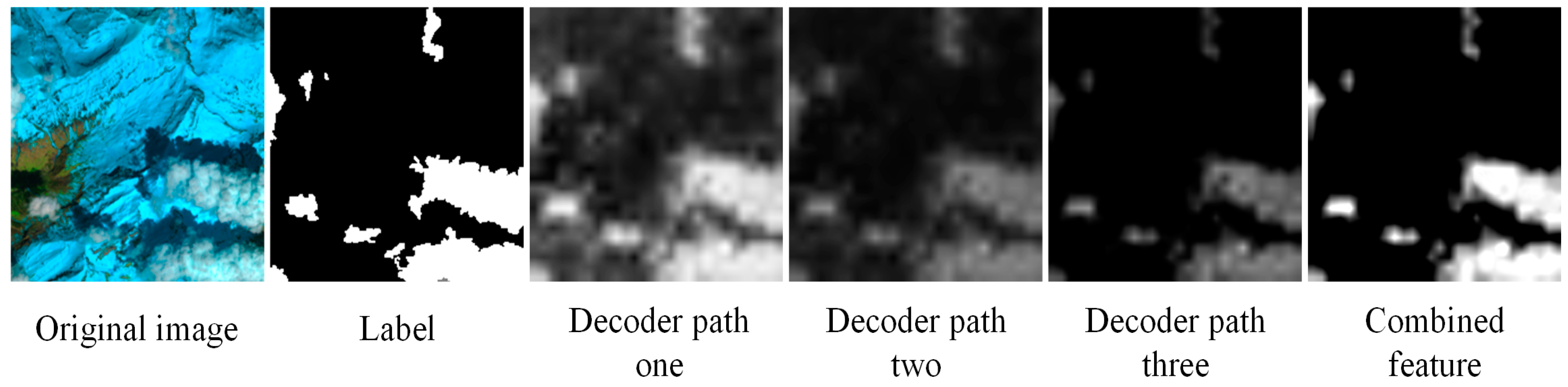
Additionally, to explore the impact of the MDM, we visualized the features from different paths. As depicted in Figure 9, in decoder path one, although feature extraction was most prominent, it encompassed considerable noise and impure extracted features, potentially giving rise to false detections. In decoder path two, we observed the presence of noise as well as certain phenomena of feature extraction omissions. In decoder path three, despite a more accurate range of feature extraction, we observed more instances of feature extractions being missed. Feature fusion can aptly resolve this issue. Each path contains rich features, and the receptive fields of different paths vary. A smaller receptive field is more sensitive to the detection of smaller targets, whereas a larger receptive field excels in detecting larger, sheet-like targets. Moreover, shallow features, even though they encompass a broader receptive field and contain more information, are often laden with noise, redundant features, and exhibit a degree of ambiguity. In contrast, deeper features, despite their high purity in extraction, tend to lose many intricate details. The fusion of features from different branches effectively addresses this issue. When combined with the subsequent GFRM, it could precisely retain multi-scale edge details and eliminate redundant features, thus resulting in accurate target detection.
3.3.3. Parameters of AFEM
The AFEM is a highly effective multi-scale module that learns local information through features with varying receptive fields. Among these, the sizes of the strip convolutions, denoted as , , and , play a crucial role in feature extraction. To select the optimal parameters, we compared five sets of different convolution kernel sizes in this experiment, as shown in Table 2. Net-S and Net-L had fixed convolution sizes at different stages, while Net-AS and Net-AL adaptively used different kernel sizes at different stages. The experiments were conducted on the Cloud and Cloud Shadow Dataset, as outlined in Table 3. It is evident that adapting the convolution kernels at different stages yielded better results when compared to a static approach. Moreover, even when dynamically adjusting the kernels at different stages, the selection of appropriate strip convolution kernel sizes remained crucial. Among the four compared categories, the MFRA-Net was shown to be more effective, owing to its well-considered parameter settings.
3.4. Comparison Test of the Cloud and Cloud Shadow Dataset
To further evaluate the performance of the proposed network, we conducted comparative experiments on a dataset, juxtaposing the MRFA-Net with the currently prevalent and outstanding semantic segmentation models, including the U-Net, FCN, SegNet [35], PSPNet [36], DeepLabv3+ [37], ShuffleNetV2 [38], DABNet [39], and CCNet [40]. Moreover, we also compared this with some of the latest networks designed for remote sensing, namely the CSAMNet and Dual-branch Network (DBNet). The MRFA-Net exhibited superior performance, outperforming the next best network by 0.53% in terms of the MioU. The results are as shown in Table 4.
Based on the results, our model still maintained optimal performance on the WHU_HRC Dataset. It outperformed the second-best model by 0.62% on the MIOU metric. Specifically for this dataset, we mainly compared the results on images with similar cloud features, as illustrated in Figure 10. In the first row, our cloud and snow features were somewhat similar, with only slight differences in their edge features. During recognition, thanks to the rich multi-scale features and modules that enhance feature comprehension, our model accurately identified the general contour. Only a small portion of scattered snow on the right side was recognized as a cloud. In contrast, other networks’ ability to demarcate similar features dropped significantly. For the second row, we chose an image where clouds and accumulated snow intertwine. The snow features appeared brighter compared with the cloud. Our network distinguished such features with relative ease. However, our network recognized the long, intermittent snow strips. Meanwhile, other networks struggled to accurately differentiate the cloud and snow features below. In the third row, we selected an image displaying a cloud adjacent to accumulated snow. The cloud features were deeper, distinctly different from the snow. All networks could identify the general contour, but when it came to the edge features where the cloud and snow overlapped, our network clearly outperformed the others. This superiority stems from our modules being designed for intricate feature refinement. Beyond capturing features of different scales, the attention mechanism employs smaller convolution kernels in the deeper layers. The global information refinement further aids the network in better understanding both local and global contexts, thereby achieving improved performance.
3.5. Comparison Test of the HRC_WHU Dataset
To further investigate the performance of the MRFA-Net and validate the generalizability of our model, we conducted comparative experiments on the HRC_WHU Dataset. The HRC_WHU Dataset possesses features that are stylistically inconsistent with the Cloud and Cloud Shadow Dataset. For example, sandy terrains under strong light share similar features with thin cloud layers, making them easily confusable. Nevertheless, the model should be able to accurately segment the edges between the background and the target, extracting detailed features. We continued to compare our results with some popular models. The experimental results are presented in Table 5.
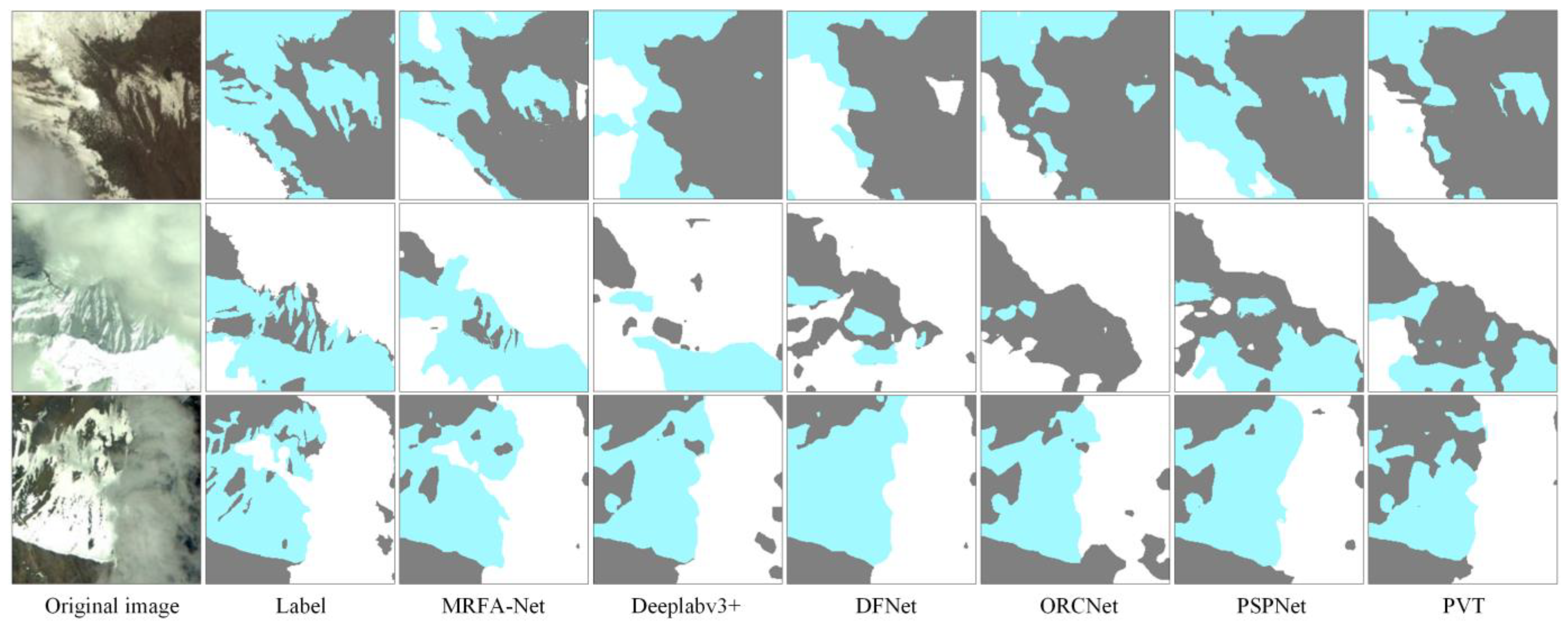
As illustrated in Figure 11, we mainly compared the results on images with similar cloud features. In the first row, our cloud and snow features were somewhat similar, with only slight differences in their edge features. During recognition, thanks to the rich multi-scale features and modules that enhance feature comprehension, our model accurately identified the general contour. Only a small portion of scattered snow on the right side was recognized as a cloud. In contrast, other networks’ ability to demarcate similar features dropped significantly. For the second row, we chose an image where the cloud and accumulated snow intertwined. The snow features appeared brighter when compared with the cloud. Our network distinguished such features with relative ease. It achieved the recognition of the long, intermittent snow strips. Conversely, other networks struggled to accurately differentiate the cloud and snow features below. In the third row, we selected an image displaying a cloud adjacent to accumulated snow. The cloud features were deeper, distinctly different from the snow.
4. Discussion
4.1. Advantages of the Method
This paper introduces an efficient, multi-scale cloud and cloud shadow detection method with low computational complexity. When compared to traditional approaches, our method significantly reduces the manual labor in data labeling, handcrafted feature extraction, and setting feature thresholds. It does not rely on prior knowledge and addresses the inherent challenge of noise resilience in traditional thresholding techniques. As a result, it achieves substantially higher accuracy and possesses greater versatility when compared to previous methods. Furthermore, when compared to existing semantic segmentation techniques, our network emphasizes multi-scale and multidimensionality, employing different strategies at various levels. This approach effectively captures some overlooked details and emphasizes critical features. For instance, it can distinctly identify and differentiate smaller targets and features that resemble both the background and the target. As a result, it exhibits superior performances, even on complex remote sensing image sets. It boasts strong generalization across various terrains, outstanding performance, and low computational complexity. It performs exceptionally well on both the Cloud and Cloud Shadow Dataset we collected, and the publicly available HRC_WHU Dataset.
4.2. Limitation of the Method
Although the MFRA-Net has achieved commendable results in cloud and cloud shadow detection and the network has a certain advantage in terms of parameter optimization, there is still room for improvement. Detection is the first step. In the future, we plan to incorporate temporal remote sensing data to remove and denoise images obscured by clouds and cloud shadows, thereby recovering image information. Moreover, we aim to extend this method to other types of remote sensing data, such as synthetic aperture radar (SAR) remote sensing, in order to enhance the model’s versatility across different data types.
5. Conclusions
This paper introduces the MRFA-Net for cloud and shadow detection. Its distinctive feature is the use of different strategies at various network levels based on feature characteristics, and the integration of multi-scale features, thus resulting in superior performance. This network is based on an encoder–decoder structure. During the encoding phase, multidimensional features are mainly extracted via the AFEM. The sizes of convolutional kernels vary according to feature tensor changes. Subsequently, the multi-scale attention module refines feature information. Different hierarchical features also separately adopt multi-scale spatial and channel attentions, adaptively understanding and enhancing the contextual semantic information of images. Additionally, these designs, to some extent, reduce the number of parameters, thus speeding up the model’s inference time. During the decoding phase, different approaches are adopted for features of varying sizes and characteristics. For channel-wise and smaller feature tensors, the MDM is employed for feature fusion and up-sampling. By merging features from different branches and levels, the potential for information loss is significantly reduced, making the decoding process more reliable than previous methods. For larger feature tensors, an innovative matrix decomposition GFRM, capable of backward gradient propagation, is utilized to further refine global information, eliminate redundant features, and enhance valuable information. On the Cloud and Cloud Shadow Dataset, as well as the HRC_WHU dataset, it achieved MioU scores of 94.12% and 87.54%, respectively, thus exceeding other models.
Author Contributions
Conceptualization, J.W. and Y.L.; methodology, J.W. and X.Z.; software, J.W.; validation, X.Z., X.F. and M.W.; investigation, M.W.; resources, X.F. and X.Z.; data curation, J.W.; writing—original draft preparation, J.W.; writing—review and editing, Y.L.; visualization, J.W. and X.F.; supervision, Y.L.; project administration, Y.L.; funding acquisition, Y.L. All authors have read and agreed to the published version of the manuscript.
Funding
This work was supported in part by the National Natural Science Foundation of China (61671010) and the Qing Lan Project of Jiangsu Province (B2018Q03).
Data Availability Statement
The data and the code of this study are available from the corresponding author upon request.
Conflicts of Interest
The authors declare no conflicts of interest.
References
- Rossow, W.B.; Schiffer, R.A. Advances in Understanding Clouds from ISCCP. J. Bull. Am. Meteorol. Soc. 1999, 80, 2261–2288. [Google Scholar] [CrossRef]
- Moses, W.J.; Philpot, W.D. Evaluation of atmospheric correction using bi-temporal hyperspectral images. Isr. J. Plant Sci. 2012, 60, 253–263. [Google Scholar] [CrossRef]
- Liu, X.; Xu, J.-M.; Du, B. A bi-channel dynamic thershold algorithm used in automatically identifying clouds on gms-5 imagery. J. Appl. Meteorlog. Sci. 2005, 16, 134–444. [Google Scholar]
- Tapakis, R.; Charalambides, A.G. Equipment and methodologies for cloud detection and classification: A review. Sol. Energy 2013, 95, 392–430. [Google Scholar] [CrossRef]
- Zhu, Z.; Woodcock, C.E. Object-based cloud and cloud shadow detection in landsat imagery. Remote Sens. Environ. 2012, 118, 83–94. [Google Scholar] [CrossRef]
- Qiu, S.; He, B.; Zhu, Z.; Liao, Z.; Quan, X. Improving fmask cloud and cloud shadow detection in mountainous area for landsats 4–8 images. Remote Sens. Environ. 2017, 199, 107–119. [Google Scholar] [CrossRef]
- Zhu, Z.; Woodcock, C.E. Automated cloud, cloud shadow, and snow detection in multitemporal landsat data: An algorithm designed specifically for monitoring land cover change. Remote Sens. Environ. 2014, 152, 217–234. [Google Scholar] [CrossRef]
- Wang, Z.; Xia, M.; Lu, M.; Pan, L.; Liu, J. Parameter identification in power transmission systems based on graph convolution network. IEEE Trans. Power Deliv. 2022, 37, 3155–3163. [Google Scholar] [CrossRef]
- Ayala, C.; Sesma, R.; Aranda, C.; Galar, M. A deep learning approach to an enhanced building footprint and road detection in high-resolution satellite imagery. Remote Sens. 2021, 13, 3135. [Google Scholar] [CrossRef]
- Prathap, G.; Afanasyev, I. Deep learning approach for building detection in satellite multispectral imagery. In Proceedings of the 2018 International Conference on Intelligent Systems (IS), Funchal, Portugal, 25–27 September 2018. [Google Scholar]
- Xie, W.; Fan, X.; Zhang, X.; Li, Y.; Sheng, M.; Fang, L. Co-compression via superior gene for remote sensing scene classification. IEEE Trans. Geosci. Remote Sens. 2023, 61, 5604112. [Google Scholar] [CrossRef]
- Wieland, M.; Li, Y.; Martinis, S. Multi-sensor cloud and cloud shadow segmentation with a convolutional neural network. Remote Sens. Environ. 2019, 230, 111203. [Google Scholar] [CrossRef]
- Ronneberger, O.; Fischer, P.; Brox, T. U-Net: Convolutional networks for biomedical image segmentation. In Proceedings of the Medical Image Computing and Computer-Assisted Intervention—MICCAI 2015, Munich, Germany, 5–9 October 2015. [Google Scholar]
- Wu, X.; Shi, Z. Utilizing multilevel features for cloud detection on satellite imagery. Remote Sens. 2018, 10, 1853. [Google Scholar] [CrossRef]
- Long, J.; Shelhamer, E.; Darrell, T. Fully convolutional networks for semantic segmentation. In Proceedings of the IEEE Conference on Computer Vision and Pattern Recognition, Boston, MA, USA, 7–12 June 2015. [Google Scholar]
- Jeppesen, J.H.; Jacobsen, R.H.; Inceoglu, F.; Toftegaard, T.S. A cloud detection algorithm for satellite imagery based on deep learning. Remote Sens. Environ. 2019, 229, 247–259. [Google Scholar] [CrossRef]
- Yan, Z.; Yan, M.; Sun, H.; Fu, K.; Hong, J.; Sun, J.; Zhang, Y.; Sun, X. Cloud and cloud shadow detection using multilevel feature fused segmentation network. IEEE Geosci. Remote Sens. Lett. 2018, 15, 1600–1604. [Google Scholar] [CrossRef]
- Yang, J.; Guo, J.; Yue, H.; Liu, Z.; Hu, H.; Li, K. CDnet: CNN-based cloud detection for remote sensing imagery. IEEE Trans. Geosci. Remote Sens. 2019, 57, 6195–6211. [Google Scholar] [CrossRef]
- Li, Z.; Shen, H.; Cheng, Q.; Liu, Y.; You, S.; He, Z. Deep learning based cloud detection for medium and high resolution remote sensing images of different sensors. ISPRS J. Photogramm. Remote Sens. 2019, 150, 197–212. [Google Scholar] [CrossRef]
- Qu, Y.; Xia, M.; Zhang, Y. Strip pooling channel spatial attention network for the segmentation of cloud and cloud shadow. Comput. Geosci. 2021, 157, 104940. [Google Scholar] [CrossRef]
- Zhang, C.; Weng, L.; Ding, L.; Xia, M.; Lin, H. CRSNet: Cloud and cloud shadow refinement segmentation networks for remote sensing imagery. Remote Sens. 2023, 15, 1664. [Google Scholar] [CrossRef]
- Chen, Y.; Tang, L.; Huang, W.; Guo, J.; Yang, G. A novel spectral indices-driven spectral-spatial-context attention network for automatic cloud detection. IEEE J. Sel. Top. Appl. Earth Obs. Remote Sens. 2023, 16, 3092–3103. [Google Scholar] [CrossRef]
- Woo, S.; Park, J.; Lee, J.-Y.; Kweon, I.S. CBAM: Convolutional block attention module. In Proceedings of the European Conference on Computer Vision (ECCV) 2018, Munich, Germany, 8–14 September 2018. [Google Scholar]
- Dosovitskiy, A.; Beyer, L.; Kolesnikov, A.; Weissenborn, D.; Zhai, X.; Unterthiner, T.; Dehghani, M.; Minderer, M.; Heigold, G.; Gelly, S. An image is worth 16x16 words: Transformers for image recognition at scale. arXiv 2020, arXiv:2010.11929. [Google Scholar] [CrossRef]
- Lu, C.; Xia, M.; Qian, M.; Chen, B. Dual-branch network for cloud and cloud shadow segmentation. IEEE Trans. Geosci. Remote Sens. 2022, 60, 5613. [Google Scholar] [CrossRef]
- Hu, K.; Zhang, E.; Xia, M.; Weng, L.; Lin, H. MCANet: A multi-branch network for cloud/snow segmentation in high-resolution remote sensing images. Remote Sens. 2023, 15, 1055. [Google Scholar] [CrossRef]
- Lee, D.D.; Seung, H.S. Learning the parts of objects by non-negative matrix factorization. Nature 1999, 401, 788–791. [Google Scholar] [CrossRef] [PubMed]
- Gregor, K.; LeCun, Y. Learning fast approximations of sparse coding. In Proceedings of the 27th International Conference on International Conference on Machine Learning, Haifa, Israel, 21–24 June 2010. [Google Scholar]
- Liu, J.; Chen, X. ALISTA: Analytic weights are as good as learned weights in LISTA. In Proceedings of the International Conference on Learning Representations (ICLR) 209, New Orleans, LO, USA, 6–9 May 2019. [Google Scholar]
- Xie, X.; Wu, J.; Liu, G.; Zhong, Z.; Lin, Z. Differentiable linearized ADMM. In Proceedings of the International Conference on Machine Learning 2019, Long Beach, CA, USA, 10–15 June 2019. [Google Scholar]
- Werbos, P.J. Backpropagation through time: What it does and how to do it. Proc. IEEE 1990, 78, 1550–1560. [Google Scholar] [CrossRef]
- Amos, B.; Kolter, J.Z. OptNet: Differentiable optimization as a layer in neural networks. In Proceedings of the 34th International Conference on Machine Learning, Sydney, Australia, 6–11 August 2017. [Google Scholar]
- Bai, S.; Koltun, V.; Kolter, J.Z. Multiscale deep equilibrium models. In Proceedings of the 34th Conference on Neural Information Processing Systems (NeurIPS 2020), Vancouver, BC, Canada, 6–12 December 2020. [Google Scholar]
- Li, Z.; Shen, H.; Liu, Y. HRC_WHU: High-resolution cloud cover validation data. ISPRS J. Photogramm. Remote Sens. 2019, 150, 197–212. [Google Scholar] [CrossRef]
- Badrinarayanan, V.; Kendall, A.; Cipolla, R. SegNet: A deep convolutional encoder-decoder architecture for image segmentation. IEEE Trans. Pattern Anal. Mach. Intell. 2017, 39, 2481–2495. [Google Scholar] [CrossRef] [PubMed]
- Zhao, H.; Shi, J.; Qi, X.; Wang, X.; Jia, J. Pyramid scene parsing network. In Proceedings of the IEEE Conference on Computer Vision and Pattern Recognition, Honolulu, HI, USA, 21–26 July 2017; pp. 2881–2890. [Google Scholar]
- Chen, L.-C.; Papandreou, G.; Schroff, F.; Adam, H. Rethinking atrous convolution for semantic image segmentation. arXiv 2017, arXiv:1706.05587. [Google Scholar] [CrossRef]
- Ma, N.; Zhang, X.; Zheng, H.-T.; Sun, J. Shufflenet v2: Practical guidelines for efficient cnn architecture design. In Proceedings of the European Conference on Computer Vision (ECCV), Munich, Germany, 8–14 September 2018. [Google Scholar]
- Li, G.; Yun, I.; Kim, J.; Kim, J. Dabnet: Depth-wise asymmetric bottleneck for real-time semantic segmentation. arXiv 2019, arXiv:1907.11357. [Google Scholar] [CrossRef]
- Huang, Z.; Wang, X.; Wei, Y.; Huang, L.; Shi, H.; Liu, W.; Huang, T.S. CCNet: Criss-cross attention for semantic segmentation. IEEE Trans. Pattern Anal. Mach. Intell. 2023, 45, 6896–6908. [Google Scholar] [CrossRef]
- Yang, M.; Yu, K.; Zhang, C.; Li, Z.; Yang, K. DenseASPP for semantic segmentation in street scenes. In Proceedings of the 2018 IEEE/CVF Conference on Computer Vision and Pattern Recognition, Salt Lake City, UT, USA, 18–23 June 2018. [Google Scholar]
- Paszke, A.; Chaurasia, A.; Kim, S.; Culurciello, E. Enet: A deep neural network architecture for real-time semantic segmentation. arXiv 2016, arXiv:1606.02147. [Google Scholar] [CrossRef]
- Yu, C.; Gao, C.; Wang, J.; Yu, G.; Shen, C.; Sang, N. BiSeNet V2: Bilateral network with guided aggregation for real-time semantic segmentation. Int. J. Comput. Vis. 2021, 129, 3051–3068. [Google Scholar] [CrossRef]
- Wang, W.; Xie, E.; Li, X.; Fan, D.P.; Song, K.; Liang, D.; Lu, T.; Luo, P.; Shao, L. Pyramid vision transformer: A versatile backbone for dense prediction without convolutions. In Proceedings of the 2021 IEEE/CVF International Conference on Computer Vision (ICCV), Montreal, QC, Canada, 10–17 October 2021. [Google Scholar]
- Zhang, F.; Chen, Y.; Li, Z.; Hong, Z.; Liu, J.; Ma, F.; Han, J.; Ding, E. ACFNet: Attentional class feature network for semantic segmentation. In Proceedings of the 2019 IEEE/CVF International Conference on Computer Vision (ICCV), Seoul, Republic of Korea, 27 October–2 November 2019. [Google Scholar]
- Yuan, Y.; Chen, X.; Wang, J. Object-contextual representations for semantic segmentation. In Proceedings of the Computer Vision–ECCV 2020: 16th European Conference, Glasgow, UK, 23–28 August 2020. [Google Scholar]
- Yu, C.; Wang, J.; Peng, C.; Gao, C.; Yu, G.; Sang, N. Learning a discriminative feature network for semantic segmentation. In Proceedings of the IEEE Conference on Computer Vision and Pattern Recognition, Salt Lake City, UT, USA, 18–22 June 2018. [Google Scholar]
Figure 1.
The structure of the MRFA-Net, consisting of encoding and decoding sections. (a) The encoding section primarily employs the AFEM for feature extraction and multi-scale attention, with slight parameter and implementation variations across the stages. (b) The decoding phase predominantly refines details and decodes through the MDM and GFRM at different stages. (n_classes refers to the number of output channels, with each channel corresponding to one category. In this study, cloud and shadow detection involves three classifications: cloud, cloud shadow, and background).

Figure 2.
The structure of the AFEM. represents point-wise convolution, whereas , , and represent strip convolutions that vary according to the sizes of features.
Figure 2.
The structure of the AFEM. represents point-wise convolution, whereas , , and represent strip convolutions that vary according to the sizes of features.

Figure 3.
The structure of MSA. Features, after being concatenated through atrous convolutions with varying dilation rates to enlarge the receptive filed, are then fed into the channel attention mechanisms.
Figure 3.
The structure of MSA. Features, after being concatenated through atrous convolutions with varying dilation rates to enlarge the receptive filed, are then fed into the channel attention mechanisms.

Figure 4.
The structure of MCA. After stacking features of different receptive fields, perform channel attention and feed into the next layer.
Figure 4.
The structure of MCA. After stacking features of different receptive fields, perform channel attention and feed into the next layer.

Figure 5.
The structure of the MDM. After feature fusion, the channel count of the receptive field features is reduced. Up-sampling is performed using bilinear interpolation. The red feature maps will be visualized and discussed in Section 3.3.
Figure 5.
The structure of the MDM. After feature fusion, the channel count of the receptive field features is reduced. Up-sampling is performed using bilinear interpolation. The red feature maps will be visualized and discussed in Section 3.3.

Figure 6.
The structure of the GFRM. Linear transformations are needed before and after matrix factorization in order to facilitate computation. The purpose of BPTT (Backpropagation Through Time) is to compute gradients, which are then handed over to the deep learning framework and optimized for fitting and iteration.

Figure 7.
The first and second rows, respectively, showcase some training data from the Cloud and Cloud Shadow Dataset and sample images from the WRC_WHU dataset. These primarily include (a) urban areas, (b) plant areas, (c) farmland areas, (d) desert areas, (e) water areas, and others.
Figure 7.
The first and second rows, respectively, showcase some training data from the Cloud and Cloud Shadow Dataset and sample images from the WRC_WHU dataset. These primarily include (a) urban areas, (b) plant areas, (c) farmland areas, (d) desert areas, (e) water areas, and others.

Figure 8.
In the ablation study’s heat map, the color mapping from red to blue represents the gradual decay of the target category’s weight. White boxes indicate accurately extracted features, red boxes signify false detections, yellow boxes represent missed detections, and red circles denote significant noise.

Figure 9.
Visualization of features extracted from different paths.

Figure 10.
The prediction structure on the Cloud and Cloud Shadow Dataset, where the primary differences are highlighted in red and yellow. White represents clouds, gray denotes the background, and black indicates shadows.
Figure 10.
The prediction structure on the Cloud and Cloud Shadow Dataset, where the primary differences are highlighted in red and yellow. White represents clouds, gray denotes the background, and black indicates shadows.

Figure 11.
Prediction results on the HRC_WHU Dataset: white represents clouds, blue indicates accumulated snow, and gray denotes the background.
Figure 11.
Prediction results on the HRC_WHU Dataset: white represents clouds, blue indicates accumulated snow, and gray denotes the background.


Table 1.
Results of the ablation experiments for each module of the MFRA-Net. (The best results are in bold).
Table 1.
Results of the ablation experiments for each module of the MFRA-Net. (The best results are in bold).
| Model | MIoU on HRC_WHU (%) | MIoU on CCSD (%) | Flops (B) | Param (M) |
|---|---|---|---|---|
| MRFA-Net/AFEM− | 87.12 | 93.96 | 9.18 | 11.07 |
| MRFA-Net/MA− | 86.14 | 93.73 | 6.29 | 7.28 |
| MRFA-Net/Decoder− | 86.95 | 93.79 | 7.44 | 8.39 |
| MRFA-Net/GFRM− | 85.98 | 93.61 | 6.12 | 7.06 |
| MRFA-Net | 87.49 | 94.12 | 9.05 | 10.31 |
Table 2.
Different settings of k1, k2, and k3 in the AFEM of comparison experiments.
| Model | Net-S | Net-L | Net-AS | Net-AL | MRFA-Net |
|---|---|---|---|---|---|
| Input < 64 × 64 | 3, 5, 7 | 3, 6, 10 | 1, 3, 5 | 3, 6, 10 | 3, 5, 7 |
| Input ≥ 64 × 64 | 3, 5, 7 | 3, 6, 10 | 3, 5, 7 | 5, 8, 12 | 3, 7, 11 |
Table 3.
Results of comparison experiments. (PA is pixel accuracy, MPA is mean PA, and MIoU is the mean intersection over union. The best is in bold).
Table 3.
Results of comparison experiments. (PA is pixel accuracy, MPA is mean PA, and MIoU is the mean intersection over union. The best is in bold).
| Model | PA (%) | MAP (%) | MIoU |
|---|---|---|---|
| Net-S | 95.93 | 95.37 | 92.56 |
| Net-L | 96.12 | 95.66 | 92.81 |
| Net-AS | 96.88 | 96.32 | 93.47 |
| Net-AL | 97.21 | 96.69 | 93.84 |
| MRFA-Net | 97.53 | 97.00 | 94.12 |
Table 4.
The comparative experiments on the Cloud and Cloud Shadow Dataset; evaluation metrics include the PA (pixel accuracy) for each category, as well as the MPA and MIoU (mean intersection over union). (The best results are in bold).
Table 4.
The comparative experiments on the Cloud and Cloud Shadow Dataset; evaluation metrics include the PA (pixel accuracy) for each category, as well as the MPA and MIoU (mean intersection over union). (The best results are in bold).
| Class Pixel Accuracy (%) | Overall Results (%) | |||||
|---|---|---|---|---|---|---|
| Model | Cloud | Shadow | Background | PA | MPA | MIoU |
| FCN | 96.87 | 94.11 | 97.12 | 96.42 | 96.03 | 90.69 |
| U-Net | 96.12 | 92.53 | 96.31 | 95.39 | 94.98 | 90.18 |
| SegNet | 94.16 | 91.32 | 95.21 | 94.47 | 93.56 | 87.91 |
| PSPNet | 96.95 | 94.52 | 97.79 | 97.61 | 96.42 | 93.37 |
| ShuffleNetv2 | 96.76 | 94.27 | 97.18 | 96.37 | 96.07 | 91.85 |
| Deeplabv3+ | 96.13 | 92.52 | 96.87 | 95.87 | 95.17 | 90.51 |
| DABNet | 97.12 | 94.85 | 97.32 | 97.31 | 96.43 | 93.59 |
| CCNet | 96.59 | 93.71 | 96.89 | 96.42 | 95.73 | 92.08 |
| CSAMNet | 96.87 | 94.52 | 97.73 | 97.10 | 96.37 | 93.13 |
| DBNet | 96.46 | 94.23 | 97.42 | 96.78 | 96.04 | 92.59 |
| MRFA-Net | 97.42 | 95.37 | 98.21 | 97.53 | 97.00 | 94.12 |
Table 5.
Comparative experiments on the HRC_WHU Dataset. (PA is pixel accuracy, MPA is the mean PA, and MIoU is the mean intersection over union. The best results are in bold).
Table 5.
Comparative experiments on the HRC_WHU Dataset. (PA is pixel accuracy, MPA is the mean PA, and MIoU is the mean intersection over union. The best results are in bold).
| Model | PA (%) | MPA (%) | MIoU |
|---|---|---|---|
| DenseASPP [41] | 91.21 | 89.71 | 82.86 |
| Enet [42] | 91.85 | 90.35 | 83.44 |
| BiSeNetV2 [43] | 91.75 | 90.36 | 83.19 |
| SegNet | 91.97 | 90.23 | 83.79 |
| PVT [44] | 91.37 | 91.15 | 84.85 |
| PSPNet | 92.30 | 90.69 | 84.52 |
| ACFNet [45] | 92.20 | 91.11 | 84.79 |
| OCRNet [46] | 92.78 | 91.56 | 85.21 |
| DFNet [47] | 92.67 | 92.14 | 86.22 |
| Deeplabv3+ | 93.49 | 92.23 | 86.92 |
| MRFA-Net | 94.09 | 93.72 | 87.54 |
Disclaimer/Publisher’s Note: The statements, opinions and data contained in all publications are solely those of the individual author(s) and contributor(s) and not of MDPI and/or the editor(s). MDPI and/or the editor(s) disclaim responsibility for any injury to people or property resulting from any ideas, methods, instructions or products referred to in the content. |
© 2024 by the authors. Licensee MDPI, Basel, Switzerland. This article is an open access article distributed under the terms and conditions of the Creative Commons Attribution (CC BY) license (https://creativecommons.org/licenses/by/4.0/).
Share and Cite
MDPI and ACS Style
Wang, J.; Li, Y.; Fan, X.; Zhou, X.; Wu, M. MRFA-Net: Multi-Scale Receptive Feature Aggregation Network for Cloud and Shadow Detection. Remote Sens. 2024, 16, 1456. https://doi.org/10.3390/rs16081456
AMA Style
Wang J, Li Y, Fan X, Zhou X, Wu M. MRFA-Net: Multi-Scale Receptive Feature Aggregation Network for Cloud and Shadow Detection. Remote Sensing. 2024; 16(8):1456. https://doi.org/10.3390/rs16081456
Chicago/Turabian StyleWang, Jianxiang, Yuanlu Li, Xiaoting Fan, Xin Zhou, and Mingxuan Wu. 2024. "MRFA-Net: Multi-Scale Receptive Feature Aggregation Network for Cloud and Shadow Detection" Remote Sensing 16, no. 8: 1456. https://doi.org/10.3390/rs16081456
Note that from the first issue of 2016, this journal uses article numbers instead of page numbers. See further details here.